A method to analyse velocity structure

Article:

Arnold, B. and Goodwin, S.P. (2019) A method to analyse velocity structure. Monthly

Notices of the Royal Astronomical Society, 483 (3). pp. 3894-3909. ISSN 0035-8711

https://doi.org/10.1093/mnras/sty3409

This article has been accepted for publication in Monthly Notices of the Royal Astronomical

Society ©: 2019 The Authors. Published by Oxford University Press on behalf of the Royal

Astronomical Society. All rights reserved.

[email protected]

https://eprints.whiterose.ac.uk/

Reuse

Items deposited in White Rose Research Online are protected by copyright, with all rights reserved unless

indicated otherwise. They may be downloaded and/or printed for private study, or other acts as permitted by

national copyright laws. The publisher or other rights holders may allow further reproduction and re-use of

the full text version. This is indicated by the licence information on the White Rose Research Online record

for the item.

Takedown

If you consider content in White Rose Research Online to be in breach of UK law, please notify us by

data. The method can be applied to data in any number of dimensions, does not require the centre or characteristic size (e.g. radius) of the region to be determined, and can be applied to regions with any underlying density and velocity structure. We test the method on a variety of example data sets and show it is robust with realistic observational uncertainties and selection effects. This method identifies velocity structures/scales in a region, and allows a direct comparison to be made between regions.

Key words: methods: data analysis – methods: statistical – stars: formation – stars:

kinemat-ics and dynamkinemat-ics – open clusters and associations: general.

1 I N T R O D U C T I O N

Star-forming regions are an important part of our understanding of the Universe. Their formation and evolution has important implica-tions for our grasp of planet formation, star formation, and stellar evolution.

In an effort to understand these regions and their evolution, several methods have been developed for quantifying aspects of their spatial structure. For example, theQparameter (Cartwright & Whitworth2004) describes the degree of spatial substructure in a region which aids investigations into how substructured regions evolve. The(Allison et al.2009) and(Maschberger & Clarke 2011) parameters evaluate the degree of mass segregation in a region which has significant implications for our understanding of how massive stars form, how clusters form, and how clusters evolve.

Such methods of quantifying spatial structure have proved valu-able and are well used, but there are not corresponding widely used methods for quantifying velocity structure. In the absence of such methods, several approaches have been used. The most basic ap-proach is to look at the raw velocity data, often in the form of arrows overplotted on physical space, e.g. Galli et al. (2013) and Kounkel et al. (2018). This is taken further in Wright et al. (2016) and Wright & Mamajek (2018) which colour code arrows according to their direction. This approach can be helpful for getting a sense of a region’s velocity structure, but does not provide an objective output that quantifies it. As a result, interpretation based on this alone is often subjective. Wright et al. (2016) and Wright & Ma-majek (2018) also perform spatial correlation tests to confirm the presence of kinematic substructure in their data sets, but these tests can say little about the distribution of that substructure.

⋆_{E-mail:[email protected]}

Alfaro & Gonz´alez (2016) present a minimum-spanning-tree-based method of quantifying kinematic substructure. This method also provides graphical indications of how this substructure is dis-tributed. However, it is primarily designed for (and solely applied to) radial velocity data sets.

Another tool that has been used to study velocity structure is the PPV (position–position–velocity) diagram which plots stellar positions on two axes and one velocity component on a third, e.g Da Rio et al. (2017). Efforts to include extra velocity components using, for example, colour-coding or different-sized data points generally make the diagram far too complex to reasonably interpret. It is also difficult to display multidimensional errorbars. This limits the usefulness of PPV diagrams when the third spatial component and/or additional velocity components are measured.

The lack of objective, quantitative tools for studying kinematic substructure can in part be attributed to a previous absence of sig-nificant quantities of high-quality velocity data. However, the next few years will see a revolution in kinematic data for Galactic astro-physics due toGaia, large multi-object spectroscopy radial velocity surveys, and longer time–baseline proper motion studies. With more and more position–velocity data becoming available, we need tools with which to analyse and interpret it.

In this paper, we introduce a new method for analysing velocity structure, borrowing from the concept of variograms (a tool used in geology), which are based on principles introduced in Krige (1951), and formalized in Matheron (1963). Here, the method is discussed in the context of analysing velocity structure in star-forming regions, but the method is extremely general and can be applied to regions of any size and morphology. This makes it well suited for objectively comparing very different regions. The method can also be applied to data sets in any number of dimensions without additional difficulty and it does not demand that the position and velocity data are in the same number of dimensions. High-dimensional data sets

2018 The Author(s)

//a

ca

d

e

mi

c.

o

u

p

.co

m/

mn

ra

s/

a

rt

icl

e

-a

b

st

ra

ct

/4

8

3

/3

/3

8

9

4

/5

2

5

1

8

4

2

b

y

U

n

ive

rsi

ty

o

f S

h

e

ffi

e

ld

u

se

r

o

n

1

7

Ja

n

u

a

ry

2

0

1

et al. (2018), and Wright & Mamajek (2018).

A program called the Velocity Structure Analysis Tool,VSAT, which runs this method is available athttps://github.com/r-j-arnol

d/VSAT.

2 T H E V S AT M E T H O D

We outline the method below before applying it to a variety of test data sets.

In brief, for every possible pair of stars, the distance between them (r) is calculated along with the pairs velocity difference (v). Pairs are then sorted intorbins. In each bin, the meanv of the pairs it contains is calculated. These meanvvalues are then plotted against their correspondingrvalues. The values and shape of this distribution can be used to understand the velocity structure of the region and can be directly compared with those produced for any other region (i.e. they are in informative physical values of km s−1_{and parsecs).}

The method is applied twice, each using a different definition of velocity difference,v, which highlight different aspects of a region’s velocity structure. The first definition is referred to as the magnitude definition,vM. If starihas velocity vectorviand starj has velocity vectorv_{jthenvMis the magnitude of their difference,}

|v_i−v_{j |. We stress thatvMis themagnitude of the differenceof} the star’s velocities, andnot the difference of the magnitudes.The equation to calculatevM(assuming two dimensions for simplicity) is:

vijM=

(vxi−vxj)2+(vyi−vyj)2. (1)

AsvMis a magnitude, it is always positive.

The other definition ofvis referred to as the directional defini-tion,vD. It is the rate at which the distance between the stars,r, is changing, i.e. it is how fast the stars are moving towards/away from one another. This value is positive ifris increasing (stars are moving away from each other), negative ifris decreasing (they are moving towards each other), and zero if they are not moving relative to each other. As such, this could be considered a measure of velocity divergence. In two dimensions, the equation to calculate

vDis:

vijD=

(xi−xj)(vxi−vxj)+(yi−yj)(vyi−vyj)

rij

. (2)

This definition is particularly useful for investigating if a region (or structures within a region) are expanding or collapsing.

The method makes no assumptions about the underlying distri-bution of the star’s positions or velocities and does not require the region’s radius or centre to be defined. We show in Section 5 that it is relatively insensitive to even quite large observational uncertainties and biases, and works reasonably even whenNis small (<100).

Throughout, we will assume that the data we are dealing with is 2D velocities (proper motion) and 2D positions: i.e. what would be provided byGaiawith good precision (and what is also simple to present in a figure). It is trivial to extend the method to full 6D information from simulations, or to add radial velocities (with a different uncertainty), or indeed any combination of spatial and velocity dimensions.

Calculatevusing either the magnitude or directional definition as desired. Note that as all measures are relative, the frame of reference is irrelevant (i.e. there is no need to shift into a centre-of-mass or -velocity frame).

(ii)Calculate errors onv_.

If there are observational errors, propagate them to calculateσvij, the error on eachvij. A measurementvijhas weight

wij =

1

σ2

vij

. (4)

Observational errors on stellar positions are typicallymuchsmaller than on their velocities, so they are neglected in this paper.

(iii)Sort the pairs into_rbins.

Each bin should contain a significant (>>30) number of pairings, but because the number of pairings scales asN2_{(whereNis the} number of stars in the data set) even fairly low Nwill result in a relatively large number of pairings. As long as the number of pairings in each bin is large, the bin widths have very little impact on the results (in the examples shown later, we use bins of width 0.1 parsecs and most bins contain>1000 pairs).

(iv)For each_{rbin, calculate the mean}v_{of the pairs it}

contains,v_(r).

This gives the mean velocity difference of stars separated by a given

r.

In the case that there are observational errors, use the weighted mean for this step. The uncertainty on this mean due to observational errors is:

σobs=

1

wij

, (5)

where the sum is over the pairs of starsijin the bin.

(v)Calculate errors due to stochasticity.

The value ofv(r) calculated for each bin obviously depends on the precise positions and velocities of the stars.

However, even in ‘perfect’ data, there is a stochastic error due to the sampling of an underlying distribution withNpoints. The uncertainty due to stochasticity in each bin is the standard error of thevvalues in the bin,σstochastic, which is calculated by

σstochastic=

σv(r)

√_n

pairs

, (6)

whereσv(r)is the standard deviation of thevvalues in the bin, andnpairsis the number of pairs of stars in the bin.

If there are observational errors, then the stochastic error must use the weighted standard deviation of thev:

σv(r)=

wij(vij−v(r))2

wij

, (7)

where the sums are over pairsijin the bin.

(vi)Combine the errors.

Combine the stochastic errors with the observational errors cal-culated in step (iv) to get the total error on v(r) in each bin:

σtotal=

σ2

obs+σstochastic2 . (8)

Figure 1. An artificial region with random velocities projected on to a 6 parsecs by 6 parsecs box in thex–yplane. Each star is represented by a dot with an arrow showing its velocity.

Figure 2. An artificial region projected on to a 6 parsecs by 6 parsecs box in thex–yplane. Each star is represented by a dot with an arrow showing its velocity. The velocity of each star is the negative of its position in order to produce a very simple collapsing velocity structure.

(vii)Plotv(_r) with errorbars.

Produce a plot using the magnitude definitionvijMand the direc-tional definitionvijD.

As we will show, these plots contain a significant amount of quan-titative and qualitative information on the spatial-velocity structure of a distribution.

To help illustrate the step by step explanation, we apply the method to two simple cases shown in Figs1and2, both of which have 500 stars with Gaussian random positions. In Fig.1,the

ve-Figure 3. Physical separation,r, plotted against velocity difference as calculated by the magnitude definition,vM, for the region shown in Fig.1

in orange, and for the region shown in Fig.2in blue.

locities are also drawn randomly from a Gaussian, so there is no correlation between a star’s position and its velocity. In Fig.2, the star’s velocities are the negative of their positions to create a ‘col-lapsing’ distribution. We provide more realistic examples later, but these suffice to illustrate the method.

Fig.3showsvMplotted againstrfor for the random (orange line) and simple collapsing (blue line) distributions shown in Figs1 and2.

The orange line is flat which shows that in the region with random velocities there is no velocity structure on any spatial scale. This is as expected as in this region there is no correlation between the distance between two stars and their velocity difference. It is worth noting that from Fig.1the eye can be fooled into thinking that the locations of high velocity stars are biased towards the centre. This is an artefact of there being more stars near the centre, and so there is a greater chance of a high-velocity star appearing there. This highlights the need for objective numerical methods for analysing velocity structure.

The blue line (collapsing region) is more interesting. Because the velocities in this region are the negative of the star’s position, the difference in two star’s velocities is directly proportional to how far apart they are. Therefore, we expect a linear relationship betweenrandvM, and this is clearly visible in Fig.3. Inspection of Fig.2confirms that in this region stars that are very close to one another (lowr) have practically identical velocities, so low velocity differencesvM. As a result in Fig.3,vMis low at low r. In contrast, inspection of Fig.2shows that stars that are far apart (highr) have very different velocities (highvM), which is reflected in Fig.3.

In Fig. 4, vD(r) is plotted for the random and collapsing distributions shown in Figs1and2. Recall that by this definition, negativevDmeans the stars are moving towards one another, and positivevDmeans the stars are moving apart.

For the random velocity distribution (orange line)vD(r) is flat, again showing no preferred scales or trends. It has a value of roughly zero showing no global expansion or contraction as expected given the velocities were drawn from a Gaussian distribution centred on zero.

The blue line (collapsing distribution) is entirely negative indi-cating that at all separations stars are moving towards each other.

//a

ca

d

e

mi

c.

o

u

p

.co

m/

mn

ra

s/

a

rt

icl

e

-a

b

st

ra

ct

/4

8

3

/3

/3

8

9

4

/5

2

5

1

8

4

2

b

y

U

n

ive

rsi

ty

o

f S

h

e

ffi

e

ld

u

se

r

o

n

1

7

Ja

n

u

a

ry

2

0

1

Figure 4. This plot shows physical separation,r, against velocity differ-ence as calculated by the directional definition,vD, for the region shown

in Fig.1in orange, and for the region shown in Fig.2in blue.

Again, given that this region is collapsing that is expected. We also see thatvDbecomes more negative asrincreases. This is be-cause stars that are further apart are moving towards each other faster in this region.

We draw the readers’ attention to the increase in the error with rvisible in Figs3and4. This is due to the decreasing number of pairs in bins with larger and largerr. As a result,npairsis low for very highrbins and from equation (6) the uncertainties are larger.

3 P L U M M E R S P H E R E S

The examples used above are very simplistic. In this section, we apply the method to the more realistic case of Plummer spheres.

We generate a Plummer sphere using the method of Aarseth, Henon & Wielen (1974), with 1000 stars and a half mass radius of 2 parsecs. We scale the velocities by three different factors to produce one Plummer sphere with virial ratio αvir = 0.3 (sub-virial), one withαvir =0.5 (virialized), and one withαvir =0.7 (super-virial). Here,αvir=T/||, whereTis the kinetic energy, and is the potential energy.

We would expect a sub-virial distribution to collapse and a super-virial distribution to expand but we have not imposed this in any way other than by scalingallvelocities by the appropriate factor. We run anN-body simulation of each Plummer sphere for 1 Myr in order to allow them to start to adapt to the imposed virial ratios.

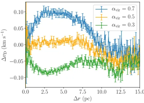
Fig.5showsvM(r), and Fig.6vD(r) for all three Plummer spheres. In both figures, the green lines are used for theαvir=0.3 Plummer sphere, orange for theαvir =0.5 Plummer sphere, and blue for theαvir=0.7 Plummer sphere.

In Fig.5all three lines have the same shape: largevMat low rwhich decreases towards highr. The reason for this is that Plummer spheres have a high central velocity dispersion (at the deepest part of the potential) which decreases at larger radii. The majority of pairs of stars with lowrare located in the core as, by definition, this area is dense and so contains many stars that are close together. These lowrpairs are therefore made up of stars with a high velocity dispersion so any two star’s velocity vectors are likely to be very different, and the magnitude of this difference, vM, will be large. In contrast, stars that make up highrpairs are predominantly located in the halo, where the velocity dispersion is smaller, sovMis low.

Figure 5. Plot showingvM(r) for three Plummer spheres. Thex-axis

is the physical separationrand they-axis is the velocity differencevM.

vM(r) of theαvir =0.7 case is shown by a blue line, theαvir =0.5 case

by an orange line, and theαvir =0.3 case by a green line.

Figure 6. Plot showingvD(r) for three Plummer spheres. Thex-axis

is the physical separationrand they-axis is the velocity differencevD.

vD(r) of theαvir =0.7 case is shown by a blue line, theαvir =0.5 case

by an orange line, and theαvir =0.3 case by a green line.

There is a clear vertical offset between Plummer spheres with higher virial ratios in this figure. This is because, as virial ratio is the ratio of kinetic to potential energies, stars in regions with high virial ratios will have higher speeds on average. Therefore, velocity differences between pairs of stars in those regions are more likely to be high.

Otherwise, the velocity structures of the three Plummer spheres are near-identical according to vM. There is a ‘kink’ present in all three lines atr _∼11 parsecs. This is just a peculiar feature of this particular Plummer sphere realization (a similar feature is not present in Plummer spheres generated with different random number seeds).

In Fig.6,we showv(r) for each of the Plummer spheres using the directional definitionvD. While in Fig.5all three Plummer spheres showed the same velocity structure with only a vertical offset due to their virial ratio, here the three Plummer spheres appear quite different.

Recall that positivevDis indicative of expansion, and a negative value is indicative of collapse. The blue line (αvir=0.7) has values

D

o

w

n

lo

a

d

e

d

fro

m

h

ttp

s:

//a

ca

d

e

mi

c.

o

u

p

.co

m/

mn

ra

s/

a

rt

icl

e

-a

b

st

ra

ct

/4

8

3

/3

/3

8

9

4

/5

2

5

1

8

4

2

b

y

U

n

ive

rsi

ty

o

f S

h

e

ffi

e

ld

u

se

r

o

n

1

7

Ja

n

u

a

ry

2

0

1

Figure 7. Plot showingvD(r) for theαvir=0.7 Plummer sphere. The

true velocity structure is shown in blue. After the velocities are randomly shuffled between stars, the recalulated velocity structure is plotted in grey. Thex-axis is the physical separation rand the y-axis is the velocity differencevD.

that are generally positive, the orange line (αvir=0.5) is roughly flat, and the green line (αvir=0.3) is always negative.

We examine theαvir =0.5 Plummer sphere (orange line) first. For separations of less than 10 parsecs (i.e. separations that contain the majority of the pairs of stars),vDis flat, showing that stars are equally likely to be moving towards each other as away from each other. This is as would be expected for a region that is in neither bulk expansion nor contraction. At separations above 10 parsecs, the stars are generally moving towards each other. This may be due to stars with such extreme separations being mainly found in the extreme halo of the Plummer sphere, and they are being attracted back towards the centre. As a result, they are moving towards each other on average. However, given the size of the error bars, it is also possible the apparent inconsistency of the velocity structure with zero at large separations is an artefact of stochasticity.

For the collapsing (αvir =0.3) case, the line is below zero at every separation. That means, at every separation, on average, the stars are moving closer together.

The expanding case has positive vD at separations below

∼10 parsecs; on average, stars at these separation are moving away from each other. As in theαvir =0.5 case, stars with extreme sep-arations are found to be moving towards one another. Again, this may be due to stars on the outskirts being attracted back towards the centre or it may due to a combination of stochasticity and large error bars at highr.

Uncertainty over whether a feature is real or an ‘artefact’ can be an issue in bins wherenpairs is low, as is typically the case in largerbins. To examine whether this feature is significant, velocities are shuffled randomly between stars which removes any real velocity structure from the data. The method is then reapplied and any ‘features’ observed in the result must be due to stochasticity. This is done 10 times and the results are plotted in grey in Fig.7. The actual velocity structure is again plotted in blue for comparison. From Fig.7, it is is clear that any ‘features’ in the actual velocity stucture of theαvir=0.7 Plummer sphere atr>∼9 parsecs are not significant. The same analysis is applied to theαvir=0.3 and αvir=0.5 Plummer spheres. In theαvir=0.3 case, all features are found to be significant up tor_∼13 parsecs, and in theαvir=0.5 case, the structure is found to be consistent with the randomized cases (so no systematic expansion or contraction) at allrs.

Figure 8. A distribution with low substructure generated by the box fractal method projected into a 1.8 parsec_×1.8 parsec box. Each star is represented by an arrow. The position of the arrow corresponds to the position of the star and the arrow itself indicates the star’s velocity.

3.1 Interpreting observations

If an observer observed the three spherical clusters in this section, they would find them to be very similar in their spatial structure. An analysis of their velocity magnitudesvMwould show a structure such as in Fig.5and it would be possible to say that they each have a Plummer-like velocity distribution. Additionally, an analysis ofvD(r) would show that one is expanding, another collapsing, and the other appears static.

4 C O M P L E X S U B S T R U C T U R E D R E G I O N S

Plummer spheres are fairly simple example distributions. We now apply the method to complex substructured distributions generated by the box fractal method.

A full description of the box fractal method is available in Good-win & Whitworth (2004); however, a brief overview is given here. A single ‘parent’ star is placed in the centre of a box, and then the box is divided into smaller boxes. The probability that each of these smaller boxes has of containing a ‘child’ star is chosen by the user. If the probability is low the fractal will have a high degree of substructure, and if the probability is large the fractal will be more smooth. If a box does contain a child star, it is placed approximately in the centre of the box (noise is added to the position to avoid an obviously gridlike structure). The velocity of the child star is the same as its parent’s velocity plus some random component. After this, each child star becomes a parent and the process is repeated to produce the desired number of stars (extra stars can be deleted at random).

Note that here we are only interested in investigating the appli-cation of the VSAT method to substructured distributions, so the absolute values of e.g. radius and virial ratio are unimportant.

4.1 Distributions with low substructure

An example of a fractal with low substructure and 1000 stars is shown in Fig. 8and the arrows show 2D velocity vectors. Clear

//a

ca

d

e

mi

c.

o

u

p

.co

m/

mn

ra

s/

a

rt

icl

e

-a

b

st

ra

ct

/4

8

3

/3

/3

8

9

4

/5

2

5

1

8

4

2

b

y

U

n

ive

rsi

ty

o

f S

h

e

ffi

e

ld

u

se

r

o

n

1

7

Ja

n

u

a

ry

2

0

1

Figure 9. The velocity structure of the distribution with low substructure shown in Fig.8. The velocity structurevM(r) is shown by a blue line

andvD(r) by an orange line.

structure in both the positions and velocities of the stars is obvious, but too complex to interpret by eye in any meaningful way. It is pos-sible to tell there is substructure, but without other information the eye could not reasonably judge the degree of velocity substructure or how it is distributed.

In Fig.9,we show the magnitude (blue line) and directional (or-ange line)v(r) plots for the fractal in Fig.8(note that everything is done in 2D).

vM(r) (blue line), is ∼2 km s−1 when the separations are low, rising to_∼3 km s−1_{at separations of}

∼0.7 parsecs and then remaining roughly constant.

This initial increase ofvM withris because, as described above, when child stars are produced they inherit most of their ve-locities from their parents, plus a random component. As a result, in the completed distributions, the stars closest together have very sim-ilar velocity vectors, so the magnitude of their difference,vM, is small. Stars further away from each other are very distantly ‘related’ so have very different velocity vectors and theirvMis big.

The 0.7 parsecs length scale is significant because it is the ap-proximate radius of the distribution. Stars separated by this length scale or greater are generated from different ‘child stars’ of the very first generation in the production of the fractal. The random changes applied at each generation after that average to a net ad-ditional difference of zero, sovM remains roughly flat atr≥ 0.7 parsecs.

The directional velocity structure,vD(r) (orange line), is al-ways positive meaning that stars tend to move away from each other on all scales. There is some structure invDshowing that expan-sion increases on scales up to 0.5 parsecs, then is roughly even, before increasing again on scales of>1 parsec.

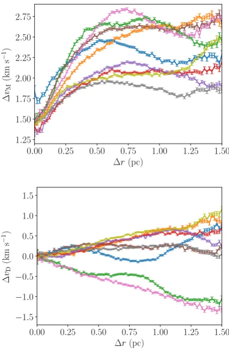
Fig.10showsvM(r) (top panel) andvD(r) (bottom panel) for nine distributions statistically identical to that in Fig.8(only the random number seed used to generate the distributions has been changed). Each distribution has the same colour in both panels.

In the top panel of Fig.10, every distribution’s velocity magnitude structure has the same basic shape: lowvMat small separations which increases with separation to up to around 0.7 parsecs and then is roughly flat. That said, the details of each individual line (distri-bution) are different, and some show ‘structure’ at larger scales.

In the bottom panel of Fig.10,some distributions have predomi-nantly negative (collapsing)vDand some predominantly positive

Figure 10. This figure showsvM(r) (top panel) andvD(r) (bottom

panel) of nine distributions with low substructure generated by the box fractal method.

(expanding) because the box fractal method does not preferentially make either expanding or collapsing distributions. There are fea-tures visible on individual lines in this plot, reflecting that individual distributions (and parts of individual distributions) do have some ve-locity structure.

4.2 Highly substructured distributions

We now examine in detail a distribution with high substructure, illustrated in Fig.11, again with arrows showing the 2D velocities. This distribution has very clear spatial and velocity structure on a variety of scales. Highly substructured distributions are produced using the box fractal method by reducing the probability of each box containing a ‘child’ star. The resulting distribution is less smooth as stars only continue to be generated in boxes that do have children.

The velocity structure of the highly substructured distribution from Fig.11is shown in Fig.12, wherevM(r) is shown by the blue line andvD(r) is shown in orange.

Broadly, thevM(r) of the highly substructured distribution has the same shape asvM(r) of the distribution with low sub-structure:vMincreases withrand then plateaus. However, as we would expect, in the highly substructured case, the line has ad-ditional features, including a plateau at_∼0.3 parsecs and a dip at r>1.1 parsecs. As will be shown in Fig.14and discussed later,

D

o

w

n

lo

a

d

e

d

fro

m

h

ttp

s:

//a

ca

d

e

mi

c.

o

u

p

.co

m/

mn

ra

s/

a

rt

icl

e

-a

b

st

ra

ct

/4

8

3

/3

/3

8

9

4

/5

2

5

1

8

4

2

b

y

U

n

ive

rsi

ty

o

f S

h

e

ffi

e

ld

u

se

r

o

n

1

7

Ja

n

u

a

ry

2

0

1

Figure 11. A highly substructured distribution generated by the box fractal method projected into a 1.8 parsec_×1.8 parsec box. Each star is represented by an arrow. The position of the arrow corresponds to the position of the star and the arrow itself indicates the star’s velocity.

Figure 12. The velocity structure of the distribution with high substructure shown in Fig.11. The velocity structurevM(r) is shown by a blue line

andvD(r) by an orange line.

the features inv(r) due to the velocity substructure are often significant in the highly substructured distributions.

ThevD(r) of the distribution in Fig.11will now be examined in detail in order to demonstrate using the velocity structure plots to investigate the detailed dynamical structure of a region (recall that this is the orange line in Fig.12). Inspection of this figure shows a ‘peak’ invDbetweenr∼0.3 andr∼0.6 parsecs and a ‘trough’ invDbetweenr∼0.8 andr∼1.2 parsecs.

To interpret these features, we can consider which stars contribute more than others in these separation ranges. For example, if a star is in densely populated area, it would be part of many lowr pairs and would appear many times in lowrbins. Understanding which stars are contributing most heavily to the interesting regions of the velocity structure (in this example’s case 0.3–0.6 parsecs and 0.8–1.2 parsecs) helps us to understand the structure. Accordingly,

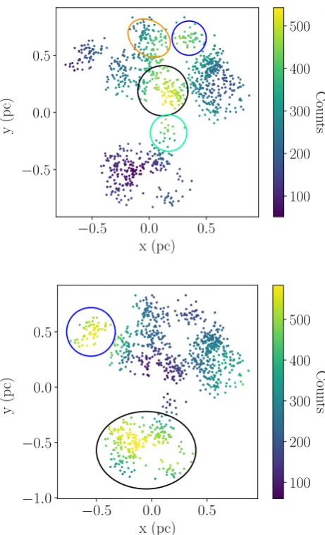
Figure 13. This figure shows the highly sustructured distribution from Fig.11. The stars are colour-coded according to how many times they appear inrbins between 0.3 and 0.6 parsecs (top panel), and between 0.8 and 1.2 parsecs (bottom panel).

the number of times each star appears inrbins between 0.3 and 0.6 parsecs is counted. The fractal is plotted with the stars colour-coded by their counts in these bins in the top panel of Fig.13. The same is done for therbins between 0.8 and 1.2 parsecs in the bottom panel of Fig.13.

First, we will look at the simpler case, which for this distribution is ther0.8–1.2 parsecs range, wherevDis negative. Inspection of the bottom panel of Fig.13shows that two clumps contribute strongly to these bins. These clumps have been circled in blue and black on the figure for clarity. Comparison of this figure with Fig.11 shows that these clumps are moving towards each other, thereforevD is negative in this r range. From this analysis, we can anticipate that these clumps will continue to move towards one another (at least in the short term, and in the 2D plane we are observing – we have no idea here about the third dimension of either position or velocity).

The 0.3–0.6 parsecs range is more complicated. Inspection of the top panel of Fig.13shows that stars in a small clump at coordi-nates around (0.15, 0.15) parsecs which has been circled in black contribute most often to these bins. The stars in several surrounding

//a

ca

d

e

mi

c.

o

u

p

.co

m/

mn

ra

s/

a

rt

icl

e

-a

b

st

ra

ct

/4

8

3

/3

/3

8

9

4

/5

2

5

1

8

4

2

b

y

U

n

ive

rsi

ty

o

f S

h

e

ffi

e

ld

u

se

r

o

n

1

7

Ja

n

u

a

ry

2

0

1

which is moving to the north-west, and the other one circled in blue moving east. Therefore, these three clumps are all moving away from each other, resulting invDbeing positive. In particular, the clump circled in orange is moving directly away from the main body of the distribution. In the short term, we would expect this clump to continue to separate from the majority of the distribution (at least in this projection).

There is one other clump with stars which contribute significantly to the 0.3–0.6 parsecsrbins, which is in the south and circled in green. This clump is moving northeast, directly towards the central clump and the clump circled in blue (so negativevD) and away from the clump circled in orange (positivevD). Although thevD contribution from stars in this clump is mostly negative, the number of stars it contains is small, so it is easy to explain why the mean vDin the 0.3-0.6 parsecsrrange is positive. It seems likely that the black- and green-circled clumps will continue to move towards each other in the short term.

In summary, with only the raw stellar positions and velocities shown in Fig.11,the complex velocity structure of the distribution is very difficult to understand or make judgements on by eye. The method presented in this paper has been used to explore and interpret the dynamical state of this distribution and make predictions about its short-term future.

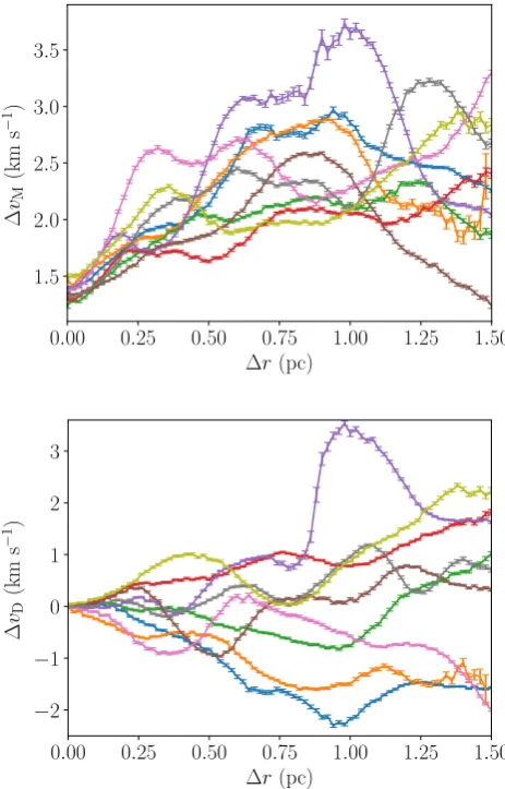
For the purpose of comparison, nine additional highly substruc-tured regions are generated using the same method but different random number seeds. These region’s velocity structures are shown in Fig.14where the top panel showsvM(r) and the bottom panel

vD(r).

The first feature of note is that there is much less structure in both panels of Fig.10than in their corresponding panels in Fig.14, which reflects the significant velocity substructure in this latter set of distributions. This is useful because while it is easy to distinguish the differing levels of spatial structure in Figs8and 11 by eye the distributions are too complex to tell simply by looking if the velocity structures are different. Therefore, even if the actual degree of velocity structure in each set of distributions were unknown, we could still say with confidence that there is significantly more velocity structure in this latter set.

We also note that in Fig.14each individual line in both panels appears quite different from the others. This is unsurprising as the distributions are produced using different random number seeds so each is unique, and the distributions are highly substructured so two statistically identical distributions may have very different forms .1 In the top panel (vM), the velocity structures show a general upwards trend; although individual structures show significant de-viation from this (as was mentioned in the discussion of Fig.12) on the wholevMcorrelates positivity withr. This increase of vMwithris a result of the box fractal generation method which produces distributions where stars that are near one another have similar velocities and stars that are far apart have very different ve-locities. The magnitude of the features on each line makes it difficult to say with confidence if there is a plateau at larger.

1_{This raises the question as to if these distributions are indeed ‘the same’,}

however, that is a discussion beyond the scope of this paper.

Figure 14. This figure shows the velocity structurevM(r) (top panel)

andvD(r) (bottom panel) of nine highly substructured distributions

gen-erated by the box fractal method.

In the bottom panel, as is the case in Fig.10, some distributions have predominantly negativevDand some predominantly positive vDas the box fractal method is not biased towards making either expanding or collapsing distributions.

5 I N C L U D I N G O B S E RVAT I O N A L U N C E RTA I N T I E S

In this section, we test whether the method is robust when faced with imperfect data.

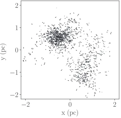
The velocity structure of a simulated star cluster is measured, then observational errors are applied to the data, and the velocity struc-ture is re-calculated. The ‘true’ velocity strucstruc-ture and ‘observed’ velocity structure are then compared. A simulation with an unusual spatial and velocity evolution is used to make this more challenging. The cluster is taken from Arnold et al. (2017). That paper gives all the details of the simulations, but this cluster containsN₌1000 stars with masses drawn from the Maschberger IMF (Maschberger 2013) using a lower limit of 0.1M_⊙and an upper limit of 50M_⊙. It has been evolved for 2 Myr and has split into a binary cluster as shown in Fig.15.

Although the results presented here concern only this cluster, the same procedure has been applied to a variety of other simulated clusters, and similar results are found.

D

o

w

n

lo

a

d

e

d

fro

m

h

ttp

s:

//a

ca

d

e

mi

c.

o

u

p

.co

m/

mn

ra

s/

a

rt

icl

e

-a

b

st

ra

ct

/4

8

3

/3

/3

8

9

4

/5

2

5

1

8

4

2

b

y

U

n

ive

rsi

ty

o

f S

h

e

ffi

e

ld

u

se

r

o

n

1

7

Ja

n

u

a

ry

2

0

1

Figure 15. A cluster from a simulation with an unusual velocity evolution. Observational errors are applied to this cluster and the ‘true’ and ‘observed’ velocity structures are compared.

5.1 Velocity uncertainties

As stated in Section 2, this paper only considers errors on velocities as they are typically significantly larger than errors on positions. We also assume that all stars in the analysis are true members of the cluster. Later, we remove low-mass stars and examine the impact on the results, but do not add ‘contaminants’ (how important these are will vary significantly depending on the observational data set). Observational uncertainties are simulated by replacing each star’s ‘true’ velocity with an ‘observed’ velocity with an associated error. The observed velocity is drawn from a Gaussian centred on the true velocity. The width of the Gaussian used is the observational uncertainty being simulated,σsim(i.e. the true velocity usually lies within the error bar of the observed velocity). This is done for thex,y, andzcomponents of the velocity separately, i.e. the true xvelocity of a star is replaced with an observedxvelocity, etc. Here, σsim values of 0, 0.4, 0.8, 1.2, and 1.6 km s−1 are used. Theσsim = 0 km s−1case is the true velocity structure as there is no observational uncertainty (although it still has an uncertainty associated with stochasticity as in all previous cases).

For eachσsim, the observedvM(r) andvD(r) are calcu-lated. These are shown in Fig.16where the velocity structure with σsim =0 km s−1is shown by the blue line, 0.4 km s−1is the orange line, 0.8 km s−1_{is the green line, 1.2 km s−}1 _{is the red line, and} 1.6 km s−1_{is the purple line.}

From inspection of the top panel, it is clear that the meanvM, vM, that is found increases with observational uncertainty from

∼2 km s−1 _{when there is no observational error, o}

∼2.2 km s−1 when the error isσsim = 0.4 km s−1, and asσsim increases this trend continues.2 _{The reason for this is that uncertainties in the} velocities cause the velocity dispersion to be artificially inflated. As a result, the observed difference between any two velocity vectors is more likely to be larger rather than smaller than the ‘true’ difference.

2_{Note that this increase is not equal toσ}

sim√2 as may be expected.

structure less well, but the overall structure remains essentially recognisable even in the cases where the simulated uncertainty on each velocity component is greater than the 3D velocity dispersion of the cluster (1.53 km s−1_{). From this, we conclude that the method} deals well with observational uncertainty up to and potentially be-yond the point where the errors are as large as the velocity dispersion of the region. ForGaia,velocity uncertainties depend largely on the apparent magnitude of the source. Table B.1 in Lindegren et al. (2018) gives median values of these uncertainties as a function of apparent magnitude for Gaia DR2. For a G-dwarf at_∼1 kpc, we would expect errors in proper motion of around 0.3–1 km s−1_.4

In the bottom panel of Fig.16,we show the directional velocity structurevD(r) (with the lines for different errors having the same colours as in the top panel). What is obvious here is that the observational errors have essentially no effect on the directional structure. This is because even with uncertainties the apparent di-rections of motion are usually roughly correct, and errors between pairs tend to average out rather than sum (as they did above). (Note that we assume the errors are uniform across our ‘field of view’, if they are not this could introduce a bias but we have not investigated this potential effect.)

5.2 Mass cutoffs

A probable bias in observations is to not observe low-mass stars as they are typically faint. (Note here that larger errors on fainter star’s velocities would be included in the error propagation). We examine the effect of selection limits by removing stars of increasingly high mass from our region.

The region has 1000 stars in total which reduces to 428 stars of >0.3M_⊙, 207 stars of>0.6M_⊙, 128 stars of>0.9M_⊙, and only 83 stars of>1.2M_⊙(these mass limits are rather arbitrary and are just chosen as examples).

Fig.18shows the differentvM(r) (top panel), andvD(r) (bottom panel) plots. Different coloured lines represent different mass limits as described in the figure.

From Fig.18, we see that the same basic velocity structure is observed at all mass limits for bothvM(r) andvD(r). There does appear to be a sytematic increase in the amplitude of both vM(r) andvD(r) at highr and high mass cutoff. This

3_{The Monte Carlo method works well, but not perfectly. Overlaying the}

lines exactly allows their features to be compared more easily by eye.

4_{The random error in DR2 for G magnitudes of 15–17 is}

∼0.06–0.2 mas yr−1, however there is also a systematic error at the close angular separations we are interested in of∼0.1 mas yr−1(see Lindegren et al. (2018) for details).

//a

ca

d

e

mi

c.

o

u

p

.co

m/

mn

ra

s/

a

rt

icl

e

-a

b

st

ra

ct

/4

8

3

/3

/3

8

9

4

/5

2

5

1

8

4

2

b

y

U

n

ive

rsi

ty

o

f S

h

e

ffi

e

ld

u

se

r

o

n

1

7

Ja

n

u

a

ry

2

0

1

Figure 16. The velocity structure of the cluster in Fig.15with simulated observational uncertainties applied. The top panel showsvM(r) and the bottom

panel showsvD(r). In both panels, a blue line is used for the true velocity structure, orange for a simulated observational uncertainty of 0.4 km s−1, green

for 0.8 km s−1_{, red for 1.2 km s}−1_{, and purple for 1.6 km s}−1_.

Figure 17. Top panel of Fig.16with each line shifted such that theirvMmatches that of the true velocity structure.

D

o

w

n

lo

a

d

e

d

fro

m

h

ttp

s:

//a

ca

d

e

mi

c.

o

u

p

.co

m/

mn

ra

s/

a

rt

icl

e

-a

b

st

ra

ct

/4

8

3

/3

/3

8

9

4

/5

2

5

1

8

4

2

b

y

U

n

ive

rsi

ty

o

f S

h

e

ffi

e

ld

u

se

r

o

n

1

7

Ja

n

u

a

ry

2

0

1

Figure 18. The velocity structure of the cluster in Fig.15as measured by the method using different mass cutoffs. The top panel showsvM(r) and the

bottom panel showsvD(r). In both panels, the blue line is the result using all stars, the orange line using stars above 0.3M_⊙, green uses those above 0.6 M_⊙, red above 0.9M_⊙, and purple above 1.2M_⊙.

apparent increase is not observed in other simulations from the same set. It is therefore determined to be a peculiarity of this particular simulation like the apparent ‘kink’ observed in Fig.5.

The overall robustness of the measured velocity structure against mass cutoffs is encouraging, especially considering the 1.2M_⊙ cutoff leaves only 83 of the cluster’s original 1000 stars remaining, but it is still able to reproduce the shape of the true underlying velocity structure reasonably well.

That each of our lines for different mass limits are very similar shows that in this simulation they all trace a similar velocity ‘field’. This may not be the case in reality, for example in some regions the star’s spacial and velocity distributions may be a functions of mass (mass segregated regions being an obvious example).

Nevertheless, we can only measure the velocity structure of the stars which are detected, and from these tests this appears to be robust.

As the mass of the cut-off increases, the level of noise increases which is unsurprising as fewer stars survive the higher the cutoff.

When there are large error bars as a result of low-N,the random-ization approach used in Section 3 could be used to confirm which features in the observed structure are significant.

6 M U LT I P L E S T E L L A R S Y S T E M S

So far, we have assumed all stars are single. However, in obser-vational data and more realistic simulations, many stars will be in binaries or higher-order multiples. Multiple systems, particularly those in close orbits, often have high orbital velocities. However, from the point of view of the global velocity structure of a region, a system’s centre of mass velocity better describes the motion of the stars over time than their individual velocities. Here, the impact of binary systems on the velocity structure returned by the method is examined (higher order multiples are not included for the sake of simplicity).

This is done by first generating a distribution of 5000 artificial binary systems. This large number is chosen to dampen noise due

//a

ca

d

e

mi

c.

o

u

p

.co

m/

mn

ra

s/

a

rt

icl

e

-a

b

st

ra

ct

/4

8

3

/3

/3

8

9

4

/5

2

5

1

8

4

2

b

y

U

n

ive

rsi

ty

o

f S

h

e

ffi

e

ld

u

se

r

o

n

1

7

Ja

n

u

a

ry

2

0

1

tribution between 0.2 and 1 (Raghavan et al.2010) and the mass of the primary is multiplied by this factor to produce the mass of the secondary. The period,Pof the system is drawn from a lognormal distribution centred on logP ₌5.03 with a standard deviation of 2.28 (herePis in days (d)) (Raghavan et al.2010). From this, the semimajor axis of the system is calculated. Orbits are circular and the phase and inclination angle of the system are chosen randomly. The position and velocity of the system’s centre of mass are also drawn randomly, the position from a uniform distribution within a 1 parsec_×1 parsec_×1 parsec cube, and the velocity from a Gaus-sian distribution with a standard deviation of 3 km s−1_{in a random} direction.

Synthetic proper motion and radial velocity measurements are then generated from this distribution. Proper motion measurements are produced by evolving the distribution forwards by 5 years (grav-itational forces exerted on the systems by each other are neglected because of the shortness of this time-scale). The change in each star’s position in thex₋yplane is used to calculate its observed proper motion. Stars’s radial velocities are taken to be their instan-taneous velocities in thez-direction.

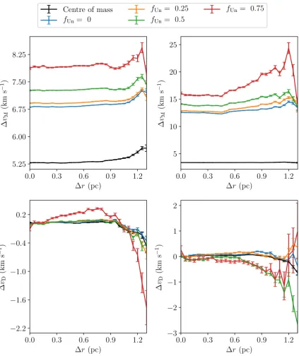
In Fig.19,we show the velocity structure of this distribution of binaries. In the left column, are the results using proper motion (2D) velocities, and in the right column are results using radial (1D) velocities velocities. The top row usesvMfor each case, and the bottom row usesvD.

In all four panels, the results using the system centre of mass ve-locities are shown by black lines. The centre of mass veve-locities more accurately describe the distribution’s underlying velocity structure than the velocities of the individual stars which contain an orbital component. All four of these black lines are generally flat as ex-pected for a random velocity field. There is a slight deviation from this at largerbecause asrincreases fewer and fewer systems in the 1 parsec square box are sufficiently far apart to populate these bins, making them vulnerable to stochasticity (see earlier).

The other coloured lines in Fig.19are the velocity structure recal-culated using the individual velocities of (some) stars. To model ob-servational limitations, we remove some fraction,fUn, of the lowest-mass (hence lowest luminosity) stars. ForfUn =0 (blue lines), all primaries and companions are observed. For an unobserved frac-tionfUn =0.25 (orange lines), the 25 per cent lowest-mass stars are ‘unobserved’ and are not included in the velocity structure cal-culation, and similarly forfUn=0.5 (green lines), andfUn=0.75 (red lines).

Note that (as described earlier) as the size of the region is 1 parsec-by-1 parsec any features on scales greater than 1 parsec should be ignored (or at least taken with extreme caution).

We also note that the results described here reflect the impact of binary stars in the worst case scenario: the binary fraction is 100 per cent, and only a single epoch of radial velocity data is used. Nine other distributions, each with 5000 binary systems, are produced and analysed as described here. Their results show the same general trends as the one presented in this paper.

We will first discuss the results usingvM(top row of Fig.19). In both the cases, where the proper motions (left-hand panel) and the radial velocities (right-hand panel) are used, the flat shape of the centre of mass determination of vM(r) (the black lines)

case, this artificial structure predominantly increasesvM. In the nine other realizations of the distribution, however, there is an even spread between cases where the artificial structure increases and decreasesvM.

It is clear from the figure that the results using stellar velocities are off-set to highervM. This is due to an inflation of the ‘velocity dispersion’ from the extra velocity components from binary motion. The degree of the inflation is larger in the radial velocity case than the proper motion case as orbital motions, particularly in tight binaries, can add significant instantaneous component to the stellar velocity but these are somewhat ‘washed out’ by the time baseline of proper motion observations. As discussed in Section 5.1, the inflation ofvMhas minimal impact on the interpretation of the distribution’s velocity structure. Overall, the agreement between the velocity structure of the region as calculated using the centre of mass velocities, and the structure using the stellar velocities is good for all but the highestfUnandr.

The bottom row of Fig.19showsvD(r) using proper motions (left-hand panel) and radial velocities (right-hand panel). In both cases the directional velocity structure is extremely similar for the centres of mass (black lines), and complete or fairly complete binary samples (blue and orange lines): a flat distribution at zerovD. When half, or more, of low-mass stars are unobserved (fUn =0.5 green line,fUn=0.75 red line), some artificial structure appears. For mostrs, this structure has an amplitude below 0.3 km s−1_{, so} would almost certainly be lost in the noise of real data. As in the vM results, the artificial structure can both increase or decrease vD, and is most severe at highr.

For the case presented in Fig.19, thefUn=0.5 results using the proper motions (left panel, green line) is startlingly well behaved. This is a quirk of the binary distribution presented here; in general, there is some artificial structure in thefUn=0.5 results. In the radial velocity results, there is more deviation, which is more typical.

It is worth reiterating that in the case of radial velocities a single epoch of observations is assumed. If there were multiple epochs, an observer could potentially estimate binary system’s centre of mass velocity, even if only one star is observed. If an orbital solution cannot be found but a fluctuation in a star’s radial velocity is ob-served, the suspected binary could be removed from the data set. This prevents contamination of the calculated velocity structure by an unknown orbital component and, as was shown in Section 5.2, the method is robust even when a high fraction of stars are not observed.

As described, there are 10 000 stars in the distribution used to produce Fig. 19 and this largeN is chosen to dampen noise due to the stochasticity in the distribution (except, as discussed, at highrwherenpairsunavoidably becomes low). However, many observational data sets have much lower N. For comparison, the procedure described above is repeated for a distribution of 1000 stars (500 binary systems). The results are shown in Fig.20.

The velocity structure as calculated using the system’s centres of mass velocities is less flat than in Fig. 19due to the increase in stochasticity caused by lowerN. The velocity structure of the systems themselves is not of interest here however; it is the degree of agreement between it and the velocity structure calculated using the stellar velocities that is being examined.

D

o

w

n

lo

a

d

e

d

fro

m

h

ttp

s:

//a

ca

d

e

mi

c.

o

u

p

.co

m/

mn

ra

s/

a

rt

icl

e

-a

b

st

ra

ct

/4

8

3

/3

/3

8

9

4

/5

2

5

1

8

4

2

b

y

U

n

ive

rsi

ty

o

f S

h

e

ffi

e

ld

u

se

r

o

n

1

7

Ja

n

u

a

ry

2

0

1

Figure 19. The velocity structure of a distribution of 5000 binary systems. The top two panels use thevMdefinition and the bottom twovD. The left-hand

column calculates the velocity structure using synthetic proper motion data, and the right hand one synthetic radial velocity data. In all four panels, the black lines are the velocity structure calculated using the centre of mass velocities of the binary systems. The other lines use the velocities of the individual stars. The blue lines are the velocity structure calculated when all stars in the sample are observed (the unobserved fractionfUnis zero). The orange lines are the results

whenfUnis 0.25, the green whenfUnis 0.5, and the red whenfUnis 0.75.

Inspection of Fig. 20 shows the results are noisier and have larger uncertainties than those in Fig.19which can be attributed to the lower N. Nevertheless, the agreement is relatively good between the results using centre of mass velocities and stel-lar velocities although, as was the case in Fig. 19, this be-comes worse at high r and fUn, and there is an increase in vMwithfUn. Again, nine other distributions of 500 binary sys-tems were generated and show the same general trends as in Fig.20.

We now summarize the effect of binaries. Binaries ‘inflate’vM with respect to the binary centre of mass determination (exactly by how much depends on the binary population); however, the overall structure ofvMremains similar even when a significant fraction of low-mass stars are unobserved. The level and structure ofvDremains very similar, though there are deviations when the ‘unobservable’ fraction is very high.

What is recomforting is that the VSAT method is capable of extracting real structure from even a single epoch of radial velocity

//a

ca

d

e

mi

c.

o

u

p

.co

m/

mn

ra

s/

a

rt

icl

e

-a

b

st

ra

ct

/4

8

3

/3

/3

8

9

4

/5

2

5

1

8

4

2

b

y

U

n

ive

rsi

ty

o

f S

h

e

ffi

e

ld

u

se

r

o

n

1

7

Ja

n

u

a

ry

2

0

1

Figure 20. This figure has the same structure as Fig.19but it shows the velocity structure of a distribution of 500 binary systems rather than 5000. The top panels use thevMdefinition and the bottom panelsvD. The left column calculates the velocity structure using proper motions, and the right-hand one uses

radial velocities. The black lines show the velocity structure calculated using the binary system’s centre of mass velocities, and the other lines are the velocity structure as calculated using the velocities of the individual stars. The blue lines use all stars in the sample, the orange lines are the results whenfUnis 0.25,

the green whenfUnis 0.5, and the red whenfUnis 0.75.

data contaminated with binary motions. Such an analysis should be treated with rather more caution than proper motion data or multi-epoch radial velocity data, but it still contains useful information.

7 C O N C L U S I O N S

In this paper, we present a method of examining the velocity struc-ture of star-forming regions by plotting the physical separation of pairs of stars (r) against their mean velocity difference (v).

Distributions ofv(r) for different regions can be directly com-pared to each other. Two definitions ofvare used, the ’magnitude’ definition (vM), and the ‘directional’ definition (vD).

This method does not require the region’s centre or radius to be defined, requires no assumptions about the region’s morphology, and can be applied to data in any number of dimensions in any frame of reference. The method also includes the treatment of ob-servational errors, and is shown to be useful even for data with large errors.

D

o

w

n

lo

a

d

e

d

fro

m

h

ttp

s:

//a

ca

d

e

mi

c.

o

u

p

.co

m/

mn

ra

s/

a

rt

icl

e

-a

b

st

ra

ct

/4

8

3

/3

/3

8

9

4

/5

2

5

1

8

4

2

b

y

U

n

ive

rsi

ty

o

f S

h

e

ffi

e

ld

u

se

r

o

n

1

7

Ja

n

u

a

ry

2

0

1

AC K N OW L E D G E M E N T S

BA acknowledges PhD funding from the University of Sheffield. Thanks also to Murali Haran for useful correspondence and to Liam Grimmett and Gemma Rate for useful discussions.

R E F E R E N C E S

Aarseth S. J., Henon M., Wielen R., 1974, A&A, 37, 183 Alfaro E. J., Gonz´alez M., 2016,MNRAS, 456, 2900

Allison R. J., Goodwin S. P., Parker R. J., Portegies Zwart S. F., de Grijs R., Kouwenhoven M. B. N., 2009,MNRAS, 395, 1449

Arnold B., Goodwin S. P., Griffiths D. W., Parker R. J., 2017,MNRAS, 471, 2498

Cartwright A., Whitworth A. P., 2004,MNRAS, 348, 589 Da Rio N. et al., 2017,ApJ, 845, 105

Franciosini E., Sacco G. G., Jeffries R. D., Damiani F., Roccatagliata V., Fedele D., Randich S., 2018,A&A, 616, L12

Gagn´e J., Faherty J. K., 2018,ApJ, 862, 138

Galli P. A. B., Bertout C., Teixeira R., Ducourant C., 2013,A&A, 558, A77 Goodwin S. P., Whitworth A. P., 2004,A&A, 413, 929

Kounkel M. et al., 2018,AJ, 156, 84

Krige D. G., 1951, PhD thesis. University of Witwatersrand

Kuhn M. A., Hillenbrand L. A., Sills A., Feigelson E. D., Getman K. V., 2018, preprint (arXiv:1807.02115)

Lindegren L. et al., 2018,A&A, 616, A2 Maschberger T., 2013,MNRAS, 429, 1725

Maschberger T., Clarke C. J., 2011,MNRAS, 416, 541 Matheron G., 1963,Econ. Geol., 58, 1246

Raghavan D. et al., 2010,ApJS, 190, 1

Wright N. J., Mamajek E. E., 2018,MNRAS, 476, 381

Wright N. J., Bouy H., Drew J. E., Sarro L. M., Bertin E., Cuillandre J.-C., Barrado D., 2016,MNRAS, 460, 2593

A P P E N D I X : C O R R E C T I N G I N F L AT I O N

The increase invM with uncertainty will now be explained in more detail. As only the magnitude definition ofvis affected, the Msubscript will be dropped to avoid overly long subscripts in this appendix.

The true velocities of stars in a region (vT) have some distribution. A cartoon, idealized picture of this is shown by a blue line in Fig.A1, where thex-axis is velocity, and they-axis is the probability of a star having a given velocity. Due to observational uncertainties, it is impossible to perfectly measure the true velocitiesvT, and instead we observe velocitiesvobs. The effect of observational uncertainties is to smear out the true velocity distribution. The observed velocity distribution is shown by the orange line in Fig.A1for our cartoon

Figure A1. Cartoon depicting the broadening of the observed velocity distribution due to observational uncertainties. Thex-axis shows a range of velocities and they-axis their probability. A true velocity distribution (in blue) is broadened into the observed velocity distribution (in orange).

case. Notice that the observed velocity distribution is wider that the true velocity distribution.

When the velocity difference between two stars in a region is measured this can be thought of as drawing two velocities from the velocity distribution and calculating the difference between them. If the distribution is narrow, then the range of likely velocities is small so the two velocities drawn will usually have a small difference between them, thereforevwill be small. In contrast, if the distri-bution is wide it is more likely that any two values drawn will be very different, sovwill be large. As discussed, the observed ve-locity distribution is wider than the true veve-locity distribution, so the observed mean velocity difference between pairs of stars (vobs) is larger than the true mean velocity difference between pairs of stars (vT). Because the width of thevobsdistribution increases with uncertainty, so doesvobs. This is why in the top panel of Fig.16 there is a positive correlation betweenvandσsim.

As discussed above, observational errors broaden the observed velocity distribution, so the true velocity distribution can be crudely approximated by a narrower version of the observed velocity dis-tribution. In brief, the observed velocity distribution is narrowed by different amounts and Monte Carlo methods are used to find which width best reproduces the observed velocity distribution once obser-vational errors are applied. Many velocities are then drawn from this best-fitting distribution, andvis calculated. This is the estimated value ofvTgiven the observed velocities and the errors.

The exact method used will now be described in more detail. Diagrams shown in Fig.A2are referred to to aid this description. For both of these plots the x-axis is velocity, and the y-axis is probability. They show how the method would be applied to some cartoon non-Gaussian velocity distribution (the black line in the left-hand panel of Fig.A2).

First a Gaussian kernel is applied to the observed velocities to produce a probability density function (pdf) of the observed veloc-ities (red line in both panels of Fig.A2). It is assumed that the true velocities pdf is the same shape, but narrower. How much narrower is unknown, and though it can be analytically calculated if the dis-tributions are Gaussian that will often not be the case. Instead, many different widths are tested, each model being a ‘guess’ at the true velocity structure. To prevent Fig.A2becoming overcrowded, only three models are shown (blue dashed lines). In this diagram, it is

//a

ca

d

e

mi

c.

o

u

p

.co

m/

mn

ra

s/

a

rt

icl

e

-a

b

st

ra

ct

/4

8

3

/3

/3

8

9

4

/5

2

5

1

8

4

2

b

y

U

n

ive

rsi

ty

o

f S

h

e

ffi

e

ld

u

se

r

o

n

1

7

Ja

n

u

a

ry

2

0

1