Electrolytes at spherical dielectric interfaces

(1)

Electrolytes at spherical dielectric interfaces

R. A. Curtis and L. Luea兲

School of Chemical Engineering and Analytical Science, The University of Manchester, P.O. Box 88, Sackville Street, Manchester M60 1QD, United Kingdom

共Received 22 July 2005; accepted 6 September 2005; published online 31 October 2005兲

A variational theory is developed and applied to study the properties of dielectric spheres immersed in a symmetric electrolyte solution. In the limit that the radius of the sphere becomes much larger than the Debye screening length, the system reduces to that of a planar dielectric interface. For this case, the excess surface tension obtained by the variational theory reduces to the Onsager-Samaras 关J. Chem. Phys. 2, 528共1934兲兴limiting law at low electrolyte concentrations. As the radius of the dielectric sphere decreases, the excess surface tension also decreases. The implications of this work to protein-salt interactions and the salting out of proteins are discussed. ©2005 American Institute of Physics.关DOI:10.1063/1.2102890兴

I. INTRODUCTION

Most biological systems of interest are aqueous electro-lyte solutions containing macromolecules or macromolecular structures共e.g., proteins, polysaccharides, micelles, bilayers, etc.兲. Understanding these systems requires determining the interactions between these colloids and the surrounding aqueous electrolyte solvent and also the solvent-mediated in-teractions between the colloids. The traditional approach to describing the interaction of the electrolyte solution with the colloid is based on the Poisson-Boltzmann equation. How-ever, one of the inadequacies of these approaches is that they predict an excess of salt in the domain of a charged colloid, whereas for most proteins in moderately concentrated salt solutions, salt is preferentially excluded.1 As discussed be-low, one route to correcting this shortcoming is to include the influence of the low dielectric interior of the colloids 共e.g., micelles and proteins兲in the models.

Repulsive image charge forces between ions and a low dielectric boundary result in preferential desorption of salt from the interface. By using a Poisson-Boltzmann approach to quantify the desorption, Wagner2 and Onsager and Samaras3were able to compute the excess surface tension of electrolyte solutions by integrating the Gibbs adsorption equation. Similarly, studies of protein solutions have shown that the exclusion of salt around the protein is correlated with the surface tension increment of the salt indicating that as a first approximation the interior of a protein could be treated as a low dielectric continuum, similar to air.1

The effect of image charges on surface tension and on the force between surfaces is well known for planar geom-etries 共for instance, see Refs. 4–11兲. However, the influence of curvature on these interactions is less well known. Linse12 and Messina13 used Monte Carlo simulations to study the effect of image forces on the electrical double layer about a charged colloid sphere with a different dielectric constant from the surrounding medium. In these studies, the density distribution about the spheres is determined, but the resulting

surface tension was not calculated. Groenewold extended the work of Onsager and Samaras to weakly curved systems14 and found that the surface tension decreased if the surface curved away from the electrolyte solution and increased if it curved toward the solution.

In this work, we examine the excess surface tension of dielectric particles. In particular, we consider a sphere of radius R and dielectric constant ⑀

⬘

that is immersed in a continuous medium of dielectric constant ⑀ containing dis-solved electrolytes. To study this problem, we pursue a field theoretic formulation of the electrolyte problem.15–18 This type of approach has already been applied to a wide range of problems, including electrolytes near planar dielectric interfaces19–21or the potential of mean force between spheri-cal macroions.16,22The advantage of this approach over the traditional Poisson-Boltzmann equation共such as used by On-sager and Samaras and applied by Groenwold to curved di-electric interfaces兲 is that it is able to account for ion-ion correlation effects and the influence of image charge interac-tions can be self-consistently incorporated. In addition, other nonelectrostatic interactions experienced by the ions can be included in the model, such as excluded volume forces11or ion-ion and ion-surface dispersion forces. The latter forces are believed to be important in understanding the specific ion effects, which are significant in moderately concentrated salt solutions.23

The remainder of the paper is organized as follows. In the Sec. II, we present a brief review of the functional inte-gral formulation of electrolyte systems and apply a standard variational approximation to develop the theory. The appli-cation of this theory to bulk electrolyte solutions is given in Sec. III, and its application to an electrolyte at a general dielectric interface is discussed in Sec. IV. The particular examples of planar共where the theory exactly reproduces the Onsager-Samaras limiting law at low electrolyte concentra-tions兲 and spherical interfaces are examined in Sec. V and VI, respectively.

a兲_{Electronic mail: [email protected]}

(2)

II. THEORY

A. Development of the free-energy functional

In this section, we develop a functional integral formu-lation of the grand partition function of an electrolyte solu-tion. This type of formulation has already been presented by previous authors,15–18,24so we only present a brief overview of the main points.

Consider an electrolyte system composed of particles with embedded point charges that are immersed in a continu-ous medium with a spatially varying dielectric constant⑀共r兲

and with a fixed charge distribution ⌺共r兲 imposed on the system共rdenotes the position in the system兲. The chemical potential of particles of type␣is held fixed at␮_␣, and there is a nonuniform external potentialu_␣共r兲acting on each par-ticle. The grand partition functionZGfor this system is given

by25

ZG关␥,⌺兴=

兺

N₁=0

⬁

¯

兺

N_M=0

⬁

兿

␯ 1

N_␯!␭_␯3N␯ ⫻

冕

兿

␶t

dr_␶te−␤E

elec −␤Eref+兺

␣,␬␥␣共r␣,␬兲, 共1兲

where ␤= 1 /共kBT兲, kB is the Boltzmann constant, T is the

absolute temperature,N_␣ is the number of particles of type ␣,r_␣,␬ is the position of the ␬th ion of type ␣,␭␣ is the

thermal wavelength of an ion of type ␣, and ␥_␣共r兲=␤关␮_␣ −u_␣共r兲兴. The interaction energy between the particles is di-vided into an electrostatic contributionEelec_and

nonelectro-static contributionsEref_共_{e.g., due to excluded volume, etc.}_兲_.

The energy of the electrostatic field can be written in terms of the instantaneous charge distributionQ共r兲,26

Eelec=1

2

冕

drdr

⬘

Q共r兲G0共r,r

⬘

兲Q共r

⬘

兲−

兺

_␣_,_␬e␣

se_共_r

␣,␬兲, 共2兲

where G0共r,r

⬘

兲 is the Green’s function associated with the

electrostatics problem, which is defined by the following relation:

− 1

4␲ⵜ ·⑀共r兲ⵜG0共r,r

⬘

兲=␦共r−r

⬘

兲. 共3兲 Physically, the Green’s functionG0共r,r

⬘

兲 is the electric

po-tential at position rthat is generated by a unit point charge located at positionr

⬘

.

The first term on the left side of Eq.共2兲gives the total electrostatic energy, which includes a contribution from the direct interaction of each point charge with itself. This infi-nite self-energy is removed by including the second term on the right side of Eq. 共2兲, which gives the self-energy e_␣se共r兲

=q_␣2G₀free共r,r兲/ 2 of a point charge in an infinite medium with a constant dielectric constant⑀. The Green’s functionG₀freeis given by

G₀free共r,r

⬘

兲= 1 ⑀兩r−r

⬘

兩.

The total charge density is composed of a fixed charge dis-tribution ⌺共r兲 and a contribution from the mobile particles with embedded point charges:

Q共r兲=

兺

␣,␬

q_␣␦共r−r_␣,␬兲+⌺共r兲, 共4兲

whereq_␣is the charge of a particle of type␣.

With this expression for the electrostatic energy, the grand partition function can be rewritten as a functional integral by introducing the Hubbard-Stratonovich transformation27,28to give

ZG关␥,⌺兴=

1

N0

冕

D␺共·兲

⫻exp

再

− 1

2␤

冕

drdr

⬘

␺共r兲G0

−1_共_r_,_r

_⬘

_兲␺共_r

_⬘

_兲

−

冕

dr⌺共r兲i␺共r兲+ lnZGref关␥−qi␺+␤ese兴

冎

,

共5兲

where ZG

ref

is the grand partition function of the reference system 共i.e., the system with no electrostatic interactions兲 and

N0=

冕

D␺共·兲exp

冋

−

1

2␤

冕

drdr

⬘

␺共r兲G0

−1_共_r_,_r

_⬘

_兲␺共_r

_⬘

_兲

册

_.

The function i␺共r兲 can be interpreted as being equal to an instantaneous value of the electrostatic potential, and the functional integral can be thought of as an integral over all possible “shapes” of the electrostatic potential due to the thermal motion of the electrolytes.

B. The variational method

The functional integral representation for the grand po-tential given in Eq.共5兲is exact, although approximate meth-ods are required to solve this equation, such as the mean-field approximation or the loop expansion. In this work, we use a standard variational method,29which has recently been used to study30 electrolyte systems near highly charged ob-jects.

Within the variational method, calculations are per-formed with respect to a reference Hamiltonian, which is typically chosen to be Gaussian. The most general form for a Gaussian Hamiltonian is

−H_K关␺兴= 1

2␤

冕

drdr

⬘

关␺共r兲−␺

¯_共_r_兲兴

⫻G_K−1共r,r

⬘

兲关␺共r

⬘

兲−␺¯共r

⬘

兲兴, 共6兲

where␺¯ is the mean value of the field ␺,

G_K−1共r,r

⬘

兲=G₀−1共r,r

⬘

兲+K共r,r

⬘

兲, 共7兲

and K is an arbitrary screening function. The modified Green’s functionG_K共r,r

⬘

兲represents the electric potential at position r generated by a unit point charge located at posi-tionr

⬘

. It differs from the “bare” Green’s functionG0共r,r

⬘

兲

(3)

Averages taken with respect to the Gaussian Hamil-tonian, given in Eq.共6兲, are denoted by具共¯兲典Kand are

de-fined as

具共¯兲典K⬅

1

NK

冕

D␦␺共·兲共¯兲exp

冋

−

1 2␤

⫻

冕

drdr

⬘

␦␺共r兲G_K−1共r,r

⬘

兲␦␺共r

⬘

兲

册

, 共8兲

where␦␺共r兲=␺共r兲−␺¯共r兲, and the normalization constantN_K is given by

N_K=

冕

D␺共·兲exp

冋

− 1

2␤

冕

drdr

⬘

␺共r兲GK

−1_共_r_,_r

_⬘

_兲␺共_r

_⬘

_兲

册

_.

The grand partition function can then be rewritten in terms of the Gaussian Hamiltonian,

lnZG关␥,⌺兴=

1

2␤

冕

drdr

⬘

i␺

¯_共_r_兲_G 0 −1_共

r,r

⬘

兲i␺¯共r

⬘

兲

−

冕

dr⌺共r兲i␺¯共r兲+ lnNK

N0

+ ln具e−␦HK关␦␺兴典_K_,

共9兲

where the fluctuation Hamiltonian␦H_Kis given by

−␦H_K关␦␺兴= lnZGref关␥−qi␦␺−iq␺¯ +␤ese兴

− 1

2␤

冕

drdr

⬘

i␦␺共r兲K共r,r

⬘

兲i␦␺共r

⬘

兲

−

冕

dr

冋

⌺共r兲− 1

␤

冕

dr

⬘

GK−1共r,r

⬘

兲i␺¯共r

⬘

兲

册

⫻i␦␺共r兲. 共10兲

Using the following relation for the Gaussian fluctuation term:20

lnNK

N0

= −1 2

冕

₀

1

d␨

冕

drdr

⬘

K共r,r

⬘

兲G_␨_K共r,r

⬘

兲

= −1 2

冕

₀

1

d␨TrKG_␨_K,

the final expression for the grand partition function becomes

lnZG关␥,⌺兴=

1

2␤

冕

drdr

⬘

i␺

¯_共_r_兲_G 0

−1_共_r_,_r

_⬘

_兲_i_␺_¯_共_r

_⬘

_兲

−

冕

dr⌺共r兲i␺¯共r兲−1 2

冕

₀

1

d␨TrKG_␨_K

+ ln具e−␦HK关␦␺兴_典_K_, _共₁₁_兲

whereG_␨−1_K共r,r

⬘

兲=G₀−1共r,r

⬘

兲+␨K共r,r

⬘

兲. Equation共11兲is an exact expression for the grand partition function; however, the final term of this expression cannot be evaluated analyti-cally, and, consequently, some method must be used to ap-proximate its value, such as the variational method.

The variational method is based on the observation that the exact grand partition function is independent of the choice of the functions␺¯ andK. Mathematically, this can be expressed as

␦ ␦i␺¯共r兲

lnZG关␥,⌺兴= 0, 共12兲

␦

␦K共r,r

⬘

兲lnZG关␥,⌺兴= 0. 共13兲

While the exact grand partition function is completely inde-pendent of the form of the functions␺¯ andK, any approxi-mations to the grand partition function will depend on these functions. The idea of the variational method is to make some approximation to the grand partition function and to choose the functions ␺¯ andK such that Eqs. 共12兲and共13兲 are satisfied.

A cumulant expansion can be used to approximate the final term in Eq. 共11兲. If this expansion is limited to first order, then the following inequality is obatined 共due to the convexity of the exponential function29兲:

ln具e−␦HK关␦␺兴典_K艌具共₋␦_H_K关␦␺兴兲典_K

艌具lnZG

ref_关␥

−qi␺−qi␺¯ +␤ese兴典_K

+1₂TrKG_K, 共14兲

which leads to

lnZG关␥,⌺兴艌

1

2␤

冕

drdr

⬘

i␺

¯_共_r_兲_G 0 −1_共

r,r

⬘

兲i␺¯共r

⬘

兲

−

冕

dr⌺共r兲i␺¯共r兲−1 2

冕

₀

1

d␨TrK共G_␨_K

−G_K兲+具lnZGref关␥−qi␺−qi␺¯ +␤ese兴典K.

共15兲

The exact grand partition function has a value that is always greater than the approximation given on the right side of Eq. 共15兲. This approximation depends on the functions␺¯ andK, that, in the variational method, are chosen to satisfy Eqs.共12兲 and共13兲. With these choices, the right side of Eq.共15兲is also maximized. Note that the variational approach for the grand partition function can be systematically improved by includ-ing higher-order cumulants;30,31 however, in this case, the inequality no longer applies.

In this work, only electrostatic interactions are consid-ered, in which caseZGrefcorresponds to an ideal-gas mixture.

The ideal-gas reference partition function is given by

lnZG

ref_关␥兴

=

兺

␣ ␭␣

−d

冕

dre␥␣共r兲

, 共16兲

(4)

1

2␤

冕

drdr

⬘

i␺

¯_共_r_兲_G 0

−1_共_r_,_r

_⬘

_兲_i_␺¯_共_r

_⬘

_兲

−

冕

dr⌺共r兲i␺¯共r兲

−1 2

冕

₀

1

d␨TrK共G_␨_K−G_K兲

+

兺

␣ ␭␣

−d

冕

dre␥␣共r兲−q_␣i␺¯共r兲−共␤q_␣2/2兲⌬G_K共r,r兲_,

共17兲 where

⌬G_K共r,r兲 ⬅G_K共r,r兲−G₀free共r,r兲. 共18兲 Here,⌬G_K共r,r兲is the free energy of transferring an ion from an infinitely dilute solution to an electrolyte solution at finite concentration.

The first variational condition关Eq.共12兲兴reduces to

− 1

4␲␤ⵜ ·⑀共r兲ⵜi␺

¯_共_r_兲₌

兺

␣

q_␣␳_␣共r兲+⌺共r兲, 共19兲

where␳_␣共r兲is the density of species␣, which can be calcu-lated from the grand partition function according to

␳␣共r兲 ⬅␦ln_␦␥ZG关␥,⌺兴 ␣共r兲 =␭␣

−d

e␥␣共r兲−q_␣i␺¯共r兲−共␤q_␣2/2兲⌬G_K共r,r兲_.

共20兲 Equation 共19兲 is the Poisson equation with the electric po-tential i␺¯共r兲/␤. The second variational condition 关Eq. 共13兲兴 leads to an expression for the screening functionK:

K共r,r

⬘

兲=␦共r−r

⬘

兲

兺

␣ ␤

q_␣2␳_␣共r兲. 共21兲

III. BULK ELECTROLYTE

In this section, we demonstrate that the variational theory yields the same results as the Debye-Hückel theory for the thermodynamic properties of bulk solutions contain-ing point charges. Furthermore, it is shown that the point-charge electrolyte model is not valid at low temperatures or high densities.

For a bulk system with no applied external potential, the ion density and the electric potential are uniform throughout the system关i.e.,␺¯共r兲= 0, which is consistent with Eq.共19兲兴. Because the density does not depend on position, Eq. 共21兲 can be rewritten as

Kbulk_共_r_,_r

_⬘

_兲₌_␦共_r₋_r

_⬘

_兲⑀␬bulk 2

4␲ , 共22兲

where␬_bulkis an, as yet, undetermined constant that can be identifed as the inverse screening length,

␬bulk2 =

4␲␤ ⑀

兺

␣

q_␣2␳_␣bulk. 共23兲

The Green’s function associated with the screening func-tion given in Eq.共22兲is

G_Kbulk共r,r

⬘

兲=e

−␬bulk兩r−r⬘兩

⑀兩r−r

⬘

兩 , 共24兲

and the corresponding expression for the grand partition function is

lnZGbulk关␥兴艌V

兺

␣ ␭␣

−d

e␥␣+␤q_␣2␬_bulk/2⑀₋_V␬bulk 3

24␲, 共25兲

where V is the volume of the system. The Debye-Hückel theory corresponds to a local maximum of Eq. 共25兲 where the ion densities are given by

␳␣bulk=⳵ lnZGbulk

⳵␥␣ =␭␣

−d

e␥␣+␤q_␣2␬_bulk/2⑀_, _共₂₆_兲

which leads to the standard expression for the chemical potential,

␥␣= ln␳␣bulk␭␣d−␤

q_␣2␬bulk

2⑀ .

According to the variational principle, the value of␬bulk

is determined from maximizing Eq. 共25兲. Because this ex-pression is greatest for an infinite value of␬bulk, the

Debye-Hückel result is only a metastable state for the point-charge model. The stable solution corresponds to a state with infinite electrolyte density. This solution is an artifact of neglecting the finite size of the ions. However, as discussed below, the point-charge model still remains useful for sufficiently low density or high temperature where the details of the short-ranged interactions between ions共e.g., hard-sphere diameter兲 do not strongly influence the maximum that corresponds to the Debye-Hückel result.

We can investigate the importance of a short-range re-pulsion in the theory by setting a cutoff wave vector ⌳, which roughly corresponds to an inverse hard-core diameter 共i.e., ⌳⬃2␲/␴, where ␴ is roughly the range of the short-ranged repulsive interactions兲. The Green’s function in this case is

G_K共r,r

⬘

兲=

冕

0

⌳₄_␲_p2_dp

共2␲兲3 e

−ip·共r−r兲 4␲/⑀

p2+␬2. 共27兲

For the case of a symmetric electrolyte where the ions have a charge of either +qor −q, the grand partition function is given by

lnZGbulk关␥兴艌V␭+−

d

exp

冉

␥₊+␤q

2_␬

2⑀

arctan共⌳/␬兲 ␲/2

冊

+V␭₋−dexp

冉

␥−+

␤q2␬

2⑀

arctan共⌳/␬兲 ␲/2

冊

− V␬

3

24␲

冋

arctan ⌳

␬ +

冉

⌳

␬

冊

3

ln

冉

1 + ␬

2

⌳2

冊

− ⌳

␬

册

2 ␲,

共28兲

(5)

maxi-mizing the grand partition function; this leads to

共␬lB兲2= 8␲␳¯lB3exp

冉

␬lB

2

arctan共⌳/␬兲

␲/2

冊

, 共29兲

wherelB=␤q2/⑀is the Bjerrum length, which is the distance

at which the Coulombic interaction between two ions be-comes comparable to their thermal energy, and ¯␳=共␭₊−de␥+

+␭₋−de␥−兲_{/ 2 is the mean fugacity coefficient. The standard}

expression for the inverse screening length is recovered共i.e., ␬2_{= 8}_␲␳_l

B兲by noting that

␳=␭_±−de␥±_exp

冉

␬lB

2

arctan共⌳/␬兲

␲/2

冊

. 共30兲

When¯l␳_B3_Ⰶ_{1, Eq.}_共₂₉_兲_{has three roots. The middle root}

corresponds to a local minimum in the grand partition func-tion and, thus, corresponds to an unstable state. The upper root corresponds to a metastable state and depends strongly on the value of the cutoff wave vector ⌳. The lowest root corresponds to the equilibrium system and depends only weakly on the cutoff. Its value is given approximately by ␬bulk2 ⬇8␲␳¯lB.

As the value of¯l␳_B3 _{increases, the Coulombic coupling}

between ions becomes stronger. When␳¯l_B3艌2e−2关which cor-responds to ␬lB艌4 or to a density of ␳lB

3_艌

1 /共2␲兲兴, the lower two roots of Eq.共29兲vanish. The value of the remain-ing root depends strongly on the value of the cutoff wave vector ⌳ indicating that the physics of the system is influ-enced by the short-ranged repulsive interactions which pre-vent the ions from overlapping. According to this analysis, at very low temperatures关where␳lB

3_艌

1 /共2␲兲兴the point-charge model is not valid even when the volume fraction occupied by the ions is vanishingly small.

IV. INTERFACIAL SYSTEMS

In this section, we focus on electrolyte systems near a dielectric interface. The charged particles are immersed in a semi-infinite continuum solvent of dielectric constant ⑀. On the other side of the interface, there is a continuum material of dielectric constant⑀

⬘

which does not contain electrolytes.

A. Trial Green’s function

In order to evaluate the properties of the system, we need to solve the variational equation Eq. 共21兲to determine the functionK and the associated Green’s functionG_K. Un-fortunately, determining the Green’s function for an arbitrary choice of K is a difficult problem. Thus, to simplify the analysis, we restrict ourselves to forms of the function K such that the Green’s function can be evaluated. The class of functions that we examine are

K共r,r

⬘

兲=

冦

⑀␬2

4␲␦共r−r

⬘

兲 inside⑀

0 inside⑀

⬘

,

冧

共31兲

where␬ is an, as yet, unknown constant, which corresponds to an inverse screening length. Physically, this choice of K corresponds to a system with no electrolyte present in the region⑀

⬘

and uniform screening in region⑀. The value of␬

is chosen so that the grand partition function is maximized. In this case, the variational condition Eq.共21兲is replaced by the following condition:

⳵lnZG

⳵␬2 = 0. 共32兲

B. Interfacial tension

The interfacial free energy is related to the grand parti-tion funcparti-tion of the interfacial system minus that of a bulk solution of the same geometry, temperature, and component chemical potentials. To simplify the analysis, symmetric electrolytes are considered with only electrostatic interac-tions共i.e., ideal-gas reference system兲and without any fixed external charges. For this case, the electric potential in the interfacial system is uniform 关␺¯共r兲= 0兴 because there is no mechanism for the preferential interfacial adsorption of one electrolyte species over the other. The grand partition func-tion of the interfacial system is then given by

兺

␣ ␭␣

−d

e␥␣

冕

_d_r_e−共␤q_␣2/2兲⌬G_K共r,r兲

−1 2

冕

₀

1

d␨TrK共G_␨_K−G_K兲

=V

冋

− ␬

3

24␲+

兺

_␣ ␳␣

bulk

册

−1 2

冕

₀

1

d␨TrK共␦G_␨_K−␦G_K兲+

兺

␣ ␳␣

bulk

⫻

冕

dr

再

exp

冋

−␤q␣

2

2 ␦GK共r,r兲

册

− 1

冎

, 共33兲 where␦G_K=G_K−G_Kbulk. The first term on the left side of Eq. 共33兲 corresponds to the grand partition function of the bulk system and is on the order of the volumeV, while the other terms are only on the order of the interfacial areaA. Conse-quently, to order 1 /L=A/V, the variational equations are identical to those of the bulk system. Because the electrolyte systems are chosen to be infinite, the value of the inverse screening length in the interfacial system is equal to that for the bulk system 共i.e.,␬=␬bulk兲, as given in Eq.共29兲.

The excess interfacial tension␴ is given by the differ-ence in the grand partition function of the interfacial system and that of the bulk system:

␤␴A= −兵lnZG关␥,⌺兴− lnZGbulk关␥兴其

=1 2

冕

₀

1

d␨TrK共␦G_␨_K−␦G_K兲

− 2␳bulk

冕

_d_r

关

_e−共␤q2/2兲␦G共r,r兲_{− 1}

兴

_, _共₃₄_兲

(6)

␳␣共r兲=␦_␦␥lnZG ␣共r兲=␳␣

bulk_exp

冋

₋␤q␣ 2

2 ␦GK共r,r兲

册

. 共35兲

Accordingly, the term 共q_␣2/ 2兲␦G_K共r,r兲 can be identified as the potential of the mean force between the ion and the in-terface, which is the reversible work to move an ion from infinitely far from the interface to a positionr.19

V. PLANAR DIELECTRIC INTERFACE

The Green’s function for a planar interface is given by19

G_K共r,r

⬘

兲=2␲ ⑀

冕

p

1 共p2₊_␬2_兲1/2

关

e

−共p2+␬2兲1/2兩z−z⬘兩

−⌬共p;␩,␬兲e−共p2+␬2兲1/2共z+z⬘兲

兴

e−ipx共x−x⬘兲−ipy共y−y⬘兲

= e

−␬兩r−r⬘兩

⑀兩r−r

⬘

兩+␦GK共r,r

⬘

兲, 共36兲

wherez is the normal distance from the dielectric interface into the electrolyte-containing medium, ␩=⑀

⬘

/⑀ is the di-electric constant ratio,

␦G_K共r,r

⬘

兲= −2␲ ⑀

冕

p

⌬共p;␩,␬兲共p2+␬2兲1/2

⫻e−共p2+␬2兲1/2共z+z⬘兲e−ipx共x−x⬘兲−ipy共y−y⬘兲_, 共₃₇兲

and

⌬共p;␩,␬兲=␩p−

冑

p

2₊_␬2

␩p+

冑

p2+␬2. 共38兲

The first term in Eq.共36兲is the Green’s function for a bulk electrolyte, while the second term accounts for the influence of the dielectric interface. The resulting ion-interface poten-tial of the mean force is given by

␦G_K共r,r兲= −1 ⑀

冕

0

⬁

dp p⌬共p兲

共p2₊_␬2_兲1/2e

−2共p2+␬2兲1/2z

= −

冉

␩− 1 ␩+ 1

冊

e−2␬z

2⑀z

− 2␩ ␩+ 1

␬ ⑀

冕

1

⬁

dx

冑

x 2_{− 1 −}_x

␩

冑

x2_{− 1 +}_xe −2x␬z

. 共39兲

The initial term of Eq. 共39兲 is the screened image charge interaction between the dielectric wall and an ion that was first used by Onsager and Samaras. This interaction can be attractive if␩⬎1 as occurs with an electrolyte solution next to a metal surface or repulsive if␩⬍1 when the surface next to the electrolyte solution has a lower dielectric than water. The second term in Eq. 共39兲 arises because the electrolyte has been confined to the space where z⬎0. This term is always repulsive because ions prefer to be far from the in-terface where they are entirely surrounded by other ions. Because of this confinement effect, the ion-interface poten-tial of the mean force is still respulsive even in the absence of a dielectric interface共i.e.,␩= 1兲. This general behavior for ␦G_K has also been observed by Dean and Horgan,21 who used a one-loop approximation for evaluating Eq.共5兲.

In Fig. 1, the ion density is plotted as a function of the distance from the interface at various values of ␩. As men-tioned above, when ␩⬍1, the ion-interface potential of the mean force is repulsive and the ions are preferentially des-orbed from the interface. When ␩Ⰷ1, the image charge in-teractions are attractive, and the ions adsorb preferentially to the interface. For the case where ␩= 1, there are no image charge interactions. However, despite the absence of these repulsive interactions, slight preferential desorption of the ions from the wall is observed due to the confinement effect described above.

Evaluating the excess surface tension requires

−1 2

冕

₀

1

= ␬

2_A

16␲

冕

0 1

d␨

冕

0

⬁

dpp

冋

⌬共p;␩,

冑

␨␬兲

共p2+␨␬2兲 −

⌬共p;␩,␬兲共p2+␬2兲

册

= ␬

2_A

32␲

冉

␩− 1

␩+ 1

冊

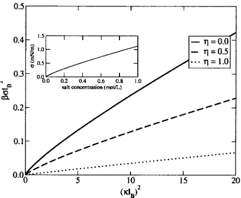
. 共40兲

In Fig. 2, the excess surface tension␴is plotted versus共␬lB兲2

共dimensionless electrolyte concentration兲for different values of ␩. As expected, the excess surface tension increases with increasing ion concentration. This effect is diminished as the dielectric constant of the wall increases leading to a decrease in the screened image charge repulsion. Even when the di-electric constant of the wall and that of the solvent are the same共i.e.,␩= 1兲, the excess surface tension is positive due to the slight exclusion of ions from the interface.

The inset in Fig. 2 shows the excess surface tension in experimentally accessible units, evaluated for a monovalent electrolyte in water at 25 °C共wherelB⬇7 Å兲. This should be

[image:6.612.321.553.46.227.2]

compared with an experimentally measured surface tension of a solution of sodium chloride which is given by␴= 1.6c, wherec is salt concentration in mol/ L, and␴ is in mN/ m. The results presented here underpredict the experimentally observed values, as has been previously observed with simi-lar theories.33The inability of the theory is attributed to using FIG. 1. Ion density distribution for a symmetric electrolyte near a flat inter-face with␬lB= 1 and 共i兲␩= 0 共solid line兲,共ii兲␩= 0.5共dashed line兲,共iii兲

(7)

the bulk screening length near to the interface and to neglect-ing other interactions specific to the nature of the ion, such as ion excluded volume forces,11ionic dispersion interactions,23 or to the structure-making or breaking ability of the ions.34

In the limit that␩Ⰶ1, the expression for the excess in-terfacial tension␴ simplifies to

␤␴= ␬

2

32␲− 2␳

冕

0

⬁

dz

冋

exp

冉

−␤q

2

4⑀ze −2␬z

冊

− 1

册

=␳lB

2

冋

1 2−

2 ␬lB

冕

0

⬁

dtexp

冉

−␬lBe

−t

2t

冊

− 1

册

. 共41兲

Expanding this expression at low electrolyte concentrations yields3

␤␴⬇ ␳lB

2

冋

冉

3

2− 2␥E− ln ␬lB

2

冊

−

冉

␬lB 2

冊冉

ln

␬lB

2 + ln 2 − 2 + 2␥E

冊

+¯

册

, 共42兲 where␥E⬇0.577 215 7 is Euler’s constant. The lowest order

term is precisely the same as that obtained by Onsager and Samaras,3 as well as by Levin, who used an alternate method.33

VI. DIELECTRIC SPHERE IN AN ELECTROLYTE

In this section, we consider a spherical particle of radius

R and dielectric constant ⑀

⬘

immersed in an electrolyte-containing medium共with dielectric constant⑀兲. The electro-lyte is restricted to the outside of the sphere. The Green’s function for this problem is given by 共see Appendix for details兲

G_K共r,r

⬘

兲= e

−␬兩r−r⬘兩

⑀兩r−r

⬘

兩+␦GK共r,r

⬘

兲, 共43兲

where

␦G_K共r,r

⬘

兲= −4␲␬ ⑀

兺

lm

kl共␬r_⬍兲kl共␬r_⬎兲

⫻Dlout共␬R,0,␩兲Ylm共␪,␾兲Ylm* 共␪

⬘

,␾

⬘

兲, 共44兲

␪ is the polar angle of position r,␾is the azimuth angle of positionr,␪

⬘

is the polar angle of positionr

⬘

,␾

⬘

is the azi-muth angle of position r

⬘

,r_⬍ is the radial distance of the position closer to the center of the sphere, andr_⬍is the radial distance of the position further from the center of the sphere. The functionYlmis a spherical harmonic function andDl

out

is given by

Dl

out_共

x,0,␩兲= il共x兲

kl共x兲

冋

l␩−xil

⬘

共x兲/il共x兲

l␩−xkl

⬘

共x兲/kl共x兲

册

. 共45兲

The functions il and kl are the modified spherical Bessel

functions of the first kind and of the second kind, respec-tively.

The ion-interface potential of the mean force is given by

␦G_K共r,r兲= −2␬ ⑀

兺

l=0

⬁

共l+ 1/2兲␬l

2_共␬ r兲Dl

out_共␬

R,0,␩兲. 共46兲

In the absence of screening by other ions 共i.e., ␬= 0兲, the potential of the mean force reduces to the potential of a point charge with its image charges,13,35

␦G_K共r,r兲= − 2 ⑀r

兺

l=1

⬁

␩− 1 ␩+ 1 + 1/l

冉

R r

冊

2l+1

.

[image:7.612.54.294.47.244.2]

The density profile is determined from the ion-interface potential of the mean force 关see Eq. 共35兲兴 which depends only on the ratio of the particle radius to the screening length ␬R. The density profiles for different values of␬Rare plotted in Fig. 3 for the case where␩= 0. In the limit that␬RⰇ1, the correlation lengths in the solvent 共as represented by the screening length兲become small compared with the radius of curvature, and the expression for the self-energy reduces to that found for a planar dielectric interface 关see Eq. 共39兲兴, with z=r−R being the distance from the surface of the sphere. The effect of curvature is important when the radius FIG. 2. Excess surface tension for a symmetric electrolyte at a planar

di-electric interface with␩= 0共solid line兲,␩= 0.5共dashed line兲, and␩= 1共 dot-ted line兲. The inset is for the case where␩= 0 ,lB= 7 Å, andT= 25 ° C.

FIG. 3. Density profile for symmetric electrolytes near a dielectric sphere with␩= 0 ,␬lB= 1, and␬R= 0.01共dashed-dotted line兲,␬R= 0.1共dotted line兲,

[image:7.612.317.555.47.219.2]

(8)

of the particle becomes small compared with the screening length␬R⬍1. For decreasing values of␬R, the magnitude of the screened image interaction is lowered resulting in a de-creased amount of ion desorption. As in the case of the pla-nar geometry, even when the two dielectric constants are identical, there is still an effective repulsion of the ions from the interface.

To evaluate the excess surface tension requires the fol-lowing integral:

−1 2

冕

₀

1

= −

兺

l=0

⬁

共l+ 1/2兲

冕

0

␬R

d␨␨

兵

␨Dl

out_共␨

,0,␩兲关kl

2_共␨兲

−kl−1共␨兲kl+1共␨兲兴−共␬R兲Dlout共␬R,0,␩兲关kl2共␬R兲

−kl−1共␬R兲kl+1共␬R兲兴

其

. 共47兲

This expression was obtained by noting thatK vanishes in-side the dielectric sphere and is a constant outin-side. In addi-tion, we use the second Lommel integral:36

冕

a

⬁

dxx2kl

2_共 x兲= −a

2关kl

2_共

a兲−kl−1共a兲kl+1共a兲兴.

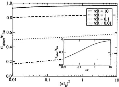
In Fig. 4, the cavity correction factor␴sphere/␴flat共which

is a measure of the influence of curvature on interfacial ten-sion兲is plotted as a function of共␬lB兲2共ion concentration兲at

various values of ␬R for the case where ␩= 0. The cavity correction factor is only a weak function of ion concentration when evaluated at constant ␬R. The correction factor is a much stronger function of ␬R, as also demonstrated by the inset of Fig. 4 where it is plotted versus␬Rfor␬lB= 1. In the

limit that the particle radius becomes large with respect to the screening length 共i.e., ␬RⰇ1兲, ␴sphere/␴flat→1 as

ex-pected because the curved surface appears flat on the scale of the correlation lengths in the solvent. As␬Ris decreased, the cavity correction factor is lowered. This effect can be

attrib-uted to a smaller amount of ion desorption from the curved surface than from the flat surface, which is in agreement with the findings of Groenewold14 for weakly curved dielectric interfaces.

It is insightful to determine the cavity correction factor for a typical protein, such as lysozyme共with a radius of 15Å兲 dissolved in an aqueous solution of monovalent ions. For salt concentrations ranging from 0.1, to 1.0M the values of ␬R

range from about 1.5 to 5, and according to Fig. 4, this would correspond to correction factors between 0.8 and 0.95, respectively.

The microscopic equivalent of electrolyte adsorption at an interface is the protein-salt preferential interaction parameter—the difference in the salt molality in the domain of the protein over that in bulk. Arakawa and Timasheff1 have measured this parameter for lysozyme or bovine serum albumin共BSA兲in various salt solutions. The experimentally observed parameters are within a factor of about 0.7 of those values calculated assuming the protein is a low dielectric body with no curvature. In this case, the preferential interac-tion parameter can be calculated from the molal surface-tension increment of the salt. The reason that there is less exclusion of salt about a protein than as predicted using this assumption was attributed to specific interactions between the salt and the protein surface.

We have shown that increasing the curvature of the pro-tein surface will slightly decrease salt exclusion. While this effect is not large enough to entirely account for the discrep-ancy with the experimentally observed preferential interac-tion parameters, it does indicate that the dominant forces that control the exclusion of the salt about the protein surface are similar to those that control the distribution of ions about a low dielectric cavity. In dilute electrolyte solutions, the ex-clusion of the salt is driven primarily by 共 geometry-dependent兲 image charge interactions, which the above theory incorporates. For more concentrated salt solutions, however, other factors need to be included such as ion ex-cluded volume,11ion dispersion forces,23 or forces resulting from the structure-making or breaking ability of the ion.34

VII. CONCLUSIONS

A variational theory was developed and applied to study the properties of electrolyte solutions at dielectric interfaces. The particular cases of planar and spherical geometries were examined. The advantage of this approach over the standard Poisson-Boltzmann equation is that it includes ion-ion corre-lation effects. Also, because we work directly with a free energy, the need to integrate the Gibbs adsorption equation is avoided and thermodynamic consistency is ensured.

[image:8.612.54.292.47.222.2]

For the planar case, the ions preferentially desorb from the interface. There are two contributions to the potential of the mean force between an ion and the interface: a screened image charge interaction and a repulsive force originating from exclusion of the electrolytes from the dielectric wall. The lower the dielectric constant of the interface, the more strongly the ions desorb, and consequently, the larger the excess surface tension. Even when the dielectric constant of the interface is the same as in the bulk, the ions still desorb FIG. 4. Ratio of the excess surface tension for a dielectric sphere with

⑀⬘Ⰷ⑀immersed in a symmetric electrolyte and surface tension for a planar

interface:␬R= 0.01共solid line兲,␬R= 0.1共dashed line兲,␬R= 1共dotted line兲,

and␬R= 10共dashed-dotted line兲. The inset shows the variation of the excess

(9)

from the interface, resulting in a positive excess surface ten-sion. At low electrolyte concentrations, the excess surface tension predicted by the variational theory reduces to the Onsager-Samaras limiting law.3

For spherical dielectric particles, the excess surface ten-sion decreases as the particle radius decreases. In the limit that the radius of the sphere becomes much larger than the Debye screening length, the properties of the system reduces to that of a planar dielectric interface.

In this work, we only have examined symmetric electro-lytes. If there are any differences between the negative and positive charge carriers 共e.g., a different valence or specific interaction with the interface兲, then this asymmetry will lead to charge separation and the generation of a potential differ-ence between the dielectric particle and the bulk electrolyte solution. In addition, we have neglected the presence of non-electrostatic interaction between particles. These interactions can be included by using a reference state grand partition function Z_Gref other than the ideal-gas reference state 共e.g., the Carnahan-Starling equation of state37 can be used to in-clude exin-cluded volume interactions24兲. This approach can also be used to include specific interactions between the ions and the interface. This is especially important to study the Hofmeister effect where the surface tension depends on the specific nature of the ion. These nonelectrostatic interactions can also lead to the enhanced adsorption of highly polariz-able ions at low dielectric interfaces.38 Consequently, other ion specific interations such as ion-dispersion interactions and effects due to ion hydration need to be included in surface tension models to better understand the Hofmeister effect.

APPENDIX: GREEN’S FUNCTION FOR THE STURM-LIOUVILLE PROBLEM

In this Appendix, we develop the Green’s function asso-ciated with the screening function given in Eq. 共31兲 for spherical geometries. The Green’s function G_K is given by the solution of

⑀共r兲

4␲

冋

− 1

⑀共r兲ⵜ ·⑀共r兲ⵜ +␬ 2_共_r_兲

册

_G

K共r,r

⬘

兲=␦d共r−r

⬘

兲, 共A1兲 where ⑀共r兲 is the spatially varying dielectric constant, and ␬共r兲 is the spatially varying inverse screening length. The Green’s function can be expanded in a series involving the spherical harmonicsYlm,

G_K共r,r

⬘

兲=

兺

lm

gl共r,r

⬘

兲Ylm共␪,␾兲Ylm

* _共␪

_⬘

,␾

⬘

兲. 共A2兲

Substituting this expansion into the Green’s function equa-tion yields

⑀共r兲

4␲r2

冋

−

1 ⑀共r兲

⳵ ⳵rr

2_⑀共_r_兲⳵

⳵r+l共l+ 1兲+r

2_␬2_共_r_兲

册

_g

l共r,r

⬘

兲

= 1

r2␦共r−r

⬘

兲. 共A3兲

For the system considered in this work, the dielectric

con-stant and the screening length are concon-stant within the droplet and outside the droplet, although they are discontinuous across the two regions. If we focus on one of these regions, the Green’s function problem reduces to

⑀ 4␲r2

冋

−

⳵ ⳵rr

2⳵

⳵r+l共l+ 1兲+r 2_␬2

册

_g

l共r,r

⬘

兲=␦共r−r

⬘

兲.

共A4兲

For this one-dimensional problem, the Green’s function is simply given by39

gl共r,r

⬘

兲= −

1

C

再

u共r兲␷共r

⬘

兲forr⬍r

⬘

u共r

⬘

兲␷共r兲forr⬎r

⬘

,

冎

共A5兲

where u and ␷ are solutions of the corresponding homoge-neous differential equation, which is

⑀ 4␲r2

冋

−

d drr

2d

dr+l共l+ 1兲+r

2_␬2

册

_y_共_r_兲_{= 0,} _共_A6_兲

and its solutions are linear combinations of modified, spheri-cal Bessel functionsil共r兲 andkl共r兲, which are defined as

il共x兲=

冉

␲ 2x

冊

1/2

Il+1/2共x兲=

共x/2兲l

⌫共l+ 1兲 1 2

冕

₋₁

1

dt共1 −t2兲le−xt,

kl共x兲=

冉

2 ␲x

冊

1/2

Kl+1/2共x兲=

共x/2兲l ⌫共l+ 1兲

冕

₁

⬁

dt共t2− 1兲le−xt, whereIlandKlare the modified Bessel functions of the first

and second kinds, respectively.

The general solution of the homogeneous differential equation can be written as a linear combination of the two independent solutions,

u共r兲=Auil共␬r兲+Bukl共␬r兲,

␷共r兲=A_␷il共␬r兲+B␷kl共␬r兲,

whereAu,Bu,A␷, and B␷ are constants chosen such that the

solution u satisfies the lower boundary condition, and the solution␷satisfies the upper boundary condition.

Inside the sphere共i.e., r⬍R兲, it is assumed that the in-verse Debye screening length is ␬2 and the dielectric

con-stant is⑀2. Outside the sphere, it is assumed that the inverse

Debye screening length is␬1and the dielectric constant is⑀1.

u共r兲=

再

Au 共2兲_i

l共␬2r兲 r⬍R Au共1兲il共␬1r兲+B共u1兲kl共␬1r兲 r⬎R,

冎

共A7兲

␷共r兲=

再

A␷ 共2兲_i

l共␬2r兲+B␷共2兲kl共␬2r兲 r⬍R B_␷共1兲kl共␬1r兲 r⬎R.

冎

共A8兲

The functions u and␷must be continuous. In addition, the displacement vector must also be continuous. Applying these conditions to the function u yields the following equations:

Au共

1兲_i

l共␬1R兲+Bu共

1兲_k

l共␬1R兲=Au共

2兲_i

(10)

Au共

1兲_⑀

1␬1il

⬘

共␬1R兲+Bu共

1兲_⑀

1␬1kl

⬘

共␬1R兲=Au共

2兲_⑀

2␬2il

⬘

共␬2R兲.

共A10兲

For this scale, we choose A_u共2兲= 1. Using the following identity:39

il共x兲kl

⬘

共x兲−il

⬘

共x兲kl共x兲 ⬅−

1

x2, 共A11兲

these equations can be inverted to give explicit expressions for A_u共1兲 andB_u共1兲,

Au共

1兲_{= −}共␬1R兲2

⑀1␬1

关⑀1␬1kl

⬘

共␬1R兲il共␬2R兲

−⑀2␬2il

⬘

共␬2R兲kl共␬1R兲兴, 共A12兲 Bu共1兲=

共␬1R兲2

⑀1␬1

关⑀1␬1il

⬘

共␬1R兲il共␬2R兲−⑀2␬2il

⬘

共␬2R兲il共␬1R兲兴.

共A13兲 Similarly for the function␷, we have

B_␷共1兲kl共␬1R兲=A␷共2兲il共␬2R兲+B␷共2兲kl共␬2R兲, 共A14兲 B_␷共1兲⑀1␬1kl

⬘

共␬1R兲=A␷共2兲⑀2␬2il

⬘

共␬2R兲+B␷共2兲⑀2␬2kl

⬘

共␬2R兲.

共A15兲

Choosing the scale of␷ by setting B_␷共1兲= 1, the solutions of the above equations are

A_␷共2兲= −共␬2R兲

2

⑀2␬2

关⑀2␬2kl

⬘

共␬2R兲kl共␬1R兲

−⑀1␬1kl共␬2R兲kl

⬘

共␬1R兲兴, 共A16兲 B_␷共2兲=共␬2R兲

2

⑀2␬2

关⑀2␬2il

⬘

共␬2R兲kl共␬1R兲−⑀1␬1il共␬2R兲kl

⬘

共␬1R兲兴.

共A17兲

The constantCis related39to the Wronskian of Eq.共A6兲,

C=p共x兲W共x兲

=p共x兲关u共x兲␷

⬘

共x兲−u

⬘

共x兲␷共x兲兴

= R

2

4␲关⑀1␬1kl

⬘

共␬2R兲kl共␬1R兲兴. 共A18兲

The Green’s function is then given by

gl共r,r

⬘

兲= −

4␲

R2

⫻关Auil共␬r⬍兲+Bukl共␬r⬍兲兴关A␷il共␬r⬎兲+B␷kl共␬r⬎兲兴

⑀1␬1kl

⬘

共␬2R兲kl共␬1R兲

,

共A19兲

wherer_⬎共r_⬍兲is the larger共lesser兲of the two radial distances

r and r

⬘

. When both the vectors r and r

⬘

lie outside the sphere, the Green’s function reduces to

gl共r,r

⬘

兲=

4␲␬1

⑀1

关il共␬1r⬍兲

−Dlout共␬1R,␬2R,␩兲kl共␬1r⬍兲兴kl共␬1r⬎兲, 共A20兲

where

Dl

out_共

x1,x2,␩兲= il共x1兲 kl共x1兲

⫻

冋

⑀2x2il

⬘

共x2兲/il共x2兲−⑀1x1il

⬘

共x1兲/il共x1兲

⑀2x2il

⬘

共x2兲/il共x2兲−⑀1x1kl

⬘

共x1兲/kl共x1兲

册

.

共A21兲

In the situation where there is no salt inside the sphere共i.e., ␬2= 0兲,

Dlout共x,0,␩兲=

il共x兲

kl共x兲

冋

l␩−xil

⬘

共x兲/il共x兲

l␩−xkl

⬘

共x兲/kl共x兲

册

. 共A22兲

Substituting these expressions into the series expansion for the Green’s function yields the following:

G_K共r,r

⬘

兲=4␲␬1 ⑀1

兺

lm

il共␬1r⬍兲kl共␬1r⬎兲 ⫻

冋

1 −Dlout共␬1R,␬2R,␩兲

kl共␬1r⬍兲

il共␬1r⬍兲

册

⫻Ylm共␪,␾兲Ylm* 共␪

⬘

,␾

⬘

兲=

e−␬1兩r−r⬘兩

⑀1兩r−r

⬘

兩

−4␲␬1 ⑀1

兺

lm

kl共␬1r⬍兲kl共␬1r⬎兲 ⫻Dl

out_共␬

1R,␬2R,␩兲Ylm共␪,␾兲Ylm

* _共␪

_⬘

,␾

⬘

兲. 共A23兲

The first term is the Green’s function of a bulk electrolyte. The second term represents the influence of the dielectric particle. The corresponding expression for␦G_Kis

␦G_K共r,r兲= −2␬1 ⑀1

兺

l=0

⬁

共l+ 1/2兲kl2共␬1r兲Dlout共␬1R,␬2R,␩兲.

共A24兲

1_{T. Arakawa and S. N. Timasheff, Biochemistry} _{21, 6545}_共₁₉₈₂_兲_.

2_{C. Wagner, Phys. Z.} _{25, 474}_共₁₉₂₄_兲_.

3_{L. Onsager and N. T. Samaras, J. Chem. Phys.} _{2, 528}_共₁₉₃₄_兲_.

4_{D. Bratko, B. Jönsson, and H. Wennerström, Chem. Phys. Lett.} _{128, 449}

共1986兲.

5_{R. Kjellander and S. Mar}_č_{elja, Chem. Phys. Lett.} _{112, 49}_共₁₉₈₄_兲_.

6_{R. Kjellander and S. Marcelja, J. Chem. Phys.} _{82, 2122}_共₁₉₈₅_兲_.

7_{R. R. Netz, Phys. Rev. E} _{60, 3174}_共₁₉₉₉_兲_.

8_{T. Croxton, D. A. McQuarrie, G. N. Patey, G. M. Torrie, and J. P.}

Valleau, Can. J. Chem. 59, 1998共1981兲.

9_{G. M. Torrie, J. P. Valleau, and G. N. Patey, J. Chem. Phys.} _{76, 4615}

共1982兲.

10_{G. M. Torrie, J. P. Valleau, and C. W. Outhwaite, J. Chem. Phys.} _81,

6296共1984兲.

11_{L. B. Bhuiyan, D. Bratko, and C. W. Outhwaite, J. Phys. Chem.} _{95, 336}

共1991兲.

12_{P. Linse, J. Phys. Chem.} _{90, 6821}_共₁₉₈₆_兲_.

13_{R. Messina, J. Chem. Phys.} _{117, 11062}_共₂₀₀₂_兲_.

(11)

15_{A. L. Kholodenko and A. L. Beyerlein, Phys. Rev. A} _{34, 3309}_共₁₉₈₆_兲_.

16_{R. D. Coalson and A. Duncan, J. Chem. Phys.} _{97, 5653}_共₁₉₉₂_兲_.

17_{J. Ortner, Phys. Rev. E} _{59, 6312}_共₁₉₉₉_兲_.

18_{R. R. Netz and H. Orland, Eur. Phys. J. E} _{1, 203}_共₂₀₀₀_兲_.

19_{R. R. Netz, Eur. Phys. J. E} _{3, 131}_共₂₀₀₀_兲_. 20_{R. R. Netz, Eur. Phys. J. E} _{5, 189}_共₂₀₀₁_兲_.

21_{D. S. Dean and R. R. Horgan, Phys. Rev. E} _{69, 061603}_共₂₀₀₄_兲_.

22_{A. M. Walsh and R. D. Coalson, J. Chem. Phys.} _{100, 1559}_共₁₉₉₄_兲_.

23_{M. Boström, D. R. M. Williams, and B. W. Ninham, Langmuir} _{17, 4475}

共2001兲.

24_{L. Lue, N. Zoeller, and D. Blankschtein, Langmuir} _{15, 3726}_共₁₉₉₉_兲_.

25_{J.-P. Hansen and I. R. McDonald,}_{Theory of Simple Liquids}_{, 2nd ed.}

共Academic, London, 1986兲.

26_{J. D. Jackson,}_{Classical Electrodynamics}_共_{Wiley, New York, 1975}_兲_.

27_{R. L. Stratonovich, Dokl. Akad. Nauk SSSR} _{115, 1097}_共₁₉₅₇_兲_.

28_{J. Hubbard, Phys. Rev. Lett.} _{3, 77}_共₁₉₅₉_兲_.

29_{R. P. Feynman,} _{Statistical Mechanics: A Set of Lectures} _共

Addison-Wesley, Redwood, CA, 1972兲.

30_{R. R. Netz and H. Orland, Eur. Phys. J. E} _{11, 310}_共₂₀₀₃_兲_.

31_{H. Kleinert,}_{Path Integrals in Quatum Mechanics, Statistics, and Polymer}

Physics, 2nd ed.共World Scientific, Singapore, 1995兲.

32_{J. L. Lebowitz and J. K. Percus, J. Math. Phys.} _{4, 116}_共₁₉₆₃_兲_.

33_{Y. Levin, J. Chem. Phys.} _{113, 9722}_共₂₀₀₀_兲_.

34_{M. Manciu and E. Ruckenstein, Adv. Colloid Interface Sci.} _{105, 63}

共2003兲.

35_{J. M. Caillol, D. Levesque, and J. J. Weiss, J. Chem. Phys.} _{91, 5544}

共1989兲.

36_{G. N. Watson,} _{A Treatise on the Theory of Bessel Functions}_{, 2nd ed.}

共Cambridge University Press, Cambridge, 1944兲.

37_{N. F. Carnahan and K. E. Starling, J. Chem. Phys.} _{51, 635}_共₁₉₆₉_兲_.

38_{P. B. Petersen, R. J. Saykally, M. Mucha, and P. Jungwirth, J. Phys.}

Chem. B 109, 10915共2005兲.

39_{G. Arfken,}_{Mathematical Methods for Physicists}_{, 3rd ed.}_共_{Academic, San}