MICHAEL MALEY
JANUARY 1982
A THESIS SUBMITTED FOR THE DEGREE OF MASTER OF ARTS
Acknowledgements
I wish to thank David Band, Clive Bean, Arthur Burns, David Butler, Paul Collits, John Curtice, Brian Embury,
Peter Hall, C.R. Heathcote, Lady Kendall, Chandran Kukathas, Colin Mackenzie, Koula Mellos, P.A.P. Moran and David
Sankoff for suggestions, criticisms, comments and encourage ment from which I have benefited in the work leading to the preparation of this thesis.
I also wish to express my gratitude to all those who attended the seminars in the Department of Political Science, Faculty of Arts, ANU, at which some of this material first
surfaced. In particular I would like to thank those who attended out of friendship rather than interest.
To three people I owe special thanks. William Maley gave considerable assistance with the joyless task of proof reading; his goal of achieving immortality on this page has been reached.
Malcolm Mackerras first stimulated my interest in the study of elections, and has been a constant and generous source of material and intellectual aid over the years. I wish to record my particular appreciation of this.
CONTENTS
CHAPTER ONE - INTRODUCTION (1)
I (1)
II (6)
III (8)
IV (25)
V (27)
VI (30)
VII (33)
FOOTNOTES TO CHAPTER ONE (35)
CHAPTER TWO - PENDULUM MODELS (57)
I (57)
II (58)
III (59)
IV (64)
V (71)
VI (73)
VII (77)
VIII (89)
IX (93)
X (100)
FOOTNOTES TO CHAPTER TWO (103)
CHAPTER THREE - ANALYSES BASED ON REGRESSION (118)
I (118)
III (120)
IV (123)
V (137)
VI (142)
FOOTNOTES TO CHAPTER THREE (144)
CHAPTER FOUR - MISCELLANEOUS APPROACHES (151)
I (151)
II (151)
III (158)
IV (161)
FOOTNOTES TO CHAPTER FOUR (162)
CHAPTER FIVE - CONCLUSIONS (164)
APPENDIX I (171)
APPENDIX II (173)
APPENDIX III (175)
Chapter One - Introduction
There is no greater gamble on earth than a British general election - James Middleton, 1936
The British electoral system is not a gamble...the relation between a party 1 s representation in Parliament and its support in the country is almost as predictable as it would be under proportional representation - David Butler,
1953
I
One of the most widely discussed concepts in the study of voting and elections has been electoral bias. This thesis has two purposes. The first is to develop a number of meas ures of bias so as to avoid the defects inherent in those measures which have hitherto been in popular use. The second
is to analyse the measures so developed from a critical viewpoint. ^
The term "bias" can be interpreted broadly or narrowly. In its broadest sense "bias" could encompass any aspect of the electoral process which advantages one or more candid ates or parties, such as, for example, the differential
2
impact of informal voting, or of the "donkey vote". But the measures considered in this thesis are based on a much
3
seats. Henceforth "bias" will be regarded as the extent to which the relationship between seats and votes differs from party to party. When "bias" is so defined, the political
significance of its discovery is immediately clear. For a number of popular measures of bias, this is not the case. Johnston, for example, puts forward a measure based on
Hacker's well-known classification of votes as "effective", "excess" or "wasted".^ However, a positive value of this
measure does not by itself even imply that the proportion of seats which will be won with a given proportion of the total vote will vary from party to party. The principles of polit
ical equality which are breached in such a situation remain vague and unspecified, and it is thus appropriate that our definition should exclude such measures.
Such an approach carries with it a recognition of the central role played by political parties in the legislative politics of most liberal democracies. In this thesis we consider only measures of bias against political parties
(rather than including, if there be any, measures of bias against individual candidates). This approach can be defend ed on a number of different grounds.
From a theoretical standpoint, it can first be argued that an electoral system need not involve individual candid ates. Conceivably voters might be offered only a choice between two or more parties; this is true even in a case
current system, the people choose an electoral college, and the electors in that college choose the President. But the system could also work if the electors in the college were replaced by appropriate tokens, such as discs of different colours (or elephants and donkeys), which could be counted to determine the outcome of the election. This of course represents a polar situation in which the role of the indiv idual candidate is completely eliminated by institutional factors. The theoretical possibility of such a system makes it worthy of study in its own right.
Secondly it can be argued that where there are only single-member constituencies, it is meaningless to talk of bias against an individual candidate, since the concept of bias which we have adopted relates only to the relationship between the total proportion of the vote polled by a party and the total proportion of the seats which it wins, and since the outcome of the election in a specific seat is causally prior to, and logically independent of, both of these quantities. Under Australian electoral law, it is possible for a candidate to contest every seat in the legis
lature. Under such circumstances, however, it is more appropriate for our purposes to regard him as a party
(albeit a small one).
As well as these theoretical arguments, there is empir ical evidence in the Australian case to support an exclusive emphasis on the position of parties. A number of studies in Australia have made clear the extent to which voters iden
degree of influence which this has on the way in which they vote.^ These are complemented by a study which finds that in Australia the impact of the individual candidate on the out
come of elections at the state and federal level has been • • i 6
minimal.
Some analysts have argued that the fate of political parties at elections is only of secondary importance, and have preferred to analyse the manner in which the electoral
system takes account of the preferences of the individual voter.^ This approach, in deflecting attention from the
fates of parties, takes insufficient account of the way in which parties have become the major routes of interest
articulation for the great bulk of voters in many countries. Because of this trend, the distinction between the way in which the. system treats the voter and the way in which it
treats his or her party is a somewhat artificial one. Finally in defence of this approach, it should be
pointed out that concentration on the fates of parties is a major feature of the substantial literature on electoral bias which already exists
Even with this restriction, our perspective is still too broad. It will be narrowed further by limiting consider ation to those electoral systems marked by single-member constituencies, and the plurality or preferential methods of scrutiny. In practice this is not very restrictive, since the electoral systems for the lower houses of the Australian Federal Parliament, the Australian Mainland State
Parlia-g
U.S. Congress fall into these categories. Numerical examples from past elections for some of these houses will be used from time to time in this thesis. It is also worth noting that it is in the context of single-member constituencies that bias has been most frequently discussed in the previous literature.
In addition, the decomposition of measures of bias according to its alleged causes will not be attempted. The detection of the most frequently mooted of these causes -malapportionment and gerrymandering - is a relatively simple
9
matter, which has been well canvassed in the literature.
Finally, the significance of the word measure should be emphasised. By this it is implied that the figures produced are expressible in the same units as the disadvantage im posed on the handicapped party. It is also possible to produce indices of bias, such as the correlation of the percentage votes for a party in the various constituencies and the enrolments in those constituencies,^ but these are outside the scope of this study.
In the evaluation of measures of electoral bias, three broad criteria are applied - logical soundness, empirical acceptability, and statistical simplicity.
is the requirement that measures be based on valid empirical assumptions. A measure can be criticized if it is based on assumptions which are either universally invalid or unduly restrictive; such criticisms will respectively destroy a measure, or seriously limit its applicability. Finally, it
is desirable that measures be simple to calculate and easy to interpret.
These criteria will be applied hierarchically. The first quality required of a measure must always be logical soundness, and the other criteria need only be applied to measures which pass this initial test. The criterion of
simplicity is an important one, since measures which are difficult to interpret are unlikely to prove very useful to political scientists. In the last resort, however, this
criterion must be regarded as subsidiary, and the virtue of simplicity can never compensate for failings on logical or empirical grounds.
II
Reference was made in the first paragraph of Section I to "defects inherent in those measures which have hitherto been in popular use". The existence of these defects was
established by the present writer in an earlier w o r k . ^ Some of the arguments advanced in that work must now be reiterated in a condensed form, to establish clearly the need for the analysis which follows, and to introduce a number of key concepts which provide a framework for that analysis.
Gudgin and Taylor (in 1974), by Soper and Rydon (in 1958), 12
and by Butler (in 1947) . All are based explicitly on the assumption of single-member constituencies, each contested by only two candidates, bearing the standards of the two political parties which exist in the postulated polity. The assumption of a pure two-party system is a restrictive one, although less so in the case of Australian elections than in the case of those in, for example, Great Britain or New
Zealand, for in Australia in the vast majority of constit uencies the Labor and L-NCP candidates unequivocally achieve
the best and second-best results in the final count, which allows meaningful (though naturally error-prone) estimates
13
of a "two-party preferred vote" to be made. The pure two- party situation, despite its distance from reality, requires detailed consideration, for theorizing on electoral matters largely proceeds heuristically, and if the simplest possible state of affairs cannot be rigorously analysed, there will exist no platform from which to launch more ambitious invest igations. Some analysts might choose to attack these measures p u r e l y because they are based on the two-party assumption.^ Such an approach, however, would leave their validity in an actual two-party situation unchallenged. The critique about to be offered is thus more general, and therefore more damag ing, than such an approach.
"For any given proportion of the overall vote3 the same proportion of seats should he wons whichever party is concerned" . ^
When this is not fulfilled, there exists what Butler calls "bias", what Gudgin and Taylor call "partisan bias", and what Soper and Rydon call "under-representation". This
definition of "bias" has a clear appeal, but it does exhibit one slightly paradoxical aspect, namely that it classifies as unbiased a situation in which there is a negative relat ionship between seats and votes, that is, in which either party can win more than half of the seats while winning less than half of the total vote.
In the following sections, two main propositions are established. The first is that Gudgin and Taylor, and Soper and Rydon, err by basing their measures respectively on the calculation of "non-partisan bias" and the "effective vote", when both are inherently unquantifiable. The second is that
Butler's measure is based on the empirically untenable
assumption that in the event of a non-uniform swing in votes from one party to the other, the same number of seats will change hands as would have been the case had the swing been uniform.
Ill
Gudgin and Taylor set out in a general form a measure 16 which has been used extensively in Australia and elsewhere.
constituencies. They first note that the proportion of seats won by a party under such a system is rarely the same as its proportion of the vote. On the basis of this they define
"electoral bias” as the difference between these two propor tions. They next observe that the winning party's proportion of the seats typically exceeds its proportion of the v o t e . ^ From this they conclude that there exists some systematic factor advantaging a party which wins a majority of the vote, which they encapsulate in the equation:
(1.1) PS/(1-PS) = f[OV/(l-OV)]
where PS and OV are respectively the proportion of seats and 18 of the overall vote won by the party under consideration. For practical purposes, Gudgin and Taylor use a less general equation:
(1.2) PS/U-PS) = [OV/(l-OV)]a
19 where a is a number greater than or equal to zero. By
solving this equation for PS and subtracting OV, we obtain what Gudgin and Taylor call "non-partisan bias" (NPB)
"sinee it accrues to either party depending on which one
20
wins a majority or minority of votes". Put formally:
(1.3) NPB = {(OV)“/[(OV)a+(l-OV)a]} - OV
bias" constitutes "partisan bias" (PB). This is the quantity of main significance. This is formally expressed as:
(1.4) PB = PS - {(0V)“/ [(0V)a+(l-0V)a] }
These concepts are most easily conveyed diagrammatically:
Diagram (1.1)
"Electoral", "Partisan" and "Non-Partisan Bias"
Proportion of Seats
0.5 OV
Proportion of Overall Vote
equation (1.2) for some value of a greater than zero. The distance AC represents "electoral bias", the distance AB represents "non-partisan bias", and the distance BC repres ents "partisan bias".
Clearly, "electoral bias" is known, since we know the proportion of seats and votes won by each party. So the
calculation of "partisan bias" requires the discovery of the value of a in equation (1.4). It should be pointed out at this stage that the derived value of "non-partisan bias" is very sensitive to variations in the value of a. This is
illustrated in the following table, which sets out values of PS derived from equation (1.2) for various values of OV and a :
a
Table
1
(1.1)
2 3 4
OV
0.50 0.50 0.50 0.50 0.50
0.51 0.51 0.52 0.53 0.54
0.52 0.52 0.54 0.56 0.58
0.53 0.53 0.56 0.59 0.62
0.54 0.54 0.58 0.62 0.66
0.55 0.55 0.60 0.65 0.69
0.56 0.56 0.62 0.67 0.72
variation of 0.04 in the derived value of PS. The exponent a must be specified with considerable accuracy.
Although there is no obvious reason for doing so, a number of analysts, including Gudgin and Taylor, proceed by
21
attributing to a a value of three. For them, this follows from a belief in the so-called "cube law", which must now be examined in some detail. The modern popularity of the "cube law" originated in an article by David Butler in "The
Econ-22
omist" in January, 1950, which was subsequently elaborated by Kendall and Stuart in a classic paper published in the
23
same year. For Kendall and Stuart, the "law" is an observed empirical regularity , without any particular normative
implications:
"The law3 briefly 3 states that the proportion of seats won by the victorious party varies as the cube of the proportion of votes cast for that party over the country as a whole"
After making some adjustments for minor party candidacies, they find that the "cube law" describes well the results of the British general elections of 1935 and 1945.
Kendall and Stuart's investigation of the possible causes of this empirical regularity uses a frequency histo gram of the proportion of the combined Labour and Conserv ative vote in each seat polled by the party winning the election. Gudgin and Taylor, who also adopt this approach, refer to such a histogram as the "constituency proportion
25
Diagram (1.2)
The Constituency Proportion Distribution
Number of Seats
Proportion of Vote
Each rectangle represents one constituency. In this case, the winning party has won 53 seats, and the losing party has won eight seats. As the number of constituencies increases, this discrete distribution approaches a continuous form, which is mathematically more convenient to manip
ulate . ^
Kendall and Stuart assume that electoral swing will take the form of a "sliding" of the entire CPD along the horizon tal axis, so that its shape is unchanged, and prove that if this is so, the "cube law" will hold, provided that the CPD is approximately normal, with a standard deviation of
27
0.137 . They emphasise that the "law" is merely an empir ical pattern:
fact that the distribution of proportions p_ at an election is nearly normal3 (b) the mathematical fact that the cubic-proportion law very closely approximates to a normal form with the same vari ance and (c) the empirical fact the the variance of the cubic-proportion law is very closely approx imated by the variance of the observed distribut ions . The law is thus not universal"
This passage can be interpreted in two ways. It can be viewed as advancing a model of the "cube law" as briefly defined earlier, that is, a set of sufficient (though not necessary) conditions for the cubic seats-votes relationship to hold. Alternatively, it can be seen as a new and more restrictive definition of the "cube law". The distinction is an import ant one, because the alternative interpretations give rise to different strategies of empirical testing. The broader version of the "law" can be tested by examining the propor
tions of seats and votes gained by a party at one or more elections, whereas to test the narrower version, the CPDs which actually occur must be looked at. The latter approach
is adopted by Kendall and Stuart, and the trend towards a narrow interpretation of the meaning of the "cube law" has continued in much of the subsequent literature.
The "law" has been tested empirically by Kendall and Stuart themselves, Butler, Gudgin and Taylor, March, Tufte, Linehan and Schrodt, Brookes, Soper and Rydon, Sankoff and
29
only to illustrate the difficulties which they encounter. Tufte fits a logit regression model to seats-votes data from seven polities, and rejects the "cube law" hypothesis
30
for six of them. Linehan and Schrodt re-estimate the para meters using a non-linear regression procedure, and obtain
31
results much more favourable to the "law” . In a note published in 1979, Laakso obtains results which are "too
32
ambiguous for a general interpretation” , and which vary according to the degree of disaggregation of the analysis, and the number of parties considered. Taken as a whole,
these studies are quite ambivalent about the "cube law", and reflect the limited empirical support which it has received in the literature.
However, from the standpoint of justifying the choice of three as a value for a, these studies are irrelevant. What is required to provide such a justification is not empirical evidence supporting the "cube law", but a theory implying that in the absence of partisan bias, a cannot take any value but three. Much confusion arises from the failure to make this crucial distinction.
At first glance this point might appear to be a simple consequence of "Hume's Law" - that one cannot deduce a norm ative precept from a set of pure statements of positive facts - but this in fact is not the case; for Gudgin and Taylor, non-partisan bias is itself a real, objective phen-
33
observed, and there is no logical reason for making such an assumption. This is so even if CPDs, rather than total seats and votes at a number of elections, are examined. Although Gudgin and Taylor see each possible value of a as being
isomorphically related to a particular symmetrical CPD, even a symmetrical CPD can be seen as merely a deviation from another symmetrical CPD which in some sense is the '’real” , ’’underlying” distribution.^^
Gudgin and Taylor appear to see models of the gener ation of a CPD with the variance required for the "cube law” to hold as constituting theories of the type which we have seen are necessary. Such models are advanced by Kendall and
35
Stuart, March, and Gudgin and Taylor themselves. We shall briefly look at them all.
Kendall and Stuart put forward two tentative ideas. The first is a Markov chain model, in which constituencies are produced by drawing samples from the total electorate. The sampling process, however, displays the property that succ essive choices are correlated, so that if a voter for party A is chosen at a given draw, it is highly likely that a voter
for party A will also be chosen at the next draw. This can
36
be formally expressed as follows:
Let P(A|A) be the probability that if a voter from party A is drawn, the next voter drawn will also be from party A.
Let P(A|B) be the probability that if a voter from
Let gß be the proportion of party A voters in the total electorate.
Let g be a random variable, the proportion of votes for party A in equal-sized constituencies of T voters.
Kendall and Stuart point out that as T approaches infinity, the probability distribution of g approaches the
37 normal distribution, with mean gg and variance given by:
(1.5) Var (g) = [gQ (l-gQ) (1+e)] / [t (1-e)]
Two aspects of the model are important. First, it must be noted that it only gives the asymptotic probability distrib ution of the random variable g. It does not guarantee that
the empirical CPD produced by such a scheme will be normal (in the sense defined in footnote 27). However, it can be said that for large values of T, the probability of the CPD . deviating substantially from normality will be small, and there is some evidence to suggest that for this particular
3 8 scheme, convergence to normality is quite rapid.
Secondly, it is clear that to produce a variance
sufficient to explain the "cube law", e must be very close to one for typical values of T. Kendall and Stuart point out that for T = 60,000 (a typical constituency size), the model
39
requires that e - 0.9995. This implies a similar high value for P(A|A), and a very low value for P(A|B), since P(A|B) £ 0, and P(A I A) < 1.
samples are drawn is divided into perfectly homogeneous
spatial clusters, of a precise average size determined by the 40
values of gQ and T. For g^ = 0.5, and T = 60,000, clusters 41
of about 5,000 voters are required. But this makes the model highly implausible in many cases. In the Australian
context, for example, the most cursory scrutiny of sub- divisional returns for elections for the Commonwealth House of Representatives makes clear that there are no parts of the country sufficiently politically homogeneous to fulfil the requirements of the model. This empirical implausibility leads Kendall and Stuart to discount the value of their
Markov model.
The second model involves what is known as a Lexian sampling scheme. Constituencies are regarded as random sam ples from larger sub-groups of the overall electorate. Each
constituency consists of voters taken entirely from one sub group, and each sub-group contributes equally to the total number of samples. We let g^ be the probability that a voter taken from the ith sub-group votes for party A. The random variable g again is asymptotically normally distributed, with variance given b y : ^
(1.6) Var(g) = [gQ (l-g0) + (T-l).Var(g^)]/T
With T large, Var (g) - Var(g^.).
upon the variance of , and thus can model other "laws". It therefore does not provide an adequate justification for the choice of three as a unique value for a.
March's model sees the CPD as a synthesis of two hypo thetical distributions, one unimodal and reflecting broad scale inter-party decisions regarding factors such as cam paign resource allocation across the constituencies, and the
other bimodal, reflecting such factors as varying voter enthusiasm and despair in safe and marginal seats.^ This model is criticised in detail by Gudgin and Taylor.^ For our purposes, we need merely note that its generation of a "cube law" CPD depends crucially upon the fortuitous occurr ence of particular values of a number of exogenous para meters. Alternative values of these parameters can produce a normal CPD with a different variance, and can even produce a
45
Poisson CPD. The model is therefore open to precisely the same criticism as that directed at Kendall and Stuart's
Lexian scheme, and thus fails to justify the choice of three as a value for a.
Gudgin and Taylor put forward four models. The first two are based on binomial sampling schemes, are put forward only for didactic purposes, and are incapable of producing a CPD with a sufficiently high variance for the "cube law" to
46
hold. The third is a variant of Kendall and Stuart's Lexian model, in which g^ is assumed to be a random variable with a
two-parameter beta distribution. Under such a scheme, the value of the term "Var(g^.)" in equation (1.6) is determined
However, there is no prior reason for assuming that these parameters can only take values which will ensure the prod uction of a CPD with the "cube law" variance, and for this reason Gudgin and Taylor's Lexian scheme fails on the same grounds as that of Kendall and Stuart.
The fourth model, upon which Gudgin and Taylor place most emphasis, is a development of Kendall and Stuart's Markov chain scheme. Constituencies are created by the ran
dom choice of clusters of voters , rather than individuals.^ Two types of clusters are postulated. One is a "working
class" cluster, in which the proportion of party A voters is equal to w. The other is a "middle class" cluster, in which
49
the proportion of party B voters is equal to w . We denote by T the equal numbers of voters in each constituency, and by c the equal number of voters in each cluster. The variance of the resulting random variable g is given by:"*^
(1.7) Var (g) = [(2w-l) 2gQ (l-g0)c (1+e)] (1-e)
52
"cube law" variance. They argue that the model:
"can he viewed as both an explanation of the cube law and as setting up a standard form against whiah
53
actual CPDs may be compared".
In its role as a standard form, the model is not susceptible to empirical testing. Its validity must therefore depend on the extent to which its major structural features have
analogues in the real world. Here it falls down in two main respects. It does not allow for variations in the sizes of constituencies or clusters, which limits its applicability. More importantly, it assumes that clusters are discrete and homogeneous. The difficulty arises in the identification of clusters as the basic units of analysis, notwithstanding the fact that at any given election the pattern of clustering which actually occurs is the result of the voting decisions
of the individual electors. Now with a free ballot, the possibility of considerable fluctuations in clustering patt erns from election to election must be admitted. But in such a confused situation, the boundaries of clusters, and there fore their sizes, become ill-defined, and Var(^) becomes meaningless. This seriously undermines the claim that the model provides "a standard form against which actual CPDs may be compared". For these reasons, it must be regarded as
inadequate for our purposes.
Apart from the preceding models based on the CPD, a number of other models of the "cube law" have been put
This approach has been criticized in detail by Gudgin and
55
Taylor; its inadequacy for us lies in the fact that its central concept is a purely hypothetical one, with no ana logue in the actual system of vote scrutiny.
56 A rather different approach is taken by Theil. His model is based on a decomposition of the vote in each seat
into a local constituency effect, and an overall election effect. However, Theil explicitly assumes that for a given swing in the overall vote, the swing to the party gaining will be greatest in its previously weakest seats, and least in
its previously strongest s e a t s T h i s assumption is an intuitively appealing one, but as a foundation of a general explanation of the "cube lawM , it is rendered dubious by contrary evidence. The issue is discussed at some length by Butler and Stokes, who point out that at the five British elections from 1951, swing at the constituency level appears to be relatively independent of the initial level of party
5 8
support. Since Britain has been found in several studies to be that polity which most closely conforms to the "cube law", this observation is particularly damaging to Theil's
59
model. Taagepera also notes that the model may only work well when the division of total votes between the two parties
is approximately even, since otherwise the error terms in a number of Taylor series approximations in Theil's proof
60 become unacceptably large.
Quandt examines the "cube law" through the application of an impressive stochastic model of voting, based on the
61
model is a general one, which produces the "cube law" as an asymptotic outcome when a number of probability distribution parameters conveniently occur. For this reason, Quandt's analysis cannot justify the exclusive choice of three as a value for a.
In this brief survey of the literature, no adequate support for the choice of three as a value for a in equation
(1.4) has been found. Some analysts have put forward models which imply different values for a. Sankoff and Mellos, for example, demonstrate through the application of game theory that:
"If the parties in a two-party system could freely allocate their total support among the constit uencies 3 we should expect a swing ratio equal to
. „ 62 two .
They further suggest that the swing ratio associated with the "cube law" will be generated if one third of the voters are "hard core". In a subsequent article, Sankoff reaches a similar conclusion for a situation in which party resources are partially fixed in some districts, by applying the game
6 3
of "Blotto". The major problem with these models, conceded by Sankoff and Mellos, is that the assumption that parties
can freely decide the distribution of their votes is unreal istic. At best, party control of vote distributions occurs through media of the type discussed by March, which are so crude and unpredictable in their effects as to render their use for "fine tuning" impossible.
Taagepera must be considered. He suggests that the exponent a is equal to the ratio of the natural logarithms of the number of voters (v) and the number of seats (n) in the
polity under consideration. He notes that when v = n, a = 1, which represents a case of extreme proportional represent ation, and that when n = 1, a = °°, which represents a case of direct presidential election. Reasoning from a postulated two-stage electoral process, Taagepera derives the
equat-64 ion:
(1.8) a(v ,n) = m(y)/m(n)
There are two flaws in nis line of reasoning. First, he admits that there is no "clear cut proof" that the function
6 S m( ) in equation (1.8) is the natural logarithmic function.
Secondly, he assumes that a depends only on the number of 66
voters and seats. While this is true in the unrealistic boundary cases on which he relies, it is not obviously true in cases where the number of seats is much greater than one, but much less than the number of voters. Taagepera offers no argument in support of this assumption. These defects make Taagepera's approach an unsatisfactory one.
But to use Gudgin and Taylor's measure, a value for a must be specified. So far, we have accepted the assumption that this can be done. This must now be challenged. To do this, equation (1.1) must be looked at rather more closely. The implication of this equation is that a certain propor
purely as a result of the overall proportion of the vote which it wins. Gudgin and Taylor equate this with a situat
ion in which the CPD is symmetrical. For each possible value of a, there exists a corresponding symmetrical CPD.
Gudgin and Taylor's approach, therefore, involves see ing the skewed CPDs which actually occur as deviations from one of these symmetrical CPDs. But CPDs are produced by a multitude of individual voting decisions. The act of specify
ing a unique value for a constitutes an assertion that had votes not been cast in the pattern in which they were, they
could have been cast in only one other pattern so as to produce a symmetrical CPD. But such an assertion is unten
able. Had the people not voted as they did, there is no
logical way of knowing for certain how they would have voted. The problem, therefore, is not that a value of a exists but cannot be discovered; it is that the very idea of a unique value for a is absurd. With single-member constituencies,
there simply can never be a functional relationship between overall proportions of seats and votes, and it is absurd to proceed on the basis that we can know what this relationship would be if it existed.
Non-partisan bias is thus clearly revealed as a concept which for purely logical reasons cannot be quantified. The measure of partisan bias put forward by Gudgin and Taylor must therefore be set aside.
IV
6 7
Rydon. This has proved to be very popular in Australian psephology, and has also been noted in a number of overseas
68
studies. They propose as a measure of "under-representation" the difference between the overall proportion of the vote
obtained by a party, and the "effective vote" for that 69
party. By the "effective vote", Soper and Rydon mean that vote for a party which would have produced the actually ob served division of seats if partisan bias (as defined by - Gudgin and Taylor) had not been present.^ This concept once again can be conveyed diagrammatically:
Diagram (1.3) The Effective Vote
In this diagram, the curve OBX represents a particular ’’standard of exaggeration of majorities” (or to use Gudgin and Taylor’s terminology, a specific level of non-partisan bias). ’’Under-representation” is given by OV - OV^. The
symmetry of this measure and that of Gudgin and Taylor is immediately obvious. The same assumptions and empirical propositions underlie both, but in Soper and Rydon’s
measure, the decision is made to measure bias in terms of' votes rather than seats.
The main defect in their measure is simply that it is not possible to specify a unique "effective vote” . The argument that demonstrates this follows directly from that mounted against Gudgin and Taylor's measure. "Under
representation” is conceded by Soper and Rydon to be a function of the pattern of votes cast. To postulate a dis coverable "effective vote” is to argue that it is possible to discover the pattern in which votes would have been cast had they not been cast in the pattern in which they were. The absurdity of this has already been pointed out. Since an election can logically be viewed as a deviation from any number of possible "standards of exaggeration of majorities”
there are also any number of "effective votes” , one for each possible "standard” ; the idea of a unique "effective vote” is therefore absurd. On the basis of this, it can be seen that Soper and Rydon's measure is ill-founded.
V
Butler in the early Nuffield election studies. He deduces from the CPD of an individual election a curve giving the division of seats associated with each possible division of the vote. He does this by noting the number of seats which would fall to uniform swings of different sizes. From this
curve, the division of seats at a 50-50 division of the vote can be read, and the divergence of this seat division from a 50-50 split constitutes the level of bia s . ^
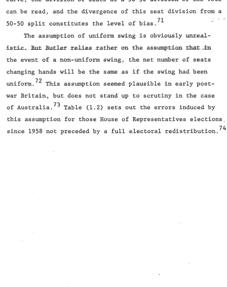
The assumption of uniform swing is obviously unreal istic. But Butler relies rather on the assumption that in the event of a non-uniform swing, the net number of seats changing hands will be the same as if the swing had been
72
uniform. This assumption seemed plausible in early post war Britain, but does not stand up to scrutiny in the case
73
[image:33.563.74.528.233.808.2]Table (1.2)
Year Benefit to ALP of non-uniform swing (seats)
Swing to
A L P (7o)
Std. dev. of swing
1958 -1 -0.32 3.5
1961 6 4.65 3.4
1963 0 -3.14 3.3
1966 -1 -4.34 4.4
1972 2 2.50 4.2
1974 1 -1.01 3.5
1975 -3 -7.38 2.7
1980 -2 4.20 3.0
The figures in the second column are obtained by subtracting from the number of seats actually won by the ALP the number of seats which the ALP would have won had the swing been uniform. The mean absolute error is two seats, or about 1.67» with a maximum error of six seats, or 4.917», in 1961. It is
also apparent that there is some positive correlation between the error occurring at a particular election, and the swing at that election.^
Although these data alone provide a counter-example to Butler's assumption, two other recent cases are worthy of mention. The first is the South Australian general election
of 1979. A uniform swing would have given the non-Labor side of politics 24 seats. In fact, the non-Labor parties won 27
7 6
[image:34.563.89.523.72.428.2]particularly striking because a prominent opposition member, Mr Ren de Garis, relying on Butler's methodology, had accused
the ALP government of perpetrating a "vicious gerrymander".^ The second case to note is the New Zealand general election of 1978. At that election, Labour won six fewer seats than
78 it would have won with a uniform swing, an error of 6.52%.
These tests of Butler's empirical assumption might be thought to be unnecessarily severe, and indeed Butler only claims approximate accuracy for his "empirical formulas". To this two responses can be made. The first is that there is no clearly defined point at which a formula's predictions cease to be approximately accurate. The second is that the degree of accuracy required of such formulas must vary accor ding to their application. If they are to be used, for
example, to interpret public opinion polls during an election campaign, a prediction error of five or six seats may be
tolerable. But when bias is being measured, very much greater accuracy is required. If the size of bias figures is small, say two or three seats, the possibility of prediction errors
7 9 of the order of six seats completely destroys their value. It is for this reason that great importance must be attached to the counter-examples just cited. They lead ineluctably to the conclusion that Butler's approach is inadequate.
VI
Let us now take stock of the argument to this point. Three popular measures of bias have been examined and found
common element in the defectiveness of all three, which strikes at the very heart of the concept of bias upon which they are based. Recall the norm set out by Soper and Rydon:
"For any given proportion of the overall vote3 the same proportion of seats should be won3 whichever party is concerned".
Now for any election, the proportion of seats achieved by the winner is known. But the proportion of seats which the loser would have obtained with the same vote can never be known, for as has been made clear, this is not a uniquely
deter-80
minable proportion, but a random variable. This is a fact with which Gudgin and Taylor, and Soper and Rydon, never
adequately cope, while Butler tries to deal with it by the adoption of an unrealistic empirical assumption.
It follows from this that the statistics described and analysed so far in this chapter are not even measures as the term has been defined. Since the seats-votes relationship is a stochastic one, differences in this relationship from party to party take the form of differences in the chances which the various parties have of winning a specified proportion of the seats with a given proportion of the vote. Measures of bias must reflect this fact.
replacement of the norm used by Soper and Rydon. It can be required that:
For any given proportion of the overall vote3 the probabilities of the various possible divisions of
the seats should be the same for all parties. Rather less stringently, it can be required that:
For any given proportion of the overall vote3 the expected number of seats won should be the same for all parties.
The former implies the latter; the converse is not true. The precise manner in which these norms are translated into
measures of bias depends on the statistical techniques in use. A detailed defence of the use of probabilistic models
in the analysis of electoral processes is set out by Niemi 81
and Weisberg.
One final point should be made. In the most popular axiomatization of probability theory, that of Kolmogorov, "probability" figures as a primitive, undefined concept, and the interpretation to be placed on numerical
probabil-8 2
ities has been a matter of vigorous philosophical dispute. Henceforth, when we refer to the probability that an
individual, constituency or nation votes in a particular way, we shall take this to be a measure of an objective propensity for such an outcome to occur. This view, put forward by Karl
8 3
voting clearly falls).^ This interpretation is implicit in 85
the terminology used by Gudgin and Taylor, and provides a framework into which such concepts as the strength of party allegiance, and the safety of seats, can be translated.
VII
The remainder of this thesis will be concerned with the development of some probabilistic measures of bias.
In the second chapter, it is shown that an assumption that the vote won by a party in each seat is an independent random variable implies a stochastic seats-votes relation
ship. Initially within the framework of a two-party assump tion, it is shown that a measure of bias can be calculated easily if the probability distributions of the government's proportion of the vote in each seat can be specified. The bulk of the chapter considers this specification problem in detail, and it is concluded that plausible, though not
objectively correct, specifications can be provided. Some limitations to the plausibility of such specifications are noted, and finally the measure is formulated to cope with a multi-party situation. It is argued that the measure devel oped is a simple and useful one.
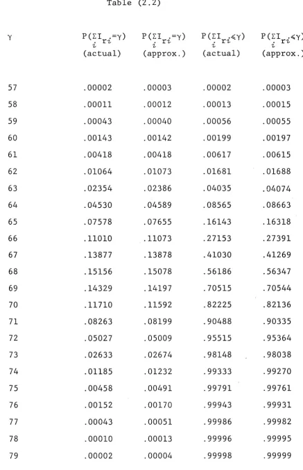
In the third chapter, the application of the two- variable linear regression model to the problem of bias measurement is considered. The empirical validity of the
circumstances are identified in which derived bias figures will be invalid, and it is argued that subject to this
limitation the measure of bias produced is a useful one. The fourth chapter considers two analyses, which model the seats-votes relationship probabilistically without
proposing direct empirical measures of bias. It is shown that measures of bias can, in fact, be derived from these analyses; it is further shown, however, that they are less useful than the measure derived in Chapter Two, since they share its pitfalls and in addition are much more difficult to apply practically.
In conclusion, it is argued that the measures of bias produced do avoid the problem that haunts the previous
literature; that the investigator in choosing between the measures of Chapters Two and Three must be guided both by
the data available and the extent to which their respective underlying assumptions are fulfilled; and that the measures, when appropriately used, are sound and useful tools for
The following items in the literature have considerable theoretical significance: R.H. Brookes, "The Analysis of Distorted Representation in Two-Party Single Member Elections", Political Science , 12, 2, 1960, pp 158-67; D. E. Butler, "The Relation of Seats to Votes", in R.B. McCallum and A. Readman, The British General
Election of 1945, Oxford University Press, London, 1947; G. Gudgin and P.J. Taylor, "Electoral Bias and the
Distribution of Party Voters", Transactions of the Institute of British Geographers, 63, 1974, pp 53-74; G. Gudgin and P.J. Taylor, Seats3 Votes3 and the Spatial Organisation of Elections, Pion, London, 1979; G. Gudgin and P.J. Taylor, "The Decomposition of Electoral Bias in a Plurality Election", British Journal of Political Science, 10, 1980, pp 515-21; R.J. Johnston, Political3 Electoral3 and Spatial Systems, Clarendon Press, Oxford, 1979; A.G. Pulsipher, "Empirical and Normative Theories of Apportionment", Annals of the New York Academy of Sciences , 219, 1973, pp 334-41; R.E. Quandt, "A Stoch astic Model of Elections in Two-Party Systems", Journal of the American Statistical Association, 69, 1974,
pp 315-24; C.S. Soper and J. Rydon, "Under-
Review, 67, 1973, pp 540-54.
2. For studies of such phenomena, see G. Snider, "The Partisan Component of the Informal Vote", Politics ,
14, 1979, pp 82-8; and M. Mackerras, "Preference Voting and the 'Donkey Vote' ", Politics , 5, 1970, pp 69-76.
3. This process, under the title "Conversion into Patterns of Representation", appears in both taxonomies of
electoral geography put forward in R.J. Johnston, "Electoral Geography and Political Geography",
Australian Geographical Studies , 18, 1980, pp 37-50.
4. R.J. Johnston, Political3 Electoral3 and Spatial
Systems, pp 63-7; A. Hacker, Congressional Districting , rev. ed., The Brookings Institute, Washington D.C., 1964, pp 54-61.
5. D. Aitkin, Stability and Change in Australian Politics , Australian National University Press, Canberra, 1977, ch. 3; D.A. Kemp, Society and Electoral Behaviour in Australia, University of Queensland Press, St. Lucia,
1978, p 362.
6. M. Mackerras, Incumbency as an Electoral Advantage,
7. This approach is particularly prevalent among advocates of proportional representation. A typical example is
K.N. Grigg, "The Value of a Voter", Australian Quarterly , 41, 1, 1969, pp 52-9. Grigg uses the vote taxonomy put forward in Hacker, Congressional Districting, which has, however, been critically examined in R.J. Sickels,
"Dragons, Bacon Strips and Dumbbells - Who's Afraid of Reapportionment?", Yale Law Journal, 75, 1966, pp 1300- 8, and in P. Musgrove, "The General Theory of Gerry mandering", Sage Professional Papers in American Politics , 3, Series no. 04-034, 1977, pp 21-3.
8. The lower house in NSW now uses optional preferential voting.
9. See Musgrove, "The General Theory of Gerrymandering". There are many different measures of malapportionment in popular use. My own favourite is that proposed by H.F. Kaiser, "A Measure of the Population Quality of Legislative Apportionment", American Political Science Review, 62, 1968, pp 208-15, which varies between zero and one.
10. C.A. Hughes, "Fair and Equal Constituencies: Australia, Jamaica and the United Kingdom", Journal of Commonwealth and Comparative Politics , 16, 1978, pp 256-71 at p 267.
sub-thesis, Department of Political Science, Faculty of Arts, Australian National University, 1979.
12. Gudgin and Taylor, "Electoral Bias and the Distribution of Party Voters"; Soper and Rydon, "Under-Representation and Electoral Prediction"; Butler, "The Relation of
Seats to Votes". Maley, Five Measures of Electoral Bias, also examines measures proposed in Brookes, "The
Analysis of Distorted Representation in Two-Party Single Member Elections", and in Tufte, "The Relationship
between Seats and Votes in Two-Party Systems". Brookes's work is not specifically analysed in this thesis, since
the criticisms offered of Butler's measure apply equally and directly to Brookes's . Tufte's work is considered from a different viewpoint in a later chapter.
13. The concept of the "two-party preferred vote" is expl ained in M. Mackerras, Elections 1975, Angus & Robertson, Sydney, 1975, pp 3-6, and defended in M. Mackerras,
"Rejoinder to Campbell Sharman", Politics, 13, 1978, pp 339-42. Data supporting the assertion of the meaning
fulness of two-party preferred vote estimates are provided in Maley, Five Measures of Electoral Bias,
unpredictable factor into the notional allocation of preferences, and as a consequence the reliance which is placed on such estimates must be reduced.
14. This is one line of criticism put forward in Maley,
Five Measures of Electoral Bias, pp 60-73.
15. Soper and Rydon, "Under-Representation and Electoral' Prediction", p 94. A similar criterion, referred to
as "neutrality", is proposed by R.G. Niemi and J. Deegan, "A Theory of Political Districting", American Political
Science Review, 72, 1978, pp 1304-23.
16. For example, see C.A. Hughes, "The Electorate Speaks -and After", in H.R. Penniman (ed.), Australia at the
Polls - The Rational Elections of 1975, American
Enterprise Institute for Public Policy Research,
Washington D.C., 1977, pp 277-311 at p 287; D. Jaensch, "A Functional 'Gerrymander' - South Australia, 1944- 1970", Australian Quarterly, 42, 4, 1970, pp 96-101 at p 99; J. Kelly, "Vote Weightage and Quota Gerrymanders in Queensland, 1931-1971", Australian Quarterly , 43, 2, 1971, pp 39-54 at p 51.
17. Support for these propositions can be found in D.W. Rae,
and votes under single-member constituencies was known to the early French probabilists. See C.C. Heyde and E. Seneta, I.J. Bienayme - Statistical Theory Anticip ated, Springer-Verlag, Berlin, 1977, pp 106-8.
18. In "Electoral Bias and the Distribution of Party Voters", p 54, Gudgin and Taylor give an incorrect version of this equation, with votes as the dependent variable. It should be noted that the notation used when reproducing equations in this thesis is rarely the
same as that used by the original authors, since consid erable modifications are necessary to avoid the confus ion which arises when different authors use the same symbols to stand for different quantities.
19. H. Theil, "The Desired Political Entropy", American Political Science Review, 63, 1969, pp 521-5, considers
a situation in which OV is the proportion of the total vote polled by a party, and PS is the proportion of
seats which it wins. He proves that if PS./PS. =
v y
f(0V./0V.), if the same relationship holds for all i,y,
v J
and if f( ) is a continuous, non-decreasing function which takes positive values for all positive values of
the argument, then f( ) must be of the form (0V./0V.)a ,
v y
l-f(l-OV^). The proof is reproduced in H. Theil, Statistical Decomposition Analysis, North Holland, Amsterdam and London, 1972, pp 96-7.
20. Gudgin and Taylor, "Electoral Bias and the Distribution of Party Voters", p 55.
21. Ibid., p 69; Gudgin and Taylor, Seats3 Votes3 and the Spatial Organisation of Elections , p 87; Hughes, "The Electorate Speaks - and After", p 287; Jaensch, "A Functional 'Gerrymander1 - South Australia, 1944-1970", p 99; Kelly, "Vote Weightage and Quota Gerrymanders in Queensland, 1931-1971", p 51.
22. [p.E. Butler], "Electoral Facts", The Economist, 158, 5550, January 7, 1950, pp 5-7. Butler points out his authorship of this article in A. Stuart, N.L. Webb and D. Butler, "Public Opinion Polls", Journal of the Royal Statistical Society3 Series A, 142, 1979, pp 443-67 at p 456.
23. M.G. Kendall and A. Stuart, "The Law of the Cubic Proportion in Election Results", British Journal of Sociology , 1, 1950, pp 183-96.
24. Ibid., p 183.
Gudgin and Taylor, Seats, Votes, and the Spatial
Organisation of Elections , ch. 2 et seq. It was first introduced in this context by F.Y. Edgeworth, ’’Miscell aneous Applications of the Calculus of Probabilities", Journal of the Royal Statistical Society, Series A, 61, 1898, pp 534-44.
26. Gudgin and Taylor, Seats, Votes, and the Spatial Organisation of Elections , p 15.
27. It should be noted that: (i) the assumption of a "slid ing" distribution is not the same as an assumption of "uniform swing" ("swing identical in every seat"). For Kendall and Stuart, "swing" denotes the mean change in
the proportion of the vote won by the party under consideration in each constituency. The "mean swing" will equal the "overall swing" ("change in the propor
tion of the total vote polled by the party under consid- ation") if the swing is uniform, or if at each election, for every seat, the ratio of the number of votes cast to the total number of votes in all seats is equal to 1/n, where n is the number of seats, (ii) When we describe the CPD as "normal", we are merely asserting that the frequencies of the various vote proportions are closely approximated by the function:
where \i is the mean vote proportion achieved by the party under consideration, and a is the empirical
standard deviation of the CPD. (iii) Gudgin and Taylor,
Seats3 Votes3 and the Spatial Organisation of Elections,
p 28, point out that in the critical regions the ’’cube law" is slightly better approximated by a normal
distribution with a standard deviation of 0.133.
28. Kendall and Stuart, "The Law of the Cubic Proportion in Election Results", p 191.
29. M.G. Kendall and A. Stuart, "La Loi du Cube dans les Elections Britanniques", Revue Francaise de Science
Foliti.que, 2, 1952, pp 270-6; Kendall and Stuart, "The Law of the Cubic Proportion in Election Results";
D.E. Butler, "Appendix: An Examination of the Results",, in H.G. Nicholas, The British General Election of 1950, Macmillan, London, 1951, pp 328-9; D.E. Butler, The
British General Election of 1951, Macmillan, London, 1952, pp 275-6; D.E. Butler, The Electoral System in
Britain 1918-1951, Oxford University Press, London,
1953, pp 192-4; Gudgin and Taylor, Seats3 Votes3 and the
Spatial Organisation of Elections , p 25; J.G. March, "Party Legislative Representation as a Function of Election Results", in P.F. Lazarsfeld and N.W. Henry
Systems"; W.J. Linehan and P.A. Schrodt, "A New Test of the Cube Law", Political Methodology , 4, 1977, pp 353— 67; R.H. Brookes, "Seats and Votes in New Zealand: The Butler Analysis and the Cube Law", Political Science, 5, 2, 1953, pp 37-44; R.H. Brookes, "Legislative Representation and Party Vote in New Zealand: Reflec
tions on the March Analysis", Public Opinion Quarterly , 23, 1959, pp 288-91; Soper and Rydon, "Under-
Representation and Electoral Prediction"; D. Sankoff and K. Mellos, "La Regionalisation Electorale et
1 'Amplification des Proportions", Canadian Journal, of Political Science , 6, 1973, pp 380-98; M. Laakso,
"Should a Two-and-a-Half Law Replace the Cube Law in British Elections?", British Journal of Political
Science, 9, 1979, pp 355-62; R.S. Robins, "Votes, Seats, and the Critical Indian Election of 1967", Journal of Commonwealth and Comparative Politics , 17, 1979,
pp 247-62.
30. Tufte, "The Relationship between Seats and Votes in Two-Party Systems", p 546.
31. Linehan and Schrodt, "A New Test of the Cube Law", pp 358-60.
33. Gudgin and Taylor, Seats, Votes 3 and the Spatial Organisation of Elections , pp 86-91.
34. Ibid., pp 64-8. See also P.J. Taylor and R.J. Johnston, Geography of Elections , Penguin, Harmondsworth, 1979, pp 392-6.
35. Kendall and Stuart, "The Law of the Cubic Proportion in Election Results", pp 195-6; J.G. March, "Party
Legislative Representation as a Function of Election Results"; Gudgin and Taylor, Seats, Votes, and the Spatial Organisation of Elections , pp 31-53, 205-21.
36. Kendall and Stuart, "The Law of the Cubic Proportion in Election Results", p 195. Gudgin and Taylor, Seats3
Votesj and the Spatial Organisation of Elections , pp 40-2, also deals with this model.
37. For the derivation of this formula, Kendall and Stuart refer their readers to J.V. Uspensky, Introduction to Mathematical Probability , McGraw-Hill, New York and London, 1937, pp 223, 301.
38. Ibid., p 229.