Classification algorithms on the cell processor

Rochester Institute of Technology

RIT Scholar Works

Theses Thesis/Dissertation Collections

8-1-2008

Classification algorithms on the cell processor

Mateusz Wyganowski

Follow this and additional works at:http://scholarworks.rit.edu/theses

This Thesis is brought to you for free and open access by the Thesis/Dissertation Collections at RIT Scholar Works. It has been accepted for inclusion in Theses by an authorized administrator of RIT Scholar Works. For more information, please [email protected].

Recommended Citation

Classification Algorithms on the Cell Processor

by

Mateusz Wyganowski

A Thesis Submitted in Partial Fulfillment of the Requirements for the Degree of Master of Science in Computer Engineering

Supervised by

Dr. Muhammad Shaaban Department of Computer Engineering

Kate Gleason College of Engineering Rochester Institute of Technology

Rochester, NY August 2008

Approved By:

_____________________________________________ ___________ ___

Dr. Muhammad E. Shaaban

Primary Advisor—R.I.T. Dept. of Computer Engineering

_ __ ___________________________________ _________ _____

Dr. Juan C. Cockburn

Secondary Advisor—R.I.T. Dept. of Computer Engineering

_____________________________________________ ______________

Dr. Roy W. Melton

Abstract: The rapid advancement in the capacity and reliability of data storage technology has

allowed for the retention of virtually limitless quantity and detail of digital information. Massive

information databases are becoming more and more widespread among governmental,

educational, scientific, and commercial organizations. By segregating this data into carefully

defined input (e.g.: images) and output (e.g.: classification labels) sets, a classification algorithm

can be used develop an internal expert model of the data by employing a specialized training

algorithm. A properly trained classifier is capable of predicting the output for future input data

from the same input domain that it was trained on.

Two popular classifiers are Neural Networks and Support Vector Machines. Both, as with most

accurate classifiers, require massive computational resources to carry out the training step and can

take months to complete when dealing with extremely large data sets. In most cases, utilizing

larger training improves the final accuracy of the trained classifier. However, access to the kinds

of computational resources required to do so is expensive and out of reach of private or under

funded institutions.

The Cell Broadband Engine (CBE), introduced by Sony, Toshiba, and IBM has recently been

introduced into the market. The current most inexpensive iteration is available in the Sony

Playstation 3 ® computer entertainment system. The CBE is a novel multi-core architecture

which features many hardware enhancements designed to accelerate the processing of massive

amounts of data. These characteristics and the cheap and widespread availability of this

technology make the Cell a prime candidate for the task of training classifiers.

In this work, the feasibility of the Cell processor in the use of training Neural Networks and

Support Vector Machines was explored. In the Neural Network family of classifiers, the fully

connected Multilayer Perceptron and Convolution Network were implemented. In the Support

Vector Machine family, a Working Set technique known as the Gradient Projection-based

Chapter 1: Introduction ... 5

1.1 The Problem Domain... 5

1.2 Classifiers... 5

1.3 The Cell Broadband Engine... 6

1.4 Organization... 6

Chapter 2: Multi Layer Perceptron ... 8

2.1 Chapter Introduction ... 8

2.2 Background ... 8

2.3 The Neuron Model... 9

2.4 The Linear Separator... 10

2.5 Learning Algorithms... 12

2.6 Training the Multi Layer Perceptron ... 18

2.7 Network Architecture... 25

2.8 Convolutional Networks ... 26

2.9 Related Work ... 27

Chapter 3: Support Vector Machines... 28

3.1 Chapter Introduction ... 28

3.2 Background ... 28

3.3 Training... 28

3.4 Implementations... 35

3.5 Conclusion ... 51

Chapter 4: The Cell Broadband Engine ... 53

4.1 Chapter Introduction ... 53

4.2 Design Challenges ... 53

4.3 Top Level Design... 54

4.4 Low Level Design Decisions ... 56

4.5 Power Processing Element... 57

4.6 Synergistic Processing Elements ... 58

4.7 Floating Point Number Representation... 61

4.8 Element Interconnect Bus ... 62

4.9 Memory Interface... 63

4.10 Previous Work on Cell Processor ... 64

Chapter 5: High Performance Programming on the Cell Processor ... 65

5.1 Chapter Introduction ... 65

5.2 Support and Development Tools ... 65

5.3 CBE Embedded SPE Object Format... 70

5.4 Levels of Programming... 71

5.5 Programming the PPE... 80

Chapter 6: Implementation of the Multi-Layer Perceptron on the Cell Processor ... 82

6.1 Chapter Introduction ... 82

6.2 High Level Implementation Overview ... 83

6.3 Detailed Implementation... 85

Chapter 7: Implementation of Support Vector Machines on the Cell Processor... 110

7.1 Chapter Introduction ... 110

7.2 Parallel Gradient Projection-based Decomposition Technique ... 110

Chapter 8: Test Methodology and Results... 144

8.1 Chapter Introduction ... 144

8.2 Multi Layer Perceptron ... 146

8.3 Gradient Projection-Based Decomposition Technique... 153

8.4 Other Results... 158

Chapter 9: Conclusion and Future Work ... 159

9.1 Chapter Introduction ... 159

9.2 Multilayer Perceptron ... 159

9.3 Gradient Projection-based Decomposition Technique ... 160

9.4 Cascade SVM... 160

Chapter 1: Introduction

1.1 The Problem Domain

The strong and steady improvement in data storage technology has lead to an abundance of data being stored by virtually every existing organization. E-commerce companies store transaction details on a per-customer basis. Amazon, for example, generates

millions of transactions per day. National Security organizations may collect information about suspected and unsuspected individuals such as travelers or internet users. Banks collect information about their customers which includes spending habits, credit dept and transaction histories. Google, which specializes in data storage, collects information about every search term and every link clicked by every user. Most companies log some portion of incoming and outgoing packet data between their internal intranet(s) and the internet.

There is a lot of valuable information within this data – the problem lies in extracting it. It should be possible, for example, for a bank to predict a new customer’s likelihood to go bankrupt by studying all previous similar customers in terms of specified attributes. An advanced intrusion detection system may use a sequence of incoming packets along with timing information to detect novel incoming network attacks. A large e-commerce company may use the data as an aid in choosing which advertisements to show based on the current logged in user (or browser cookie received). The problem is how to search this massive data and create a knowledge model so that future examples from the same domain are classified into some predefined set of classes.

1.2 Classifiers

This is one problem in which classification algorithms, or classifiers, excel. These mathematical tools work by taking as input a set of features of an object, situation, or a piece of data and to producing as an output a discreet value which denotes that input’s class. In order to do so, an associated training algorithm is used to generate an internal classifier model, or knowledge, using previous input/output pairings from the same source (problem) domain. This process of building an internal prediction model is known as Data Mining or Machine Learning.

possible to conclude that the chosen parameters have produced an optimal classifier however. The multiple algorithms and variations available, the parameter adjustability, and most importantly the computational intensity for training make it difficult to explore all possibilities within a reasonable amount of time.

The most popular classification algorithms are the Neural Network (of which the

Multilayer Perception is most utilized), Support Vector Machines, k-Nearest Neighbours, Gaussian, Naïve Bayes, Decision Tree and RBF classifiers. This work is concerned with the first two (Multilayer Perceptrons and Support Vector Machines).

1.3 The Cell Broadband Engine

The Cell Broadband Engine Architecture (Cell for short) was released in 2005 by Sony, Toshiba, and IBM. The processor consists of one Power Processor Element, and nine Synergistic Processor Elements (six of which are accessible on the Playstation 3® system used in this work) on one chip tied with a high speed ring bus. The architecture features various novelties that suggest exceptional performance. However, in order to achieve this performance, programs for the Cell Processor need to be explicitly written to take

advantage of the hardware. Issues of memory latencies, reformatting of data, workload distribution, all the way down to instruction scheduling need to be carefully considered. The Playstation 3® is arguably the best performance-per-dollar system available due to marketing and business reasons.

The goal of this work is to implement and explore the performance of a two novel Support Vector Machine implementations – the Parallel Gradient Projection-Based Decomposition Technique (PGPDT) and Cascade SVM along with the standard Multi-layer Perceptron and a recent Convolution Layer Neural Network architectures on the Cell Broadband Engine Architecture.

1.4 Organization

The document was written with the assumption that it will be read in order and can be logically divided into four main sections.

Chapters 2 and 3 make up the first section and introduce the two classifiers, placing detail into the variations that are relevant to this work. It is recommended that even those readers familiar with MLPs and SVMs read the sections describing the relatively new MLP convolution layers, and the sections about the novel GPDT working set method and cascade SVM solvers.

The next section, consisting of Chapters 4 and 5, changes course and is concerned with the Cell Broadband Engine and the programming strategies for writing high performance applications on the said architecture. The programming strategies were included in a separate chapter due to the significance that they played in this work.

used as much as possible to convey the concepts, especially where pushing, storage, or processing of data is concerned.

Chapter 2: Multi Layer Perceptron

2.1 Chapter Introduction

In this chapter, the Multilayer Perceptron – the most popular member of the Artificial Neural Network (ANN) family – is introduced.

The chapter begins by introducing the basic building block of any ANN – the single Neuron model. This less technical section is broken into the most significant

developments and improvements leading up to this day. Details covered are kept within the scope of this work.

The following sections increase in technicality and expand on the concepts introduced in the first section. First, the Single-Layer Perceptron is dissected along with its learning methodology. Next, the Multi-Layer Perceptron is examined by expanding on the Single-Layer version.

Next, the Backpropagation method – the heart of the training power of the MLP – is explained both mathematically and intuitively. Here, the pitfalls and shortcomings of the algorithm, as well as the many variations and parameters that attempt to reduce them are further elaborated.

Typical implementations of the algorithm on modern computer architectures, the feasibility of parallelization, and some recent work are discussed in the next section.

Finally, the convolution layer is described. This layer type was designed to outperform a standard fully-connected layer when 2-dimensional images are the source of the training data.

2.2 Background

Two types of layers were implemented in this work – the fully-connected layer and the convolution layer. In the fully-connected layer each neuron on a layer has a separate dedicated weighted connection to each neuron on the previous layer provided that it is not the input layer. A convolution layer consists of a number of two-dimensional feature maps, each paired with a kernel that is used to generate the values of the feature map by performing a kernel pass over all of the previous layer’s feature maps. While in the more general case it is possible to select which feature maps to process for each feature map on the given layer, the implementation in this work processes all input feature maps for each one.

The learning algorithm used in the MLP is known as Backpropagation, which is a gradient descent method having the goal of minimizing an error function at the output layer generated by feeding the network with elements from the training set. The

optimization variables are the weights in the fully-connected layers and kernel elements in the convolution layers.

2.3 The Neuron Model

The Artificial Neuron is the basic building block of the MLP. The theory behind the MLP

can be better understood by first obtaining an intuition into the theory behind the single neuron.

The first neuron model was proposed by McCulloch and Pitts in 1943 [2]. This

biologically inspired computational model (from hereon referred to as the M-P model) was very basic, capable of functioning only with binary inputs and outputs. Over the years, the original M-P model has received various modifications from the fields of statistics and probability theory which have allowed it to be applied to a broader range of problems. The modern revision of the neuron unit is shown in Fig. 2-1.

Figure 2-1: The Artificial Neuron Model

arrow is used to represent the bias b, the purpose of which will be discussed later. There are two steps that are taken to calculate the scalar output x. The first step involves calculating the activation value z as a function of the input vector and weight vector. Most commonly, z is calculated by taking a weighted sum of all the inputs (a dot product of the weight and input vector). The result is input to an activation function F(.) to produce the final output x. For the neuron in the figure, the two steps are summarized by:

(2.1)

(

)

_

  

 

+

=

∑

−

=

− b

x w F x

n

L

l

l n j l n j

n

1

0

1 ,

*

in which Ln-1 is the number of neurons in the previous layer.

The M-P model used only +1 or -1 for the weights (known as excitatory and inhibitory inputs respectively), and used a binary threshold function for an activation. The modern updated model can be thought as a generalization of the M-P model with the ability to work with real numbers. The binary threshold function has been generalized into the set of scalar input, scalar output functions. Typical choices of functions are nonlinear, continuous, and differentiable with an output ranging between -1 and +1. These function characteristics make it possible to apply the Backpropagation algorithm, as will be shown in later sections of this chapter.

2.4 The Linear Separator

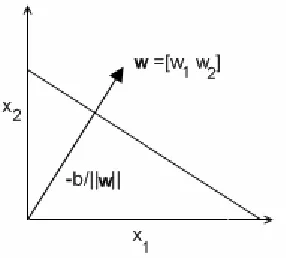
The neuron model described is nothing more than a biologically-inspired graphical representation of a simple, but powerful, mathematical function. This function, when set equal to 0, represents a hyperplane in an n-dimensional space and defines what is called a linear separator. The dimension in the case of the artificial neuron is the number of inputs plus one. For example, the equation for a neuron with two inputs is shown in equation 2.2.

(2.2) w₁x₁+w₂x₂+b=0

[image:11.612.234.377.554.683.2]

Given known weight and bias values, the graph of this function becomes a line (a two-dimensional hyperplane) with the normal w and offset -b/||w|| as shown in Fig. 2.2.

Since multiplying both sides of the equation by a nonzero value does not modify the orientation of the line, both sides are divided by the magnitude of the vector w,

normalizing the weight vector to obtain the same graph, but with updated labels. Fig. 2-3 shows the updated graph along with a new vector (dashed arrow) that is to be classified.

Figure 2-3: Linear Separator after normalizing the weight vector. The dotted line is an input vector that is to be classified.

The power of the linear separator lies in its ability to classify any given input x by

determining on which side of the hyperplane it sits. In the simple two-input example (Fig. 2-4) it can be shown that given any 2-dimensional input vector the output of the equation

b x−

wˆ is the perpendicular distance of the point from the line of the linear separator.

Figure 2-4: Classification of an input vector x.

The dot product between the input and weight vectors gives the magnitude of the

projection of the input vector onto the weight normal. Subtracting b (adding -b) results in a positive value if the vector projects past the line, and vice versa. By encapsulating the function by a sign function, any input can be classified as belonging to either the positive or the negative class. This two-dimensional example generalizes to any number of dimensions making it a powerful tool in various machine learning algorithms.

usefulness of the margin value will become clear in the following section in which learning methods are introduced.

2.5 Learning Algorithms

2.5.1

Single Layer Perceptron

The early artificial neuron was very capable but required that the weights were set

manually. Many simple systems, such as the digital AND, OR, and NOT gates were easily implemented. However, larger systems required quite a bit more work.

In 1957, Frank Rosenblatt, in his published book, “Principles of neurodynamics: Perceptrons and the theory of brain mechanisms” [3], introduced the Perceptron – a model based on the artificial neuron and including a learning algorithm which was the first big step in supervised training methods.

The algorithm for training a single neuron, in a slightly altered form, is shown in Listing 1.

Listing 1: Frank Rosenblatt’s Perceptron Learning Algorithm

This is an error-driven algorithm which modifies the weights in an effort to minimize misclassifications. The algorithm was proven to converge to a valid solution after a limited amount of iterations under the condition that the data are linearly separable (there exists a hyperplane that can fully divide the positive and negative set). In the case where the data is not linearly separable, the algorithm never terminates.

The choice of yixi as the weight increment is attributed to the gradient ascent function

optimization strategy. The gradient ascent method uses the derivative (gradient) of the function surface with respect to the optimization variable as a means to maximize the function output. Once the gradient of the function is calculated, a step is taken in that direction. The size of the step depends on the gradient slope. In this case the adjustment is made over many input-output pairs, and thus a small fraction of the gradient is actually taken repeatedly over multiple iterations. The gradient is recalculated at every iteration and the algorithm terminates once it becomes small enough (a relatively flat surface is reached).

Pick initial weight vector (including b), e.g.: [0 … 0] Repeat until all points correctly classified

Repeat for each Input

Calculate margin

i i

y w,x for point i If margin > 0, point is correctly classified Else

change weights to increase margin; change in weight proportional to y_ix_i

Recalling the significance of the margin, negative values represent those inputs which were misclassified. A large magnitude implies a big adjustment. It therefore makes sense to define the optimization problem as maximizing the margins for the misclassified points. Optimally, the sum of the margins becomes zero which implies perfect classification of the training set. The function to be optimized is therefore:

(2.3)

( )

=

∑

ied misclassif

,

i

i i

y

f w w x .

The gradient of this function with respect to the weights happens to be:

(2.4) ∇

( )

=

∑

ied misclassif i

i i

y

f w x

w .

Rosenblatt’s research coined the term Single Layer Perceptron in which there are one or more output neurons on the output layer and a multiple inputs on the input layer. Other networks that Rosenblatt experimented with were the cross-coupled Perceptron in which connections joined units of the same layer, and multilayer back-coupled perceptrons, which had feedback paths from units located near the output. While he did propose a back-propagating error method, no one could come up with a way for it to converge.

The discoveries made by Rosenblatt naturally brought new interest into the area of Neural Networks. Unfortunately, this interest dwindled in 1969 when Minksy and Papert published their book Perceptrons [4] in which they revealed their discoveries about the limitations of the applications of the Perceptron model. One elegant example used in their arguments was the basic XOR problem. This two input and one output system is linearly inseparable and cannot be learned using the Perceptron model. It is shown in Fig. 2-5.

Figure 2-5: Input vectors for the XOR problem

the XOR problem space is shown in Fig. 2-6. The addition of the hidden layer is

equivalent to creating linear separators of linear separators. In other words, the output of two decision boundaries (at the hidden layer), is used as input to the final linear separator.

Figure 2-6: A Multilayer solution to the XOR problem

The resulting outputs for each of the possible inputs are:

x1 x2 o1 o2 y

0 0 0 0 0 0 1 0 1 1 1 0 0 1 1 1 1 1 1 0

Figure 2-7: Outputs of each of the linear separators for each input combination

The hidden layer and its weights define two linear separators (Fig. 2-8a). The outputs of these separators are processed by the linear separator of the output neuron (Fig. 2-8b).

While their introduction of a hidden layer was an important step, Minksy and Papert’s other, rather pessimistic, discoveries were enough to cause widespread decline of further research into the subject.

2.5.2

The Multilayer Perceptron

In 1974, Paul Werbos presented a method for weight adjustment in the hidden layers during a dissertation at Harvard University [5]. Unfortunately, his work went largely unnoticed. It wasn’t until 1986 when Rumelhart, Hinton, and Williams published “Learning Internal Representations by Error Propagation” [6] in which they proposed a modified Multilayer Neural Network along with a training algorithm for adjusting

weights connected into the hidden layers. Their work was independent to that of Werbos, but they are often credited with the discovery.

The biggest addition in Rumelhart’s, Hinton’s, and Williams’ model is the incorporation of a differentiable activation (or transfer) function. This simple modification allowed them to use an existing mathematical tool called the generalized delta rule (also known as the heavy ball method in literature [7] [8] [9]) which is related to gradient ascent. The technique was termed Backpropagation in the context of the neural network and remains the most popular method for weight adaptation in the hidden layers. It functions similarly to Rosenblatt’s method, but it minimizes the misclassification error rather than

maximizing the margin of misclassified training pairs. The ability to adjust weights in the hidden layers opened up new possibilities such as the training of linearly inseparable data. With the birth of the Multi Layer Perceptron, interest in the field of neural networks rekindled.

The key to the Backpropagation algorithm is the differentiability of the activation function which implies smooth changes to the output values due to a small weight changes in the network. The optimization function at the output is defined to be the training error over all training vectors:

(2.5)

∑

(

(

)

)

=

−

=

T i i i

d

y

E

0 2

,

2

1

w

x

in which y(xi, w) is the network output given the ith input vector, diis the expected output,

and T is the number of training vectors. It is clear that since y(xi, w) is smooth and dii is constant, the error function is smooth as well. To utilize gradient descent, the gradient of this function is necessary (Eq. 2.6).

(2.6)

∑

[

(

(

)

)

(

)

]

= ∇ − = ∇ T i i w i i

wE y d y

0

,

,w x w

x

The gradient for the output with respect to the weights is obtained by applying the chain rule of differentiation as shown in Eq. 2.7 and Fig. 2-9.

(2.7)

Figure 2-9: Calculating the output gradient with respect to the weights.

The derivative is broken down into a product of the derivative of the output with respect to the activation value (the slope of the activation function with the current value z) and the derivative of the activation value with respect to the current weights (for a Single Layer Perceptron, this value is simply the current input x). By the rule of gradient descent, for every neuron at the output layer, the weight vector should be updated by an element-by-element product of the output error vector and the activation function gradient at that activation value.

(2.8)

(

) ( )

i i i w x z z F d y w w E ∂ ∂ − − ← ∇ − ← η η w w

The parameter η is a small value known as the learning rate. If a hidden layer is

introduced, which includes its own set of weights, a method is required for obtaining the gradient of the output y with respect to one of the hidden layer weights. The same

procedure is used, but since the input into the output layer is an output from the hidden, a recursive loop is observed as shown in Eq. 2.9 and accompanying Fig. 2-10.

( )

(2.9)

( )

( )

( )

        ∂ ∂       ∂ ∂ →         ∂ ∂       ∂ ∂ =         ∂ ∂       ∂ ∂ =        _∂       ∂ ∂ = ∂ ∂ ij i i ij i i ij ij ij w y w z z F w y w z z F w z z z F w z z y w y

Figure 2-10: Chain rule for the output gradient with respect to the weights.

In more general networks, multiple weights near the input may affect the signal coming into a neuron on a further layer. In such cases, the gradient of the signal can be obtained by summing the effects over all possible paths.

The intuition is built on the observation that the output gradient is a function of the signal on each of the inputs into the output neuron. Changing a weight on a hidden layer of some hidden neuron produces a gradient on the signal between the hidden neuron and the output neuron. Assuming that there is only one hidden layer as in most networks, the gradient on any of the signals is calculated using the base case above.

In order to implement Backpropagation a new quantity δ is introduced. At the output layer, the delta for a single neuron is:

(2.10)

(

) ( )

z z F d y z E ∂ ∂ − = ∂ ∂ = δ .

To obtain the deltas for the jth neuron in the hidden layer l, the deltas from the (l+1)th layer are propagated backward and multiplied by the derivative of the activation function acting on the input of the neuron:

(2.11)

( )

jk

L k l k l j l j l j w z z F l

∑

+ = + ∂ ∂ = 1 0 1

δ

δ

.

By substituting Eq. 2.10 into the general case of Eq. 2.8, the weight connecting neuron i from layer l to neuron j in layer l+1 is updated by:

The name Backpropagation comes from the way in which the δ value is propagated backwards through the network. Reusing the deltas as they are propagated back is the grounds for its efficiency. Listing 2 summarizes the Backpropagation algorithm.

Listing 2: Backpropagation Summary

2.6 Training the Multi Layer Perceptron

This section summarizes some of the issues that plague MLP training as well as some of the parameters and modifications to the training algorithm that the implementer has control over. One of the major drawbacks of training the MLP is the lack of automated training parameter discovery. The implementer is forced to experiment with such things as numbers of layers, layer sizes, learning rates, methods of learning, convergence conditions, length of training, etc. The decisions made are mostly based on heuristics and experience. Options exist that may simplify this process, but usually involve tradeoffs and never completely eradicate the problem.

Several issues due to improper setup as well as those inherent in the MLP are presented, along with methods that aim to reduce them. As will become evident, many design choices are influenced by what is desired and how much time and resources are available.

2.6.1

Combination Functions

The combination function defines the transformation of the two vectors (w,x) to scalar (z) in the first neuron processing step. The MLP, in nearly all cases, uses the dot-product. However, other networks exist – most popular being the Radial Basis Function network in which, as the name implies, the RBF function is used instead [10].

2.6.2

Activation Functions

As discussed in the previous section, the activation function is utilized in the second step of the neuron’s forward process and its derivative is utilized during Backpropagation. The activation function in the hidden layer needs to be nonlinear for the network to be capable of learning from datasets that may not be linearly separable. Activation functions that produce values centered around zero (i.e.: [-1.0,1.0]) are usually preferred as they generally converge quicker due to improved numerical conditioning [11]. The two most popular activation functions are the sigmoid and hyperbolic tangent. Table 1 shows these two functions as well as an approximated version (used in this work) [12].

Initialize weights to small random values

Repeat until error over entire training set is small enough Repeat for all Training input-output pairs

Propagate forward by computing the outputs of each layer in succession

Compute δ at the output layer

Propagate the δ value backward through the layers

Updating the weights on each layer Loop

( )

z

F

( )

z z F ∂ ∂ Sigmoid z e− + 1

1 F

( )

z

(

1−F

( )

z

)

Hyperbolic Tangent

( )

_zz _zz

e e e e z ₋ − + − =

tanh

( )

( )

2 2 1 tanh 1 z F z − = − Hyperbolic Tangent

(LeCun’s Appx..) 

     = z 3 2 tanh 7159 .

1

(

1.7159 ( )

)(

1.7159 ( )

)

7159 . 1 1 3 2 z F z F − +            

Table 1: Activation Functions

The popularity of these activation functions is attributed to the ease of obtaining the derivative using values already in memory. The graph of each is shown in Fig. 2.11.

Figure 2-11: Activation function curves

2.6.3

Bias Term

As described in the previous section, each neuron in the MLP model contains a bias term that shifts the linear separator’s hyperplane along the weight normal. In many

implementations of neural networks, the bias is represented simply as another weighted input with the constant value of +1 or -1 (neither have an advantage when training). The corresponding weight is trained just like any other on that neuron. The bias term is optional, although the theory of the universal approximation does not hold without it [13]. One way in which the bias may be avoided is by forcing the condition that the outputs on any layer sum to a nonzero constant [14]. This is most easily done by preprocessing the input data so that each vector has elements which sum to the same constant value.

The neuron processing equation, with the bias term treated as a weighted input is

(2.13)

(

)

_

     =

∑

+ = − − 1 0 1 , 1 * n L l l n j l n j

n F w x

in which L j n

n

w −1+1, _{is the weight associated with the bias term. This simplified equation will}

make the implementation much simpler as will be seen in Chapter 6.

2.6.4

Initial Weights

The choice for initial weight values is quite important when initializing the network since it decides the initial position in the search space. Values should be small enough so to prevent the neuron outputs from saturating. Recall that the slope of the activation function becomes flat at the input extremes. Because weight updates are proportional to this slope, learning may become extremely sluggish. A good choice of weights, therefore, is one that produces midrange function signals. A good practice is to select zero centered random weights within a small range.

2.6.5

Local Minima

One of the major issues that plague MLP training is the possibility of the gradient descent method to become trapped in a local minimum. This is a direct result of the fact that the error surface that is being searched is non-convex. The strategies described in the following sections may help in this matter.

2.6.5.1

Learning Rate

An important parameter that needs to be selected if performing incremental learning (in which weights are updated after every training pair) is the learning rateη. The purpose of this parameter is to subdue the effect of the gradient descent on the values of the weights. Every application of the gradient descent method is valid only locally for the input-output pair currently applied. Too big of a change would likely negatively affect the accuracy on the remaining set. Values are typically in the range of (0, 1].

The learning rate value should be selected based on, among other things, the number and size of the layers and the number of training vectors. Too high of a value can cause chaotic oscillations around the solution. Values too low may cause a very long training time.

One option is to implement a dynamic learning rate that uses information about the conversion progress to adapt the learning rate. There is a good amount of research on the topic. However, a simple and effective method is to decrease the learning rate

periodically over time. This practice also guarantees convergence.

2.6.5.2

Momentum Term

the search overcome any minimums encountered along the general downward slope of the gradient. The updated weight updating step, utilizing the deltas of the previous weight updates is:

(2.14)

t t t

t i

w

t E

w w w

w w

∆ + ←

∆ + ∇ − = ∆

+

−

1

1

α

η

.

Note the addition of the momentum term

α

which needs to be selected. The effect of the change is that sequential weight changes in the same direction accelerate, while those of opposite signs cause the changes to decelerate, as expected.

2.6.5.3

Multiple Training Sessions

Another, simple and brute force, method to improve the chance of finding the global minimum is to train on the same data modifying only the initial weight values. Of course, this method can significantly increase the learning time and has no guarantees.

2.6.6

Incremental vs. Batch Learning

Weight updates may be performed after the calculation of the error of each individual input-output sample or at the end of a full epoch. The former case is called incremental learning (also instantaneous or pattern learning). In this mode, the delta is propagated back as described in the previous section, and the weights are updated following the Backpropagation of each training vector’s output error. It is important that the deltas are “pushed” onto the neurons of the previous layer before modifying the weights themselves on any particular layer so that the error “blame” is placed on the neurons for which the connections were strongest during the forward propagation.

When performing incremental training, a recommended strategy is to present the network with the training samples in random order within the epoch. This prevents the network from giving the early samples in the set a greater priority and may reduce the risk of getting stuck in a local minimum.

In batch learning mode (also epoch learning), the samples from the entire training set are propagated forward and back through the network accumulating all the weight

adjustments for each layer. Training samples do not need to be applied randomly as this would make no difference in the final values. The asynchronous nature between iterations of one epoch makes batch learning a better candidate for parallel implementations. The greatest benefit to batch learning, however, is the possibility of applying adaptive learning methods that are described next.

2.6.6.1

Adaptive Learning Techniques

Standard BP uses the derivative of the activation function as a part of the weight updating calculation. Due to the shallow slope at high magnitude input values, the change in weight may be very small for large error values. RPROP, on the other hand, uses only the sign of the dE/dw value along with an externally defined value to update the weights. The weight change is calculated as shown in Eq. 2.15.

(2.15)          < ∂ ∂ ∆ + > ∂ ∂ ∆ − = else , 0 0 if , 0 if , ij t ij ij t ij t ij w E w E w

The adaptive feature of the RPROP algorithm comes from the self-adjustment of the weight delta values as follows:

(2.16)            ∆ <         ∂ ∂         ∂ ∂ ∆ >         ∂ ∂         ∂ ∂ ∆ = ∆ − − − − − − + else , 0 if , 0 if , 1 1 1 1 1 t ij t ij t ij t ij t ij t ij t ij t ij w E w E w E w E

η

η

in which 0<

η

− <1<

η

+. In words, if the slope of the error curve with respect to some weight negated, this signifies an overshoot and the multiplier for that weight is decreased. In this situation, the weight is not modified at this epoch. If the slope direction remained the same, the conversion can be accelerated by increasing the multiplier for that weight. Some parameters that can be modified are the values of

η

+ _and

η

−_{, and the maximum} and minimum of the deltas.

The Quickprop (or Qprop) algorithm is a secant method which uses the property that the gradient of the error surface with respect to the weights is zero at all local minima. One way to obtain the optimal weight values is to solve the following system of equations:

(2.17)

(

)

(

)

(

, ,...,

)

0

... 0 ,..., , 0 ,..., , 1 0 1 0 2 1 0 1 = ∂ = ∂ = ∂ n n n n w w w E w w w E w w w E

(2.18)

( )

( )

( )

t i t i t i t i t i i t i t

i E w

w w w E w E w w ∂       − ∂ − ∂ − = − − − + 1 1 1 1

η

.

2.6.7

Generalization and Overfitting

2.6.7.1

Definition

The typical purpose of a neural network is to be accurate not only on the training set, but any new novel input from the same population. A network capable of classifying many novel inputs correctly has a good generalizing characteristic. Training a network so that it retains high generalizing capability is not easy. There is much research in this area that is beyond the scope of this thesis. The following are just several recommendations that should be followed when choosing the training data [14]:

1. The choice for attributes in the input data must make sense with that of the output class. In other words, there needs to be some correlation, even if theoretical, between the cause and effect.

2. For the case of continuous functions, the function that is being learned should be smooth. While this is not a necessity, it is beneficial for the Backpropagation algorithm which relies on the gradient of the function as a choice for weight updates. In some cases, a preprocessing of the input data, such as by using Principal Component Analysis, can help.

3. The training set should be sufficiently large and be a good representation of the data that the neural network is expected to come across. A good representation is defined as input samples that cover a large part of the input space and are evenly separated.

Following these rules requires some prior knowledge of the function being approximated.

Generalization can be lost if the training algorithm is run for too long on the training data. In this phenomenon, known as overfitting, the surface of the hypothesis function, in an effort to “touch” every point in the training set, may become jagged having many irregularities between the training points. This in turn leads to the loss of interpolating ability and lack of generalization. It is therefore necessary to prematurely stop the training process before it enters the overfitting stage. This is difficult, if not impossible, to achieve if using only the errors in the training set as the criteria for the stopping condition.

2.6.7.2

Cross-Validation and Early Stopping

model parameters (such as network size), or for determining when to stop training (early stopping).

Various partitioning schemes exist based on the cross-validation technique. In the simplest method, called Holdout Validation, the initial training data is split into the two aforementioned sets. The training data is used to train the model. After each iteration of the training set the validation set is used to compute the accuracy. Fig. 2-11 shows typical behavior of the errors on the training and validation sets as a function of the iteration number. Early stopping often incorporates the holdout validation scheme. The point at which the algorithm should stop is marked by a vertical dotted line. Note that the error on the training set continues to decrease.

Figure 2-12: Training Set error and Validation Set error as a function of training iteration number.

A more advanced partitioning scheme, known as K-Fold cross-validation, entails partitioning the original set into k subsets. The same algorithm is run k times by leaving one of the k subsets out and using it as the validation set. The results from the k runs are accumulated and processed (often by taking an average). While it is not obvious how to use this partitioning scheme for early stopping, it can be used to evaluate the network structure for generalization.

A third partitioning scheme, known as Leave-one-out cross-validation, is simply K-Fold cross-validation with k set to the number of training samples. In other words, the network is trained k times, reserving only one of the training samples for validation. As expected, this method takes a very long time and is more applicable to smaller problems.

2.6.8

Jitter

This simple, but powerful method works on the principle that input vectors that are close together should produce outputs that are close together. The method involves modifying the input vectors by changing their continuous attribute values in very small percentages. This can also be effective when the training set available is quite small and works

2.6.9

Weight Decay

Large weights in an MLP are known to negatively affect generalization performance. Having large weights at the hidden layer can easily cause the hypothesis function to become rough with small changes in the input and have near discontinuities. Large weights leading into the output layer can cause the output to become too large and leave the range of the possible outputs. Weight Decay is a method in which the error function is augmented with a weight penalty term. An example of a penalty term is a fraction of the squared sum of the weights (Eq. 2.19). This simple addition forces the network to try and keep down the weight values and prevents these kinds of problems.

(2.19) =

∑

(

(

)

−

)

+

∑

= k

k T

i

i

i d w

y E

0

2

, 2

1

w x

in which k is the set of indices for all the weight parameters.

2.7 Network Architecture

The most obvious and arguably most critical parameter that the implementer has control over is the number of neurons in the hidden layer, or whether to include a hidden layer at all. Naturally, choosing to forego the hidden layer would speed up the learning process considerably. In contrast, there are rare cases in which there is a need for multiple hidden layers. The size of the input layer is set by the dimension of the input data as is the output layer due to the output data. The hidden layer, however, is under full control. Selecting a proper number of units in the hidden layer(s) takes into consideration the dimension of the inputs and outputs, size of the training set, complexity of the function to be learned, number of layers and network architecture, type of activation function used, training algorithm, and other factors. Often, the best action is to simply train multiple networks and see which one works best.

As part of an effort to automate the task of choosing the network architecture, new mechanisms which dynamically adapt the number of neurons as well as connections between them have been developed. These generally fall into constructive and pruning algorithms in which neurons are added or removed automatically as the learning

progresses. These techniques are beyond the scope of this work. A summary of popular constructive algorithms is presented in [18], [19] and [20]. Pruning algorithms are summarized in [21] and [20].

2.8 Convolutional Networks

The standard Multi-Layer Perceptron model consists of two or more layers of neurons. Each layer is usually fully-connected to the layer before it, meaning that every neuron on layer l is connected to every neuron on layer l-1.

Traditionally, when applying neural networks to 2-d inputs, such as images, so called feature extractors are placed between the raw image input and the input layer of the network. These feature extractors, or kernels, are hand tuned to extract information such as edges and discard irrelevant variables. The process is called convolution.

LeCun et al. [22] [23] have tried to remove this extra step of needing to manually create the kernels. Instead, their design, known as the Convolutional network, uses

Backpropagation to automatically train the feature extractors.

Convolution networks (consisting of convolution and subsampling layers) are similar to fully-connected networks (consisting of fully-connected layers), and can in fact be interconnected with convolution layers appearing before fully-connected layers in the network. Convolutional layers borrow the idea of an image feature extractor (or kernel) from image processing and train these kernels automatically (just as fully-connected layers train the weights going into them).

Figure 2-13: Convolution Layer network architecture.

The main advantage to Convolutional layers in comparison to standard layers, however, is their inherent invariance to image transformations such as shifts, scales, and rotates. A standard layer, upon learning from a training set of shapes, for example, would result in having similar weights repeated at certain intervals. On the other hand, the Convolutional layer kernel which is made of a relatively small set of weights traverses the entire image. This shared weight concept is not new, but is found to work well for 2-dimensional inputs. An example of LeCun’s networks is shown in Fig. 2-13. It is the LeNet-5 [12] which was designed to recognize handwritten characters.

Figure 2-14: LeNet-5 Network

Note that the LeNet-5 architecture consists of convolution layers, which function as described above, and subsampling layers, which take averages of closely spaced pixels to produce a smaller feature map. Subsampling helps reduce the effect of shifts of the input image between training samples. The implementation in this work achieves a similar effect by combining the convolution and subsampling layers into one by moving the nxn kernel two pixels at a time in the x and y directions.

2.9 Related Work

Being a relatively easily parallelizable algorithm, the standard MLP algorithm (consisting of only fully-connected layers) has been parallelized on a vast number of devices,

Chapter 3: Support Vector Machines

3.1 Chapter Introduction

Support Vector Machines (SVMs) are similar to the Multi-Layer Perceptron (MLP) in that they generalize into the family of linear classifiers, or separators, introduced in the previous chapter. The methodology for training, however, is quite different. While MLPs are largely based on heuristics (even the very first neuron model was based on heuristics), SVMs borrow proven theorems and tools from the fields of optimization theory,

generalization theory, and statistical learning theory making them more understood. SVMs, as will be revealed, hold many important advantages compared to other training methods such as the MLP. The chapter discusses early motivation for this learning system and introduces some of the concepts which serve as the foundations for its functionality.

3.2 Background

It is difficult to pinpoint the exact point in history at which Support Vector Machines appeared, but much of its advancement is credited to Vladimir Vapnik who is considered by many to be the main inventor and contributor. It has been widely accepted that the beginnings of SVMs appeared with the publishing of the book “Estimation of

Dependencies Based on Empirical Data” (1979) [28] in which Vapnik provided the foundations of statistical learning theory. The SVM algorithm itself was introduced in [29]. The main purpose of the SVM was to overcome some of the shortcomings of existing classifiers – especially those of the MLP. Both the SVM and the MLP belong in the class of linear learning machines that were introduced in the previous chapter but are very different in the techniques that they employ. This difference is largely attributed to the dissimilar processes by which the two came about. SVMs were designed using existing proven theories and concepts taken from optimization theory, generalization theory, statistical learning theory, etc. The MLP takes concepts from existing theories as well, but it is also largely based on heuristic models such as the very first McCulloch and Pitts neuron model itself (which in some way was based on the yet little understood neuron inside the brain).

3.3 Training

model that really set the two apart. Also, unlike the MLP, the SVM is inherently only capable of distinguishing between two classes, making it a binary classifier. For the purpose of this chapter, elements are either classified as either positive (+) or negative (-).

Like the MLP, the goal of SVM training is to produce a linear n-1 dimensional

hyperplane in an n-dimensional input space that separates the two classes. The SVM is known as a maximal-margin classifier because it attempts to find a hyperplane that not only classifies each training vector correctly, but it optimizes its position and orientation by taking into account the perpendicular distances of the closest points to the hyperplane. In other words, the algorithm attempts to find the widest possible “street” (of widest margin) that can still classify all training vectors. This constraint can be relaxed, as will be explained later. The name “support vectors” comes from the algorithm’s objective to discard any vectors that do not affect the margin; those that do not touch the edges of the “street.” A toy example of a linearly separable two-dimensional problem is shown in Fig. 3.1 with the support vectors circled in red.

Figure 3-1: A toy example of a widest-margin classifier in two dimensions.

3.3.1

Linearly Separable Case

The SVM can be applied to many real problems. However, for the purpose of this

section, the theory is first introduced in the simplest case in which all training vectors are linearly separable. Once the main concept is introduced, further modifications will be described that extend the SVMs application to more realistic cases.

As a review, the hyperplane of a linear learning machine is defined by the function:

(3.1) f x w x b or f x b

d

k k

k + = ⋅ +

=

∑

=

w x

) ( )

(

1

training vector and d− be the distance to the closest negatively classified training vector, maximizing the margin implies maximizingd₊ +d₋. For the purposes of optimization, the goal is to find a representation of the margin width in term of the optimization

variables w and/or b. It is a known property of linear classifiers that scaling the values w, b by the same positive factor does not change the function. On the other hand, the values of d+ and d− will be impacted. For derivation purposes, d+ and d− can be forced to 1, resulting in the following two inequalities:

(3.2)

{

}

{

| 1

}

1 ) ( 1 | 1 ) ( − = − ≤ + ⋅ + = + ≥ + ⋅ i i i i y i b b y i b a w x w x

which can be combined into one convenient expression of Eq. 3.3.

(3.3) y_i

(

x_i ⋅w +b

)

−1≥0 ∀i

Assume that there exist points for which the equality in Eq. 3.2a holds and another set of points for which the equality in Eq. 3.2b holds (this implies a trained w and b). The points satisfying Eq. 3.2a lie on the hyperplane xi ⋅w +b=1 which has a perpendicular

distance from the origin of 1−b w . Similarly, those satisfying Eq. 3.2b lie on the hyperplane xi ⋅w +b=−1 which has a perpendicular distance from the origin of

w b

−

−1 . These points are known as the support vectors as they touch the extremities of the margin. All other points (satisfying the inequality of Eq. 3.2a and 3.2b) are non-support vectors and would not change the final values of w and b should they be removed.

Since both hyperplanes are parallel, the distance, m, between them is obtained by taking the difference between their perpendicular distances from the origin.

(3.4)

(

) (

)

w w b w b m 2 1 1 = − − − − =

Maximizing the hyperplane, therefore, amounts to minimizing w2 2.

The problem can be reformulated into Lagrangian form as shown in Eq. 3.5. By doing so the constraint in Eq. 3.2 is replaced with constraints of Lagrange multipliers

α

_i,i=1,...,l (one for each of the l input training vectors) which are easier to handle. Also, the training data will appear during the training and classification phases in the form of dot products – a property that is central to the SVM’s ability to generalize to the nonlinear case as will be shown in later sections. The primary Lagrangian is

(3.5)

∑

(

)

∑

= = + + ⋅ − ≡ l i i l i i i i

P w y b

L 1 1 2 2 1 α

Because the objective function itself is convex and those points which satisfy the

constraints are convex, the problem becomes a quadratic programming problem. With the help of optimization theory, the problem can be reformulated once again into a dual form which is known as the Wolfe dual [30]. The dual formulation is often easier to solve due to the difficulty in handling inequality constraints. The procedure for transforming a primal into a dual is to zero the derivatives of the primal function with respect to the optimization variables, and substitute the resulting relations into the primal. This process removes the dependence on these variables. For the primal obtained above, the process is as follows.

Differentiating the primal form with respect to w and b and setting it to zero gives:

(3.6)

(

)

(

, ,

)

₀

0 , , 1 1 = = ∂ ∂ = ⇒ = − = ∂ ∂

∑

∑

∑

= ∈ = l i i i P l i i i i l i i i i P y b b L y y b L α α α α α w x w x w w w .

Substituting back into the primal results in the dual problem:

(3.7)

(

)

[

(

)

]

∑

∑

∑

∑

∑

= = = = = ⋅ − = + ⋅ = − + ⋅ − ⋅ ≡ ) , ( ) 1 , 1 ( ) , ( 1 1 ) , ( ) 1 , 1 ( ) , ( 1 2 1 2 1 1 2 1 l l j i j i j i j i l i i l i i l l j i j i j i j i l i i i i D y y y y b y L x x x x w x w w

α

α

α

α

α

α

α

.

The constraints for this problem, borrowed from the primal version, are:

(3.8) 0 , 0 1 = ∈ ≥

∑

= l i i i i y l i

α

α

.

The Wolfe dual maximum occurs at the same point of w, b and

α

i as the primal

Lagrangian’s minimum subject to the two problems’ corresponding constraints. The values of

α

i at the solution are greater than zero for those training vectors which lie on

The Karush-Kuhn-Tucker (KKT) conditions, also borrowed from the field of nonlinear programming techniques, are conditions that if satisfied, are necessary and sufficient for optimality. For the case of the primal problem, they are:

(3.9)

(

)

(

)

[

y b

]

i

i l i b y y b L d v x y w w L i i i i i i l i i i P l i iv i i v v P ∀ = − + ⋅ ∀ ≥ = ≥ − + ⋅ = = ∂ ∂ = = − = ∂ ∂

∑

∑

= = , 0 1 , 0 ,..., 1 , 0 1 0 ,..., 1 , 0 1 1 w x w x

α

α

α

α

Once the

α

i’s are found, w is obtained directly from one of the primal constraints:

(3.10)

∑

= = l i i i i y 1 x w

α

Once w is calculated, b can be obtained. Since the b does not appear in the dual problem, a safe way to obtain it is to use the mean of the solutions of the “complimentarity” KKT condition:

(3.11)

α

i

[

yi

(

xi⋅w +b

)

−1

]

=0

for i’s corresponding to non-zero Lagrange multipliers (

α

i >0). Another method is to solve the following:

(3.12)

(

)

(

)

2 max

maxy_{i 1} i y_{i 1} i

b=− =− w⋅x + =+ w⋅x

Classifying a novel vector becomes a simple matter of calculating:

(3.13) f(x)=sgn

(

w⋅x+b

)

3.3.2

Non-separable Case

Up to now, it was assumed that the training vectors are linearly separable. This

assumption rarely holds in real world problems. Thankfully, there is a solution that was provided by Cortes & Vapnik in 1995 [31]. By introducing slack variables, the

constraints given in Eq. 3.2 can be relaxed. The new constraints are as follows:

The goal is to keep slack variables as small as possible. A value greater than one implies a misclassification. The sum of slack variables is, therefore, an upper bound on the number of classification errors. The original objective function w 2 2is augmented with the penalty factor for the slack variables as follows to form

(3.15)       +

∑

= l i i C w 1 2

2

ξ

.

where C is user modifiable. Higher values of C put a higher penalty on misclassifications. The derivation of the dual Lagrange problem is similar to that above. Details can be found in [32]. The new dual optimization problem becomes:

(3.16)

∑

∑

= = ⋅ − ≡ ) , ( ) 1 , 1 ( ) , ( 1 2

1 ll j i j i j i j i l i i

D yy

L

α

α

α

x x

With the constraints:

(3.17) 0 , 0 1 = ∀ ≤ ≤

∑

= l i i i i y i C

α

α

The only difference is an upper bound on the

α

_i’s making it into a box-constrained problem. Note that the slack variables disappear. For reference, the new primal Lagrangian is:

(3.18)

∑

∑

[

(

)

]

∑

= = = − + − + ⋅ − + ≡ l i i i l i i i i i l i i

P w y b

L 1 1 1 2 1 2 1

ξ

µ

ξ

α

ξ

x w

in which the

µ

i’s are new Lagrange multipliers introduced to enforce positivity of the

i

ξ

’s.

(3.19)

(

)

(

)

[

]

i i b y i i i l i b y i C L y b L d v x y w w L i i i i i i i i i i i i i i P l i i i P l i iv i i v v P ∀ = ∀ = + − + ⋅ ∀ ≥ ∀ ≥ ∀ ≥ = ≥ − + ⋅ ∀ = − − = ∂ ∂ = = ∂ ∂ = = − = ∂ ∂

∑

∑

= = , 0 , 0 1 , 0 , 0 , 0 ,..., 1 , 0 1 , 0 0 ,..., 1 , 0 1 1

ξ

µ

ξ

α

µ

α

ξ

µ

α

ξ

α

α

w x w x

The higher complexity of the primal Lagrangian with the addition of slack variables further validates the preference for solving the simpler Wolfe dual problem. From this point on, only the dual formulation will be considered.

3.3.3

Non-linear Case

The Wolfe dual can be rewritten to conform to the representation of a linearly constrained quadratic programming problem:

(3.20)

( )

α

α

α

α

α

α

α

ψ

T T n i i T c G G − = − =

∑

= 2 1 2 1 1

in which c is a vector of all -1’s. The problem solution is subject to conditions:

(3.21) 0 ,..., 1 , 0 1 = = ≤ ≤

∑

= i n i i i y n i C

α

α

in which G takes on the values ai,j=yiyjxi,xj.

In order to extend the application of SVMs to nonlinear problems, [29] applied an old kernel technique, known as kernel-induced spaces, in which they replaced the values of the matrix G with ai,j = yiyjK

(

xi,xj

)

. In effect, they replaced dot product operations with

Polynomial (homogeneous)

(

)

d

K a,b = a⋅b

Polynomial (inhomogeneous)

(

)

(

)

d

K a,b = a⋅b +1

Radial Basis Function

(

)

(

2

)

exp

,b a b

a = −γ −

K , for γ >0.

Gaussian Radial Basis Function

(

)

_       ₋ − = ₂ 2 2 exp ,

σ

b a b a K Sigmoid

(

)

(

c

)

K a,b =tanh

κ

a⋅b + , for at least one κ >0and c<0.

The kernel operation is simplified before implementation whenever possible. For example, in the case of the inhomogeneous polynomial kernel:

(3.22)

(

)

(

)

(

)( )

∑

(

)(

)

∑

∑

∑∑

∑

∑

= = = = = = = + + = + + =         +       + = + ⋅ = n i i i l l j i j i j i n i i i l i l j j i j i n j j j l i i i c cb ca b b a a c b a c b b a a c b a c b a c z x K 1 2 ) , ( ) 1 , 1 ( ) , ( 1 2 1 1 1 1 2 2 2 2

, a b

Since only the kernel matrix is affected by the input vectors, the kernel function

decouples the data from the problem. The quadratic program problem is solved in exactly the same way, but with a different, usually larger kernel. More often than not, mapping the input vectors using the nonlinear kernel makes them linearly separable in the induced feature space. The classification step is modified in the same way – with dot products replaced by kernel operations.

3.4 Implementations

ramifications of this discovery were significant in that it was possible to apply existing well-developed solvers.

Unfortunately, existing solvers act on the assumption that the entire kernel matrix is in fast memory (usually RAM) at all times. The size of this matrix in the context of SVMs grows quadratically with the number of input training vectors. With number of training vectors in the hundreds of thousands being not uncommon, the memory requirement for the training from such datasets becomes too large. Even with the rapid increase in memory capacity in modern hardware, the poor scalability to increased training set sizes called for new, memory efficient methods. Two such methods which gained wide acceptance are the Working Set technique (e.g.: Chunking and Decomposition) and the

Sequential Minimal Optimization technique.

3.4.1

Working Sets

The main concern, as expressed above, is the lack of memory for the kernel matrix due to the large size of training sets. The working set technique, introduced by Osuna [],

attempts to remedy this issue by working on a relatively small subset of the training set at a time. The generalized pseudo-code is shown in Listing 3.

Listing 3: Generic Working Set Pseudocode

Initially, the subset of size N is chosen arbitrarily, usually randomly and evenly

distributed. The quadratic programming solver is put