Literature Survey on Various Classification
Algorithms in Machine Learning
Tanushree Dholpuria1Dr. Yuvraj Rana2
1
M-Tech Scholar 2ProfesssorRITS, Bhopal
Abstract: Machine learning is one of the fastest emerging technologies in the field of computing. It enables computers to lean without being explicitly programmed. In this paper, we present and discuss a various classification algorithm that can be used to predict Box-Office performance based on twitter messages. These algorithms can be applied to solve other problems as well, including- classifying ham or spam messages from the email dataset, classifying positive or negative reviews and many more. The focus of this paper will be mainly on Naïve Bayes, SVM, k-NN, Neural Network and Random Forest.
Keywords: Naïve bayes, SVM, k-NN, neural network
I. INTRODUCTION
Bigdata analytics is used to analyze the data from big data. This is actually the process of finding the hidden information /patterns from the repositories(Tsai, Lai, Chao, & Vasilakos, 2015). In machine learning we use a variety of analysis tool to determine the relationship between data from Big data. Machine learning basically uses statistic measure for analysis purpose(Mitchell, 2011). Our goal is to extract information from big data and transform into a human understandable format. In machine learning, classification, regression and clustering are three approaches in which instances are grouped into identified classes. Classification is a popular task in data mining especially in knowledge discovery and future plan, it provides the intelligent decision making, classification is not only used to study and examine the existing sample data but also predicts the future behavior to that sample data. The classification includes two phases. The first phase is learning process phase in which the training data is analyzed, then the rules and patterns are created. The second phase tests the data and archives the accuracy of classification patterns. Clustering approach is based on unsupervised learning because there are no predefined classes. In this approach data may be grouped together as a cluster(Tan, Steinbach, & Kumar, 2005). Regression is used to map data item into a really valuable prediction variable. In Classification technique various algorithms such as decision tree, nearest neighbor, genetic algorithm support vector machine (SVM) etc.(Pradhan, 2012). Machine learning is one of the fastest emerging technologies in the field of computing. It enables computers to lean without being explicitly programmed. In this paper, we present and discuss a various classification algorithm that can be used to predict Box-Office performance based on twitter messages. These algorithms can be applied to solve other problems as well, including- classifying ham or spam messages from the email dataset, classifying positive or negative reviews and many. Broadly machine learning are classified into two categories on the basis of signals or feedback.
1) Supervised learning: for example in computer if teacher give some input and need some outputs. So mainly our goal is to maps inputs to outputs. As an exception some input signals are partially available or restricted to special feedback.
2) Unsupervised learning: discovering hidden patterns in data. As no labels are assigns to learning algorithms and leave to finds its own outputs. Machine learning can also be categorized as classification, destiny estimation, clustering, reduction,
dimensionality etc. There are certain approaches of machine learning which are Bayesian Networks, Support Vector Machines, Artificial Neural Networks, Learning classifier systematic. In this paper, we examine the various classification algorithms and compare them.
A. A Probabilistic Approach
B. Naïve Bayes
Naive Bayes, also known as Naive Bayes Classifiers are classifiers with the assumption that features are statistically independent of one another(Vadivukarassi, Puviarasan, & Aruna, 2017). Unlike many other classifiers which assume that, for a given class, there will be some correlation between features, naive Bayes explicitly models the features as conditionally independent given the class. This provides all over simplistic restriction on the data in practice this classifier which is competitive with more sophisticated techniques and enjoys some theoretical support for its efficiency. Because of the independence assumption, naive Bayes classifiers are highly scalable and can quickly learn to use high dimensional features with limited training data. This is useful for many real world datasets where the amount of data is small in comparison with the number of features for each individual piece of data, such as speech, text, and image data. Examples of modern applications include spam filtering, automatic medical diagnoses, medical image processing, and vocal emotion recognition. This classification technique is based on Bayes’ Theorem with an assumption of independence among predictors. In simple terms, a Naive Bayes classifier assumes that the presence of a particular feature in a class is unrelated to the presence of any other feature. For example, a fruit may be considered to be an apple if it is red, round, and about 3 inches in diameter. Even if these features depend on each other or upon the existence of the other features, all of these properties independently contribute to the probability that this fruit is an apple and that is why it is known as ‘Naive’. Naive Bayes model is easy to build and particularly useful for very large data sets. Along with simplicity, Naive Bayes is known to outperform even highly sophisticated classification methods. Bayes theorem provides a way of calculating posterior probability P(c|x) from P(c), P(x) and P(x|c). Look at the equation below:
P(c|x) is the posterior probability of class (c, target) given predictor (x, attributes)P(c) is the prior probability of class. P(x|c) is the likelihood which is the probability of predictor given class. P(x) is the prior probability of predictor.
C. Maximum Entropy
The study of uncertainty measures in the Dempster–Shafer theory of evidence (Juan, Vilar, & Ney, 2007) has been the starting point for the development of these measures on more general theories (a study of the most important measures proposed in literature can be seen in (Joaquín Abellán & Castellano, 2017)). As a reference for the definition of an uncertainty measure on credal sets, Shannon’s entropy (Shannon, 1948) has been used due to its operation on probabilities. In any theory which is more general than the probability theory, it is essential that a measure be able to quantify the uncertainty that a credal set represents: the parts of conflict and specificity. The problem lies in separating this function into others which really do measure the parts of conflict and non-specificity, respectively, and this entails the use of a credal set to represent the information. More recently, Abellán, Klir and Moral (J. Abellán, Klir, & Moral, 2006)presented a separation of the maximum of entropy into functions that are capable of coherently measuring the conflict and non-specificity of a credal set K ona finite variable X, as well as algorithms for facilitating its calculation in capacities of order 2 (J. Abellán et al., 2006),and this may be expressed in the following way:
S*(K) = S*(K) + (S* - S*)(K),
where S* represents the maximum of entropy and S* represents the entropy minimum on the credal set K: S*(K) =max € ∑ p log(p ), S* (K) =min € ∑ p log(p )
D. Strengths
Even conditional assumption rarely hold true but naïve bayes models actually perform well in practice. Its very easy to implement and can be scale with dataset.
E. Weaknesses
Due to absolute simplicity Naïve bayes models are often overcome by properly trained models and sometimes taking help from the previous algorithms listed.
F. Comparison of Naïve Bayes And Maximum Entropy
As per (BalaBuksg, 2016) and(Kashyap & Buksh, 2016)naïve bayes when combined with maximum entropy it seems as the naïve bayes is simple as flexible maximum entropy. After experimenting on few data sets, Naïve Bayes performs better than Modified Maximum Entropy classifier and the opposite in few; while for others both classifiers have equivalent performance. Given any such case, the proposed combination classifier with Max combining operator gives the best accuracy. Another comparative study by (Gupte, Joshi, Gadgul, & Kadam, 2014)studied that in case of processing power and memory naïve bayes classifier should be selected due to its low memory and processing power requirements. If in case training time is less and memory processing time is more than maximum entropy proofs to be worthy alternatives.
II. SUPERVISED LEARNING APPROACH
The best example of the supervised learning approach is support vector machine which we are going to consider. SVM is based on mechanism of kernels which are basically used to calculate distance between to selected observations. The SVM algorithms searches the decision boundary that is used to maximize the distance between the closest members of separate classes.
A. Support Vector Machine(SVM)
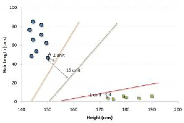
It is a classification method. In this algorithm, we plot each data item as a point in n-dimensional space (where n is number of features you have) with the value of each feature being the value of a particular coordinate. For example, if we only had two features like Height and Hair length of an individual, we’d first plot these two variables in two dimensional space where each point has two co-ordinates (these co-ordinates are known as Support Vectors).
Figure- 1. Without SVM
Figure 2. With SVM
In the example shown above, the line which splits the data into two differently classified groups is the black line, since the two closest points are the farthest apart from the line. This line is our classifier. Then, depending on where the testing data stored on either side of the line, that’s what class we can classify the new data as.
There are 2 key implementations of SVM technique that are mathematical programming and kernel function. It finds an Optimal separates hyper plane between data point of different classes in a high dimensional space. Let’s assume two classes for classification. The classes being P and N for Yn= 1,-1, and by which we can extend to K class classification by using K two class
classifiers. Support vector classifier (SVC) searching hyper plane. But SVC is outlined so kernel functions are introduced in order to non line on decision surface.
Let we is weight vector, his base, Xn is the nearest data point. wT + b >= 1 for xn € P and wTxn + b <= 1 for xn € N. For optimization
the problem minimizes the [WTW] Subject to Yn(WTW +b) >=1 for n=1 to N. The Lagrangian formula for this problem
L[w, b, α] = ||w||2 -anyn(wTxn୬ + b) – 1
A. Strength:
SVM's can model can be used in non-linear decision boundaries, and we can choose various types of kernels. SVM are robust against over fitting and can be implemented in high dimensional space.
B. Weaknesses
Though, SVM are more exhaustive sensitive to switch to the importance of selecting right kernel. It won’t be able to scale over large data sets.
III. INSTANCE LEARNING (lazy learning) APPROACH
The lazy learning i.e. k- means is known as general purpose algorithms that are dependent on clusters with geometric distances that is distance on the coordinate plane between points. The clusters are groups with the centroids marked and causing them to recognize the similar features.
A. K-Nearest Neighbor
KNN can be used for classification problems in the industry. K nearest neighbors is a simple algorithm that stores all available cases and classifies new cases by a majority vote of its k neighbors. The case being assigned to the class is most common amongst its KNN measured by a distance function.
simply assigned to the class of its nearest neighbor. At times, choosing K factor turns out to be a challenge while performing KNN modeling.
KNN can easily be mapped to our real lives. If you want to learn about a person, of whom you have no information, you might like to find out about his close friends and the circles he moves in and gain access to his/her information.
B. Things to Consider Before Selecting KNN
1) KNN is computationally expensive.
2) Variables should be normalized else higher range variables can Bias it.
3) Works on pre-processing stage more before going for KNN like outlier, noise removal.
C. k-Nearest Neighbor Predictions
After selecting the value of ‘k factor’, you can make predictions based on the KNN examples. For regression, a KNN prediction is
the average of the k-nearest neighbor’s outcome.
y ∑ i
Where yi is the ith case of the examples sample and y is the prediction (outcome) of the query point. In classification
problems, KNN predictions are based on a voting scheme in which the winner is used to label the query.
D. Strength:
K factor means is the most decisively clustering algorithm since it's fast, simple, and surprisingly flexible if we pre-process our big data.
E. Weakness
The user has to specify the number of clusters which somehow is not easy to do. If we have any complicated cluster in data is not specified with specific size then K-Means will produce poor clusters.
IV. CONNECTIONIST SYSTEM APPROACH
A. Neural Networks
Neural networks are an underlying framework that act as a supporting structure that follows a model of learning the biological neural networks. Biological neural networks have interconnected neurons with dendrites that receive inputs, then based on these inputs they produce an output signal through an axon to another neuron(SINGH & CHAUHAN, 2009). The process of creating a neural network begins with the most basic form, a single perceptron Neural Network is a set of connected INPUT/OUTPUT UNITS, where each connection has a WEIGHT associated with it. Neural Network learning is also called CONNECTIONIST learning due to the connections between units. Neural Network is always fully connected. It is a case of SUPERVISED, INDUCTIVE or CLASSIFICATION learning. The Weights are adjusted in such a way in Neural Network learning which is able to correctly classify the training data and therefore to classify unknown data in testing phase respectively. It needs long time for training and has a high tolerance to noisy and incomplete data. Learning is being performed by a back propagation algorithm. Concurrently input are passed into input layers. The weighted outputs of these units are,in turn, are fed simultaneously into a “neuron like” units, known as a hidden layer.The weighted output from the hidden layers can be fed input to another hidden layer and so on.The number of hidden layers is arbitrary, but in practice, usually one or two are used. The weighted outputs of the last hidden layer are inputs to units making up the output layer. The most famous training algorithm is the back-propagation algorithm (BP). Back-propagation-type neural networks have an input, an output and, in most of the applications, have one hidden layer. Back-propagation training algorithms of gradient descent and gradient descent with momentum are often too slow for practical problems because they require small learning rates for stable learning. Faster algorithms such as conjugate gradient, quasi-Newton, and Levenberg-Marquardt (LM) use standard numerical optimization techniques. The LM method is in fact an approximation of Newton's method (Shalizi, 2009).
where XR is the original data; Xmin is the minimum of XR; Xmax is the maximum of XR and XN is the result of normalization. The input and target vectors entered the network normalized and the network was trained with these vectors. To train the ANN, no more patterns are necessary. The aim of ANN is to estimate the internal values accurately according to statistical values such as: Linear Correlation Coefficient (R), Mean Squared Error (MSE) (Zare Abyaneh, 2014)the training can be achieved with sufficient data. When the network training was successfully finished, the network was tested using the test data.
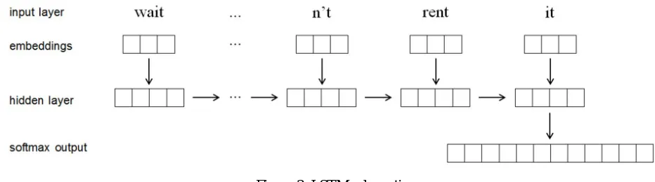
B. LSTM Classifier
The main network architecture we worked on was a recurrent neural network (RNN) with one or more Long-Short Term Memory (LSTM) hidden layer and soft max output layer. The LSTM unit performs the following calculations
it = σ(W(i)xt + U(i)ht-1 + bi)
ft = σ (W(f)xt + U(f)ht-1 + bf )
ot = σ (W(o)xt + U(o)ht-1 + bo) ~ct = tanh(W(c)xt + U(c)ht-1 + bc)
ct = ft ο ct-1 + it ο ~ct ht = otο tanh(ct)
[image:8.612.70.536.350.480.2]and the overall network can be represented as Figure 3.
Figure 3: LSTM schematic
In order to put into the network each word was represented as a skilled 50-dimensional embedding vector. Tweets were input in batch sizes of 32 and either truncated or padded to a length of 120words(the maximum tweets length), with full back-propagation through the entire tweet. Dropout regularization was included during training to prevent over-fitting.
Three versions of the LSTM were compared:
1) Single-Layer, Random Embeddings: The initial model was a single-layer LSTM with randomly initialized word embeddings
2) Single-Layer, Pretrained Twitter Glove Embeddings: Embeddings were instead initialized with GloVe Twitter word embeddings to provide amore informative starting point
3) Double-Layer, Pretrained Twitter Glove Embeddings: A second LSTM hidden layer was added, to potentially capture deeper or more complex dependencies.
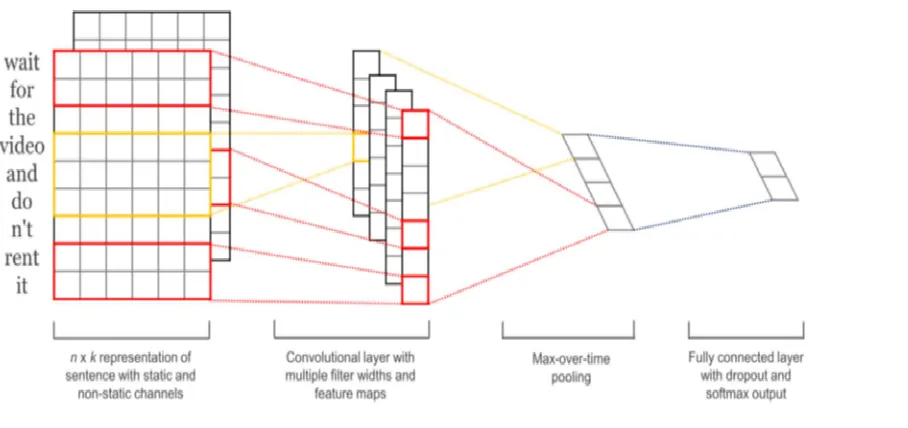
C. CNN Classifier
A convolutional neural network (CNN)(Zeiler & Fergus, 2014). see Figure4. Similarly to the RNN(Sproat & Jaitly, 2016), we utilize word embeddings for each word in the vocabulary, but in this configuration, we reshape each sentence into a 2-D matrix of word embeddings. Let xi 2 Rkbethe k-dimensional word embeddings corresponding to the i-th word in the tweet. The input can be represented as:
where n is the length of the tweet.
We then use 64 filters of size hx50 (where 50 is the size of the embedding) to slide over the embeddings and output features ci. ci = f(w * xi i+h-1 + b)
We use h of size 3, 4, and 5.
The features ci are concatenated, and a max pool is applied per individual filter horizontal slides toobtain ^c = max{c}. Then, these
[image:9.612.90.544.193.407.2]features passed to a fully connected softmax layer whose output is the probability distribution over the emojis. Dropout is also performed for regularization purposes. The static vs. dynamic word channels mentioned in Zeiler et. al. are not implemented here for simplicity.
Figure 4: CNN schematic
D. Strengths
The neural networks had an ability to perform the task in which simple linear program cannot perform. Its having the parallel nature, if an element of a neural network fails, it can be continued without any problem. A neural network does not need to be reprogrammed as it learns itself.
E. Weaknesses
The neural networks require the machine learning training data sets. Requires high processing time for large neural networks.
F. Comparison of LSTMs and CNNs
As it is studied by (Sainath, Vinyals, Senior, & Sak, 2015)architecture uses CNN reduces spectral variation of input feature then passes to the LSTM produces feature representation more easily separable. There is a difference between 4-6% reduction from CNN and LSTM comparatively.
G. Performance Comparisons
We can summarize the performance result of machine learning in following ways:
1) In terms of accuracy Naïve bayes method was the most accurate while artificial immune System and the K- nearest neighbor has the worst precision percentage. In the Rough data set Naïve Bayes has highest performance as compared to K nearest neighbor(E & Wehenkel, 2015).
2) SVM and Naïve Bayes have the highest accuracy which can be regarded as the baseline learning methods(Kharde & Sonawane, 2016).
V. CONCLUSION
In this paper we mainly discuss the classification algorithms which are used for big data analysis. Even these are also related with machine learning concept. We also show how they work on the big data sets, what mathematical concepts they use during analysis purpose. In the future work we will show the comparison of this classification algorithm on large data set, even we will demonstrate which classification performs better during the condition.
REFERENCES
[1] Abellán, J., & Castellano, J. G. (2017). Improving the Naive Bayes classifier via a quick variable selection method using maximum of entropy. Entropy, 19(6). https://doi.org/10.3390/e19060247
[2] Abellán, J., Klir, G. J., & Moral, S. (2006). Disaggregated total uncertainty measure for credal sets. International Journal of General Systems, 35(1), 29–44. https://doi.org/10.1080/03081070500473490
[3] E, D. E. S. S. C. a P., & Wehenkel, L. (2015). M ACHINE L EARNING A PPROACHES TO par, 2(1), 1–12.Gupta, R. (2015). MACHINE LEARNING Raghav Agarwal, (11), 1342–1347.
[4] Gupte, A., Joshi, S., Gadgul, P., & Kadam, A. (2014). Comparative Study of Classification Algorithms used in Sentiment Analysis. (IJCSIT) International Journal of Computer Science and Information Technologies, 5(5), 6261–6264
[5] Juan, a, Vilar, D., & Ney, H. (2007). Bridging the Gap between Naive Bayes andMaximum Entropy Text Classificatio. Pris, 1, 59--65. Retrieved from http://dl.acm.org/citation.cfm?id=234289%5Cnhttp://www-i6.informatik.rwth-aachen.de/publications/download/272/Juan-PRIS-2007.pd
[6] Kashyap, H., & Buksh, B. (2016). Combining Naïve Bayes and Modified Maximum Entropy Classifiers for Text Classification. International Journal of Information Technology and Computer Science, 8(9), 32–38. https://doi.org/10.5815/ijitcs.2016.09.0
[7] Kharde, V. A., & Sonawane, S. S. (2016). Sentiment Analysis of Twitter Data: A Survey of Techniques. International Journal of Computer Applications, 139(11), 975–8887. https://doi.org/10.5120/ijca2016908625Mitchell, T. M. (2011). Machine Learning 10-701. Machine Learning, 1–14
[8] Pradhan, A. (2012). SUPPORT VECTOR MACHINE-A Survey. International Journal of Emerging Technology and Advanced Engineering, 2(8), 82–85. Retrieved from http://www.ijetae.com/files/Volume2Issue8/IJETAE_0812_11.pd
[9] Sainath, T., Vinyals, O., Senior, A., & Sak, H. (2015). Convolutional, Long Short-Term Memory, fully connected Deep Neural Networks. ICASSP, IEEE International Conference on Acoustics, Speech and Signal Processing - Proceedings, 2015–Augus, 4580–4584. https://doi.org/10.1109/ICASSP.2015.717883 [10] Shalizi, C. (2009). Logistic Regression and Newton ’ s Method, 7(November), 1–12. Retrieved from
http://www.stat.cmu.edu/~cshalizi/350/lectures/26/lecture-26.pd
[11] Shannon, C. E. (1948). A mathematical theory of communication. The Bell System Technical Journal, 27(July 1928), 379–423. https://doi.org/10.1145/584091.58409
[12] SINGH, D. Y., & CHAUHAN, A. S. (2009). Neural Networks In Data Mining. Journal of Theoretical and Applied Information Technology, 5(1), 1–154 [13] Sproat, R., & Jaitly, N. (2016). RNN Approaches to Text Normalization: A Challenge. ArXiv
[14] Tan, P.-N., Steinbach, M., & Kumar, V. (2005). Cluster Analysis: Basic Concepts and Algorithms. In Introduction to Data Mining (p. Chapter 8). https://doi.org/10.1016/0022-4405(81)90007-
[15] Tsai, C.-W., Lai, C.-F., Chao, H.-C., & Vasilakos, A. V. (2015). Big data analytics: a survey. Journal of Big Data, 2(1), 2https://doi.org/10.1186/s40537-015-0030-
[16] Vadivukarassi, M., Puviarasan, N., & Aruna, P. (2017). Sentimental Analysis of Tweets Using Naive Bayes Algorithm, 35(1), 54–59. https://doi.org/10.5829/idosi.wasj.2017.54.5
[17] Walters-Williams, J., & Li, Y. (2010). Comparative study of distance functions for nearest neighbors. In Advanced Techniques in Computing Sciences and Software Engineering (pp. 79–84). https://doi.org/10.1007/978-90-481-3660-5-1
[18] Zare Abyaneh, H. (2014). Evaluation of multivariate linear regression and artificial neural networks in prediction of water quality parameters. Journal of Environmental Health Science & Engineering, 12(1), 40. https://doi.org/10.1186/2052-336X-12-4