Mixing times for exclusion processes on hypergraphs

White Rose Research Online URL for this paper:

http://eprints.whiterose.ac.uk/147108/

Version: Published Version

Article:

Connor, Stephen Bryan orcid.org/0000-0002-9785-2159 and Pymar, Richard (2019) Mixing

times for exclusion processes on hypergraphs. Electronic Journal of Probability. 73. ISSN

1083-6489

https://doi.org/10.1214/19-EJP332

[email protected]

https://eprints.whiterose.ac.uk/

Reuse

This article is distributed under the terms of the Creative Commons Attribution (CC BY) licence. This licence

allows you to distribute, remix, tweak, and build upon the work, even commercially, as long as you credit the

authors for the original work. More information and the full terms of the licence here:

https://creativecommons.org/licenses/

Takedown

If you consider content in White Rose Research Online to be in breach of UK law, please notify us by

El e c t ro n ic

J

o f

P r

o

b a b_{i l i t y}

Electron. J. Probab.24(2019), no. 73, 1–48. ISSN:1083-6489 https://doi.org/10.1214/19-EJP332

Mixing times for exclusion processes on hypergraphs

Stephen B. Connor

Richard J. Pymar

Abstract

We introduce a natural extension of the exclusion process to hypergraphs and prove an upper bound for its mixing time. In particular we show the existence of a constant

Csuch that for any connected, regular hypergraphGwithin some natural class, the

ε-mixing time of the exclusion process onGwith any feasible number of particles can be upper-bounded byCTEX(2,G)log(|V|/ε), where|V|is the number of vertices

inGandTEX(2,G)is the 1/4-mixing time of the corresponding exclusion process with

just two particles. Moreover we show this is optimal in the sense that there exist hypergraphs in the same class for whichTEX(2,G) and the mixing time of just one

particle are not comparable. The proofs involve an adaptation of the chameleon process, a technical tool invented by Morris ([14]) and developed by Oliveira ([15]) for studying the exclusion process on a graph.

Keywords:mixing time; exclusion; interchange; random walk; hypergraph; coupling.

AMS MSC 2010:Primary 60J27; 60K35, Secondary 82C22.

Submitted to EJP on March 23, 2018, final version accepted on June 9, 2019. SupersedesarXiv:1606.02703v4.

1

Introduction

Let G = (V, E) be a finite connected graph with vertex set V and edge set E. Fixk ∈ {1, . . . ,|V|}and considerk indistinguishable particles moving onV using the following rules:

1. each vertex is occupied by at most one particle,

2. each edgee∈Erings at the times of a Poisson process of rate 1, independently of all other edges,

*_{Both authors supported in part by LMS Research in Pairs (Scheme 4) Grant 41215. SBC supported in part}

by EPSRC Research Grant EP/J009180. RJP supported in part by Leverhulme Research Grant RPG-2012-608 held by Nadia Sidorova and EPSRC Grant EP/M027694/1 held by Codina Cotar.

†_{Department of Mathematics, University of York, York, YO10 5DD, UK. E-mail:[email protected]} ‡_{Department of Economics, Mathematics and Statistics, Birkbeck, University of London, London, WC1E}

3. when an edge e = {u, v} rings, the occupancy states of vertices u and v are switched.

For eachv∈V andt≥0, letηt(v) = 1ifvis occupied at timet, andηt(v) = 0ifvis

vacant at timet. The process(ηt)t≥0is called thek-particle exclusion process onG: see

Figure 1. In this paper we are interested in a natural extension of the exclusion process tohypergraphs.

Figure 1: Example transition of 3-particle exclusion process onK5. When the edge

indicated rings, the single particle currently on that edge moves to the vertex at the other end of the edge.

LetG= (V, E)be a finite connected hypergraph, whereE ⊆ P(V), the power set ofV. For eache∈E, denote bySethe symmetric group on the elements ine, and let

fe:Se→[0,1]be a probability measure onSe. We writef to denote{fe: e∈E}, the

set of these measures. Considerkindistinguishable particles moving onV using rules 1. and 2. above and in addition:

3′. when an edgeerings, a permutationσ∈ Seis chosen according tofeand every

particle on a vertex in e moves simultaneously according to σ, i.e. a particle at vertex v moves to vertex σ(v). (Note that as σ is a permutation, rule 1. is preserved.)

Settingηt(v) = 1ifvis occupied at timetand 0 otherwise, we obtain a process(ηt)t≥0

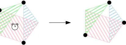
referred to as thek-particle exclusion process on(f, G), or simply EX(k, f, G): see Figure 2. (Note that if each edgee ∈ E contains exactly two vertices, and fe puts all of its

mass on the transposition belonging toSe, then EX(k, f, G) is just thek-particle exclusion

process on the graphG, as above.)

Figure 2: Example transition of 3-particle exclusion process on a hypergraph with 5 vertices and 3 edges (indicated by the different shaded regions, i.e. here there are two edges of size 3 and one of size 4). When the edge containing four vertices rings, the two particles currently belonging to that edge are permuted.

Our main aim in this paper is to study the total-variation mixing time of EX(k, f, G), and to establish an upper bound in terms of the mixing time of EX(2, f, G). Recall that for a continuous-time Markov processX on a finite setΩwith transition probabilities {qt(x, y)}and equilibrium distributionπ, the total variationε-mixing time is defined as

TX(ε) := inf

t≥0 : max

x∈Ωkqt(x,·)−πkTV≤ε

wherek · kTVis the total-variation norm.

In several parts of the proof it will be useful to consider the associated process where thekparticles are distinguishable. Suppose the particles are labelled1, . . . , kand set ˆ

ηt(v) to be the label of the particle at vertexv at time t. If there is no particle atv

at timet, setηˆt(v) = 0. The process(ˆηt)t≥0 is the k-particle interchange process on

(f, G), or simply IP(k, f, G). Note that the exclusion process may be recovered from the interchange process simply by ‘forgetting’ the labels of the particles.

Throughout we will make the following assumptions about the hypergraphGand the set of measuresf (with notation appearing below being formally defined in Section 2.1).

Assumption 1.1.

1. The hypergraphGis regular (every vertex has the same degree).

2. For everye,feis constant on the conjugacy classes ofSe(i.e. in group-theoretic

terms,feis a class function). That is, ifσ1andσ2 are elements fromSewith the

same cycle structure, thenfe(σ1) =fe(σ2).

3. For every e and each v ∈ e, P_σ∈S

efe(σ)1{σ(v)=v} ≤ 1/5. In other words, the probability (underfe) of a vertexv∈ebeing a fixed point ofσis at most1/5.

4. The interchange process IP(k, f, G) is irreducible for any number of particles

k∈ {1, . . . ,|V| −1}.

These assumptions are more than enough to imply that the exclusion process is reversible and ergodic, with uniform stationary distribution. Although we state it as an assumption onf, the fourth assumption also implies that the underlying hypergraphG

is connected. Our main theorem is the following:

Theorem 1.2.There exists a universal constantC >0such that for every(f, G) satisfy-ing Assumption 1.1 and everyk∈ {1, . . . ,|V| −1}andε >0,

TEX(k,f,G)(ε)≤Clog(|V|/ε)TEX(2,f,G)(1/4).

Remark 1.3.In all further statements we implicitly assume that Assumption 1.1 holds.

Remark 1.4.The exclusion process on a hypergraphGwith the edge setEconsisting only of edges of size 2 or 3 exhibits thenegative correlationproperty (which we shall discuss further in the sequel). As a result, for this subset of hypergraphs we can actually extend the main theorem, replacing theTEX(2,f,G)(1/4)appearing in the

right-hand side byTEX(1,f,G)(1/4) (note that we later refer toEX(1, f, G)as RW(1, f, G), in

recognition that the exclusion process with just one particle is equivalent to a single particle performing a random walk).

Remark 1.5.A simple example suffices to show that Theorem 1.2 is optimal in the sense that we cannot replaceTEX(2,f,G)(1/4)on the right-hand side withTEX(1,f,G)(1/4)(even

under our standing assumptions). LetG= (V, E)withV ={1,1′,2,2′, . . . , m, m′}and

E={{i, i′_{, j, j}′_{}: i6=j}. Suppose thatf}

{1,1′_,2,2′_}(σ) = 1/6ifσis a cycle of size 4 (and

otherwisef{1,1′_,2,2′_}(σ) = 0). For{i, i′, j, j′} 6={1,1′,2,2′}, we setf_{i,i′_,j,j′_}(σ) = 1/3ifσ

is a composition of two disjoint transpositions (and otherwisef{i,i′_,j,j′_}(σ) = 0). It can

be readily checked that this hypergraph satisfies Assumption 1.1. Note that there are

m

2

edges, each ringing at rate 1. It is easy to see that a random walker mixes in time of order1/msince each vertex is in ordermedges. Now consider a 2-particle exclusion process started from{3,3′_{}. Notice that up until the first time that both particles occupy}

vertices belonging to the edge{1,1′_,2,2′_{}, if vertexiis occupied then vertexi}′_{is also}

occupied. So the process cannot mix until the edge{1,1′_,2,2′_{}is visited by the particles.}

can ring which would bring the particles to the set{1,1′,2,2′}, and so this happens at rate 2; we conclude that it takes a time of order 1 for the 2-particle exclusion process to mix.

1.1 Motivation and connections with the literature

Our results contribute to the general question of when properties of a multi-particle system can be deduced from properties of a system with only a few particles. Arguably the most significant recent result in this area has come from Caputo, Liggett and Richthammer ([3]) who showed that the spectral gap of the interchange process on a graph is equal to the spectral gap of a random walker on the same graph, proving a conjecture of Aldous that had been open for 20 years. Proving results in this area is particularly important in applications since the large reduction in the size of the state space often makes it much easier to compute or estimate statistics.

While interacting particle system models (e.g. exclusion process, interchange process, voter model, contact process, zero range process) on graphs have received considerable attention, there has so far been little study of such processes on hypergraphs. Studying these processes on hypergraphs is very natural though, as hypergraphs allow simultane-ous interactions of multiple particles, rather than only pair-wise interactions. One model for which its analogue on hypergraphs has been recently studied is the voter model ([4, 8]), for which various properties are considered, including the mixing time.

Any interchange process (withk=|V|) on a graph can be viewed as a card shuffle by transpositions, and there is now an extensive literature concerning mixing times of such shuffles. Notable examples include the top-to-random transposition shuffle (star graph; [6]), random-to-random transposition shuffle (complete graph; [5]) and nearest-neighbour transposition shuffle (the cycle; [9]). Of course, transposition shuffles are just one class of shuffle, and there is significant interest in mixing times of more general shuffles in which multiple cards are moved simultaneously. A large class of time-homogeneous shuffles can be represented as interchange processes on hypergraphs; recent examples can be found in [2] and [7].

Achieving tight bounds on the mixing time of an interacting particle system typically involves finding an argument tailored specifically to the model in question. If we care less about the specific constant multiple (at which mixing occurs) and instead focus on the order, a result of Oliveira ([15]) can prove particularly useful as a general way of bounding mixing times of exclusion processes:

Theorem 1.6 ([15]).There exists a constant C > 0 such that for every connected weighted graphGand everyk∈ {1, . . . ,|V| −1}andε∈(0,1/2),

TEX(k,G)(ε)≤Clog(|V|/ε)TRW(G)(1/4),

whereTRW(G)(1/4)is the mixing time of the random walk onG.

Our main result extends Theorem 1.6 to a class of hypergraphs. Furthermore, our results hold for a large class of measures acting on the symmetric groupS|V|which goes

beyond the standard framework studied by previous authors, in which a conjugacy class is fixed and then sampled from uniformly (e.g. [13, 2]). Indeed, our measuresfecan

vary dramatically between edgese∈E, and furthermore we do not require eachfeto

be supported on a fixed conjugacy class.

1.2 Heuristics and structure of the proof

The proof of Theorem 1.2 depends on the size of the vertex setV. If|V|is sufficiently small, the proof is fairly simple and we state the result as the following lemma:

with|V|<36, everyf and everyk∈ {1, . . . ,|V|/2}andε >0,

TEX(k,f,G)(ε)≤Clog(1/ε)TEX(2,f,G)(1/4).

On the other hand, the argument for|V| ≥36is much more intricate and is split into two parts, the first being the following lemma which is of independent interest (and is stronger than needed for our main theorem, as it relates to the interchange process):

Lemma 1.8.There exists a constantC >0such that for every hypergraphG= (V, E) with|V| ≥36, everyf and everyk∈ {1, . . . ,|V|/2}andε >0,

TIP(k,f,G)(ε)≤Clog(|V|/ε)TEX(4,f,G)(1/4).

Oliveira ([15]) proves his main result (bounding the mixing time of the k-particle exclusion process by the mixing time of a random walker) by first relating the mixing time of a k-particle interchange process to that of a 2-particle interchange process. Roughly speaking, this is possible due to the fact that any time an edge of the graph under consideration rings, at most two particles move under interchange, and so it is pairwise interactions that determine the mixing rate. This contrasts with the exclusion process on hypergraphs considered here, in whichmany particles can move at the same time. Nevertheless, a suitable adaptation of the techniques appearing in [15] provides the proof of Lemma 1.8.

Remark 1.9.Lemma 1.8 only holds when|V|is sufficiently large and k≤ |V|/2. We cannot hope to remove these conditions and replace EX(4, f, G)with EX(2, f, G)in this statement, even for hypergraphs satisfying Assumption 1.1, as the following example illustrates. LetG= (V, E)withV ={1,2,3}andE={V}, i.e. there is just a single edge which contains all three vertices in the hypergraph. Suppose thatfgives probability1−δ

to the conjugacy class of 3-cycles, and probabilityδto the class of transpositions. Forδ

sufficiently small this satisfies Assumption 1.1. The 2-particle interchange process cannot mix until a transposition is chosen (as half of the states cannot be reached before this time), whereas this event is not necessary for the 2-particle exclusion process to mix, and hence it is straightforward to see that asδ→0we haveTIP(2,f,G)(1/4)/TEX(2,f,G)(1/4)→

∞.

The second part of the proof for |V| ≥ 36 requires showing that TEX(4,f,G) and

TEX(2,f,G)are of the same order:

Lemma 1.10.There exists a constant λ > 0 such that for any hypergraph G with |V| ≥36, andf,

TEX(4,f,G)(1/4)≤λTEX(2,f,G)(1/4).

We now demonstrate that Theorem 1.2 follows simply from Lemmas 1.7, 1.8 and 1.10.

Proof of Theorem 1.2. The contraction principle (see [1]) gives

TEX(k,f,G)(ε)≤TIP(k,f,G)(ε),

and so providedk ≤ |V|/2, we have the result for|V| ≥ 36by Lemmas 1.8 and 1.10 and for|V|<36by Lemma 1.7. However, note that switching the roles of occupied and unoccupied vertices in EX(k, f, G)yields the process EX(|V| −k, f, G). It follows that

TEX(k,f,G)(ε) =TEX(|V|−k,f,G)(ε),

We finish this section with a brief overview of the rest of the paper. In Section 2 we define formally the processes considered in this paper and present some preliminary results. In addition, we demonstrate that the negative correlation property, which is fundamental to the result in [15], fails to hold for the hypergraph setting. In Section 3 we prove Lemma 1.8 subject to the existence of a process with certain key properties that relate it to an interchange process: see Lemma 3.1 for the precise statement. This process is constructed in Section 6 and we show it has the desired properties in Section 7. Proving Lemma 3.1 is the most challenging (and technical) part of this paper.

In Section 4 we prove Lemma 1.10 by first characterizing every hypergraph as one of two types depending on how long it takes any two of four independent particles to meet.

We use some of the ideas developed in Section 4 to prove Lemma 1.7 in Section 5. A few of the more technical proofs required are included in two appendices.

2

Preliminaries

2.1 Random walks, exclusion and interchange processes

We formally define the main processes studied in this paper, RW(f, G), RW(k, f, G), EX(k, f, G) and IP(k, f, G), by explicitly stating their generators. In the next section we shall present agraphical construction of these processes, similar to that of Liggett ([12]) for the standard interchange and exclusion processes. This graphical construction will allow us to simultaneously define the processes on the same probability space, and thus directly compare them.

RecallSeas the group of permutations of elements ine. Our processes of interest

evolve by the action of permutations from these groups. However, it will often be convenient to consider permutations as acting on V and we can easily do this by extending a permutation σe ∈ Se to a permutation inSV by settingσe(v) =v for all

v /∈e. We can also consider such permutations as acting on a subset ofV or on vectors with elements being distinct members ofV. To do this we can define, for a setA⊆V,

σe(A) := {σe(a) : a ∈ A}, and for a vector x of k distinct elements ofV we define

σe(x) := (σe(x(i)))ki=1.

Set notation:Fork∈Nwe define

V k

:={A⊆V : |A|=k},

and for a setA⊆V we write

(A)k:={a= (a(1), . . . ,a(k))∈Ak : a(i)6=a(j)∀i6=j}.

Generators: We now explicitly state the generators of the processes. For a hyper-graphGand a suitable set of functionsf, the simple random walk onG, RW(f, G), is the continuous-time Markov chain with state spaceV and generator

URW_{h(u) =}X

e∈E

X

σ∈Se

fe(σ)(h(σ(u))−h(u))

for allu∈V andh:V →R.

We denote by RW(k, f, G)the product ofkindependent random walkers onG. This process is the continuous-time Markov chain with state spaceVk_{and generator}

URW(k)_{h(u) =}X

e∈E k

X

i=1

X

σ∈Se

for allu∈Vk andh:Vk→R, where

ui_v(j) = (

u(j) j6=i,

v j=i.

Thek-particle exclusion process EX(k, f, G), is the continuous-time Markov chain with state space V_kand generator

UEX_{h(A) =}X

e∈E

X

σ∈Se

fe(σ)(h(σ(A))−h(A)),

for allA∈ V_kandh: V_k→R.

Thek-particle interchange process IP(k, f, G), is the continuous-time Markov chain with state space(V)k and generator

UIP_{h(x) =}X

e∈E

X

σ∈Se

fe(σ)(h(σ(x))−h(x)),

for allx∈(V)k andh: (V)k →R.

2.2 Graphical construction

We first construct an independent sequence ofE-valued random variables{en}n∈N

such that eachenis identically distributed withP[en=e] = 1/|E|. Given the sequence

{en}n∈N, let{σ_n}_n∈Nbe a sequence of permutations withσ_n∈ S_enindependently chosen

and satisfying for eachn∈N, ande∈E,P_{[σn =σ|en=e] =fe(σ)}. Now that we have the sequence of edges that ring and the permutations to apply, it remains to determine the update times of the processes.

Let Λ be a Poisson process of rate |E| and for 0 < s < t denote by Λ[s, t] the number of points ofΛin [s, t]. For every0 < s < t, we define a random permutation

I[s,t] : V → V associated with the time interval [s, t] to be the composition of the

permutations performed during this time; that is,

I[s,t]=σeΛ[0,t]◦σeΛ[0,t]−1◦ · · · ◦σeΛ[0,s)+1.

We setIt:=I[0,t]for eacht >0, andI(t,t] to be the identity. Note (cf Proposition 3.2 of

[15]) that

L[I(s,t]] =L[I(−s,t1]], (2.1)

where we writeLfor the law of a process.

We can lift the functionsI[s,t]to functions on V_k

and(V)k in the following way: for

A∈ V_k,

I[s,t](A) ={I[s,t](a) : a∈A},

and forx∈(V)k,

I[s,t](x) = (I[s,t](x(1)), . . . , I[s,t](x(k))).

The following proposition is fundamental: its proof follows by inspection.

Proposition 2.1.Fixs >0. Then:

1. For eachu∈V, the process{I[s,s+t](u)}t≥0is a realisation ofRW(f, G)initialised

atuat times. We shall often write this process simply as(uRW

t )t≥s.

2. For each A ∈ V_k, the process{I[s,s+t](A)}t≥0 is a realisation of EX(k, f, G)

ini-tialised atAat times. We shall often write this process simply as(AEXt )t≥s.

3. For each x ∈ (V)k, the process {I[s,s+t](x)}t≥0 is a realisation of IP(k, f, G)

2.3 Total variation and mixing times

There are several equivalent definitions of total variation that we shall make use of in this paper. Supposeµandν are two probability measures on the same finite setΩ. Then thetotal variation distance between these measures is defined as

kµ−νkTV := max

A⊂Ω(µ(A)−ν(A)) (2.2)

= sup

f:Ω→[0,1]

Z

f dµ− Z

f dν. (2.3)

We shall also make extensive use of the following equivalent definition, which relates the total variation distance to couplings ofµandν:

kµ−νkTV = inf (X,Y)

P_{[X 6=Y],} (2.4)

where the infimum is over all couplings (X, Y)of random variables with X ∼ µand

Y ∼ν. We recall a simple result bounding the total variation of product chains (see e.g. pg 59 of [10]): forn∈Nand1≤i≤n, letµi andνi be measures on a finite spaceΩi

and define measuresµandνonQn_i=1Ωibyµ:=Qn_i=1µiandν :=Qn_i−1νi. Then

kµ−νkTV≤

n

X

i=1

kµi−νikTV. (2.5)

Recall equation (1.1) as the definition of the mixing time of a continuous-time Markov process. We will require several general mixing-time bounds throughout this work, which we present here.

Proposition 2.2 ([10]).LetX be a Markov process on a finite state space. Then for everyε1, ε2∈(0,1/2),

TX(ε2)≤

logε2

log(2ε1)

TX(ε1).

Proposition 2.3.For anym, n∈N,

TRW(2m_,f,G)(2−n)≤(n+m)T_RW(f,G)(1/4).

Proof. This follows by combining Proposition 2.2 with (2.5).

Proposition 2.4([1]).LetX be a Markov process on a finite state spaceΩwith sym-metric transition rates. Then the equilibrium distribution is uniform overΩand for all 0< ε <1/2andt≥2TX(ε),

P_{[Xt=ω2|X0=ω1]≥} (1−2ε)

2

|Ω| ,

for allω1, ω2∈Ω.

2.4 Failure of negative correlation

We conclude this preliminary section with a quick example to demonstrate that the exclusion process on a hypergraph does not enjoy the negative correlation property satisfied by the exclusion process on a graph. We first recall the version of the negative correlation property of the exclusion process on a graph to which we refer, and whose proof may be found in [11]. Let B ⊂ V and let (AEX

t )t≥0 be a 2-particle exclusion

process on a graphG= (V, E)withA={u, v}. Suppose(uRW

independent realisations of RW(1, f, G), started fromuandvrespectively. Then for every

t≥0,

P_AEX_{t ⊆B≤}P_utRW_∈BP_vtRW_∈B.

Now suppose G= (V, E)is the hypergraph with V ={1,2,3,4} andE ={V} (i.e. there is only one edge), and thatf is concentrated uniformly on the six possible 4-cycles. Let(AEX

t )t≥0be a realisation of EX(2, f, G), withA={u, v}={1,2}, and letB={3,4}.

We claim that there exist values oftsuch that

P_uRW_{t ∈B, vt}RW _∈B<P_AEX_{t =B.} (2.6)

Indeed, since the event{uRW

t ∈B}is less likely than seeing at least one incident in a

unit-rate Poisson process by timet, we have

P_uRW_{t ∈B, vt}RW_∈B=P_uRW_{t ∈B}P_vtRW_{∈B≤(1−e}−t₎2_.

On the other hand, the event{AEX

t =B}is at least as likely as the edge ringing exactly

once by timet, with the chosen permutation satisfyingσ({1,2}) ={3,4}. That is,

P_AEX_{t =B≥} 1 3te

−t_.

Inequality (2.6) is therefore satisfied for anyt <0.33.

3

From

k

_{-particle interchange to 4-particle exclusion}

In this section we shall prove Lemma 1.8. Given a hypergraph with vertex setV and a(k−1)-tuplez∈(V)k−1, let

O(z) :={z(1), . . . ,z(k−1)}

be the (unordered) set of coordinates ofzand define a space

Ωk(V) :={(z, R, P, W) : z∈(V)k−1, and setsO(z), R, P, W partitionV}.

As we shall see, most of the work required to prove Lemma 1.8 is to show the existence of a certain Markov process having some key properties, which we outline in the Lemma 3.1 below. As we shall see in the sequel, this Markov process is very similar to the chameleon process used in [15] and it provides a way of tracking how mixed thekth particle is in ak-particle interchange process. Thekth particle is replaced by three sets of coloured particles,Rt(red particles),Pt(pink particles) andWt(white

particles), with the colours informing the conditional distribution of thekth particle in the interchange process. A process(inkx

t(b))t≥0is defined for each vertexb∈V, which

records the amount ofrednessat vertexb(equal to 1 if a red particle is at vertexband 1/2 if a pink particle is at vertex b). We shall also define an eventFillx _{as the event}

that all vertices unoccupied by the firstk−1particles in the interchange process are eventually each occupied by a red particle in the chameleon process.

Lemma 3.1.There exist constantsc1, c2andκ1such that for every regular hypergraph

G= (V, E)with|V| ≥36, everyf, everyk∈ {2, . . . ,|V|/2}, everyx= (z, x)∈(V)k, and

every realisation(xIP

t )t≥0of IP(k, f, G)started from statex, there exists a

continuous-time Markov process(Mt)t≥0 := (zCt, Rt, Pt, Wt)t≥0 with state-spaceΩk(V)defined on

the same probability space as(xIP_t )t≥0satisfying:

2. for everyt≥0andb= (c, b)∈(V)k,

PxIP_t =b=E

h inkx

t(b)1_{zC_t=c}

i

,

whereinkx

t(b) :=1{b∈Rt}+

1

21{b∈Pt}; 3. for everyt≥0andj ∈N_,

E

1− ink x

t

|V| −k+ 1 Fillx

≤c1

p

|V|e−c2j_{+ exp}

j− t

κ1TEX(4,f,G)(1/4)

whereinkx

t :=

P

b∈V ink

x

t(b)andFillx:={limt→∞inkxt =|V| −k+ 1};

4. for everyt≥0andc∈(V)k−1,

P_{zC_t =c} ∩Fillx = P

zC_t =c

|V| −k+ 1.

The proof of Lemma 3.1 is deferred to Section 7 and is a proof by construction: in Section 6 we will explicitly define a process and then proceed to show that it has the desired properties. We can now relate the total-variation distance between two realisations ofIP(k, f, G)to a certain expectation involving the amount of ink in the chameleon processM in the statement of Lemma 3.1. The following result is similar to Lemma 6.1 of [15]: we include a sketch of the proof to highlight the importance of constructing in Section 6 a chameleon process satisfying part 2 of Lemma 3.1.

Lemma 3.2.For everyt≥0,

sup x,y∈(V)k

kL[xIP_t ]− L[yIP_t ]kTV≤2k sup

w∈(V)k E

1− ink w

t

|V| −k+ 1 Fillw

Proof. Fixx= (z, x)∈(V)k withz∈(V)k−1, and denote byxIPt an interchange process

started fromx. Letx˜be uniform fromV\O(z)and denote byx˜IP_t an interchange process started fromx˜ = (z,x˜). Then for anyb= (c, b)∈(V)k,

Px˜IP_t =b=P

zIP

t =c

|V| −k+ 1 = PzC

t =c

|V| −k+ 1 =P

{zC_t =c} ∩Fillx ,

where the second and third equalities follow from parts 1 and 4 of Lemma 3.1, respec-tively. On the other hand, part 2 of Lemma 3.1 gives

PxIP_t =b=E_[inkx

t(b)1_{zCt=c}]≥E[ink x

t(b)1_{{ztC=c}∩Fillx}].

Subtracting we obtain

Px_˜IP_t =b−PxIP_t =b≤E_[(1−inkx

t(b))1_{{ztC=c}∩Fillx}].

Hence

kL[xIP_t ]− L[˜xIP_t ]kTV≤

X

(c,b)∈(V)k

E_[(1−inkx

t(b))1_{{zCt=c}∩Fillx}]

=E_{[(|V| −k+ 1−ink}x

t)1{Fillx_}]

=E

1− ink x

t

|V| −k+ 1 Fillx

.

Proof of Lemma 1.8. We combine part 3 of Lemma 3.1 with Lemma 3.2 to give for every

t≥0andj ∈N,

sup x,y∈(V)k

kL[xIP_t ]− L[yIP_t ]kTV≤2k

c1

p

|V|e−c2j_{+ exp}

j− t

κ1TEX(4,f,G)(1/4)

,

for some universal positive constantsc1, c2andκ1. We choose

j=

t

(1 +c2)κ1TEX(4,f,G)(1/4)

,

which gives the bound (usingk≤ |V|),

sup x,y∈(V)k

kL[xIP_t ]− L[y_tIP]kTV ≤c3|V|3/2exp

−c2t

(1 +c2)κ1TEX(4,f,G)(1/4)

,

for some positivec3. Therefore there exists a universal constantCsuch that for any

ε∈(0,1/2)andt > CTEX(4,f,G)(1/4) log(|V|/ε),

sup x,y∈(V)k

kL[xIP_t ]− L[y_tIP]kTV ≤ε.

4

From 4-particle exclusion to 2-particle exclusion

In this section we shall prove Lemma 1.10. We begin by characterizing every con-nected hypergraph in terms of how long it takes two independent random walkers on the hypergraph to arrive onto the same edge, which then rings for one of the walkers – a time we shall refer to as themeeting time of the two walkers (note that we do not require the two walkers to actually occupy the same vertex). It will be useful to consider such times, as we will be able to couple two independent walkers with a 2-particle interchange process, up until this meeting time (see Proposition 4.7 for this statement).

Formalising this, fory∈V2_{, let(y}RW

t )t≥0be a realisation of RW(2, f, G)withyRW0 =y.

Denote byΛ1_andΛ2_{the Poisson processes used to generate the edge-ringing times for}

the two particles, and let{e1

n}n∈N and{e2_n}_n∈N be the two sequences of edge-choices

(all as in Section 2.2). DefineMRW_{(y)to be the first timey}RW

t (1)andytRW(2)are in the

same edge which then rings in one of the processes:

MRW(y) := inft >0 : ∃e∈ {e1Λ1_[0,t], e2_Λ2_[0,t]}withyRW_t− (1),y_tRW₋ (2)∈e . (4.1)

Definition 4.1.We say that a hypergraphGiseasyif

sup y∈V2

P_MRW₍y)>1010TEX(2,f,G)(1/4)

≤1/1000.

Remark 4.2.We note that this definition is similar to Definition 4.1 in [15], from where we borrow the dichotomy “easy/non-easy”. However, for the case of hypergraphs, this characterisation does not reflect the associated difficulty of dealing with each case! One difference in the case of hypergraphs is that at the meeting time we cannot guarantee that the two independent walkers occupy the same site, and this results in the analysis being more challenging.

4.1 From 4-particle exclusion to 2-particle exclusion: easy hypergraphs

thekth particles meet on an edge of size at least 5 and the permutation chosen at this meeting time does not fix thekth particles.

LetΛbe a Poisson process of rate2|E|(i.e. twice the usual rate), with associated edge-choices {en}n∈N and permutations {σ_n}_n∈N as in Section 2.2. In addition, let {θn}n∈N be an i.i.d. sequence of Bernoulli(1/2)random variables: these will be used to

thin the events ofΛand ensure that all particles are moving at the correct rate. We write ˆ

Λfor the thinned Poisson process obtained fromΛby removing all points corresponding toθn = 0. LetIˆtbe constructed fromΛˆ as in Section 2.2. We make this modification as it

allows us to more easily compare a certain time to the meeting time of two independent random walkers as defined in (4.1).

Lemma 4.3.LetD ∈ _kV₋₁, a, b∈V \DandA=D∪ {a},B =D∪ {b}. Let(AEXc

t )t≥0

and(BEXc

t )t≥0be two realisations of EX(k, f, G)started fromAandB respectively and

evolving according toIˆt. Let

τa,b:= inf{t≥0 : ˆIt(a),Iˆt(b)∈eΛ[0,t]},

and writeea,b foreΛ[0,τa,b] andσa,b forσΛ[0,τa,b]. Write alsoa

∗ _forIˆ

[0,τa,b)(a)andb

∗ _for

ˆ

I[0,τa,b)(b). Then there exist two other realisations of EX(k, f, G)denoted(A

f

EX

t )t≥0and

(BEX

t )t≥0which start and evolve identically to(AEXtc)t≥0and(BtEXc)t≥0respectively up to

timeτa,b−but which satisfy, on the event

{σa,b(a∗)6=a∗} ∩ {|ea,b|>4},

with probability at least ₂₅2,AEXtf =BtEXfor allt≥τa,b.

Proof. We define two events which will be used to determine the coupling strategy of the processes(AEXf

t )t≥0and(BtEX)t≥0at timeτa,b:

J1(σa,b) =

σa,b(a∗)∈ {/ a∗, b∗}, σa,b(b∗)∈ {/ a∗, b∗}

J2(σa,b) =J1(σa,b)∩

n_ˆ

Iτa,b−(D)∩σa,b(a

∗_)=Iˆ

τa,b−(D)∩σa,b(b

∗₎o_.

In words,J1(σa,b)is the event that the permutationσa,b moves the set of two ‘special’

particles (those initially at vertices aand b) to a new set of positions; event J2(σa,b)

further specifies that the two positions to whichσa,bmoves the special particles should

either both contain another particle (i.e. one of the already-matchedk−1particles) or both be empty.

With this notation in place, we can describe the coupling at timeτa,b:

(i) ifθa,b= 0then we do not update the processes at timeτa,b;

(ii) ifθa,b = 1but eventJ2(σa,b)fails to hold, then we apply permutationσa,b in both

processes;

(iii) if θa,b = 1and eventJ2(σa,b)holds, we update the ‘A’ process with permutation

σa,band the ‘B’ process with permutationσa,b, where

σa,b=σa,b◦ σa,b(a∗)σa,b(b∗)

σa,b2 (a∗)σa,b2 (b∗)

.

(Here and throughout we use the convention that composition of permutations corresponds to multiplication on the right: σ◦ρ=ρσ.)

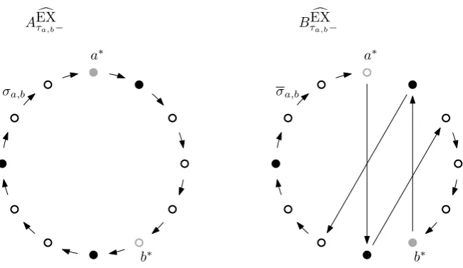
Figure 3 demonstrates the relationship betweenσa,bandσa,bin the simple case where

σa,b is a single cycle. To show that this is a valid coupling, it suffices to show that in case

Figure 3: The left/right image shows the state of the process on edgeea,bat timeτa,b−

in the ‘A’/‘B’ process. Also indicated are the permutationsσa,bandσa,bwhich are to be

applied in case (iii).

bijection between the two permutations. By inspection, the cyclic decomposition ofσa,b

is obtained from that ofσa,b just by exchanging the elementsσa,b(a∗)andσa,b(b∗), and

so both permutations belong to the same conjugacy class. Moreover, there is a bijection between them since

σa,b(a∗) =σa,b(b∗) and σa,b(b∗) =σa,b(a∗),

and soJ1(σa,b) =J1(σa,b)andJ2(σa,b) =J2(σa,b).

Furthermore, it follows from the above analysis that our coupling strategy in case (iii) givesσa,b(a∗) = ˜σa,b(b∗), and furthermore,σa,b( ˆIτa,b−(D)) =σa,b( ˆIτa,b−(D)). Thus in order to complete this proof, we need to show that

P_{[θa,b= 1, J2(σa,b)|σa,b(a}∗_)6=a∗_{},{|ea,b|>4]≥2/25.}

We have

P_{[J1(σa,b)|σa,b(a}∗_)6=a∗_,|ea,b|>4]

=P_[σa,b(a∗_{)∈ {/ a}∗_{, b}∗_{} |σa,b(a}∗_{)∈/ a}∗_,|ea,b|>4]

·P_[σa,b(b∗_{)∈ {/ a}∗_{, b}∗_{} |σa,b(a}∗_{)∈ {/ a}∗_{, b}∗_},|ea,b|>4].

Using parts 2 and 3 of Assumption 1.1) this becomes

P_{[J1(σa,b)|σa,b(a}∗_)6=a∗_,|ea,b|>4]

≥ 4 5

1−P_[σa,b(b∗_{) =b}∗_]−1−P[σa,b(b

∗_{) =b}∗_]

4

≥ 12

25.

Therefore,

P_{[θa,b= 1, J2(σa,b)|σa,b(a}∗_)6=a∗_,|ea,b|>4]

=1

2P[J1(σa,b)|σa,b(a

∗_)6=a∗_{, |e}

a,b|>4]

·P_{[J2(σa,b)|J1(σa,b), σa,b(a}∗_)6=a∗_{, |ea,b|>4]}

≥ 6

25P[J2(σa,b)|J1(σa,b), σa,b(a

∗_)6=a∗_,|e

But conditioned onJ1(σa,b)and{σa,b(a∗)6=a∗,|ea,b| >4}both holding,J2(σa,b)is the

event that two of the positions in ea,b not containing a∗ or b∗ either both contain a

matched particle or are both empty; since|ea,b| ≥5this probability is at least1/3, thanks

to part 2 of Assumption 1.1, and so our proof is complete.

We now present the main result of this section.

Lemma 4.4.There exists κ > 0 such that for any easy hypergraph G, any f and 0< ε <1/2,

TEX(k,f,G)(ε)≤κlog(1/ε)TEX(k−1,f,G)(1/4),

for any3≤k≤ |V|/2if|V|<36and anyk∈ {3,4}if|V| ≥36.

In this section we will make use of this lemma only for the case|V| ≥36, but this result will later be used in its full form when dealing with the case of|V| < 36: see Section 5. The proof uses a coupling argument for two realisations of EX(k, f, G).

Proof. ForU = {u1, . . . , uk}, W = {w1, . . . , wk} ∈ V_k

, let (UtEX)t≥0 and (WtEXf)t≥0 be

two realisations of EX(k, f, G)started fromU andW respectively. We define the two processes on a common probability space, and will show how to couple them in such a way that we can lower-bound the probability thatUEX

κT =WκTEXf for someκ >0to be

determined, whereT :=TEX(k−1,f,G)(1/4). The result will then follow by applying (2.4).

We begin by allowing the two processes to evolve independently up to time10T. Then, for anyS⊂ V_kandt≥0, we have

P_U10EX_T+t∈S−P

h

W10EXfT+t∈S

i =E

h

P_U10EX_T+t∈S|U10EX_T−P

h

W10EXfT+t∈S|W

f EX 10T ii ≤E h

kL[U10EXT+t|U10EXT]− L[W

f

EX 10T+t|W

f

EX 10T]kTV

i

,

where the inequality follows from (2.2). Maximizing overSand again using (2.2) gives

kL[U10EXT+t]− L[W

f

EX

10T+t]kTV ≤E

h

kL[U10EXT+t|U10EXT]− L[W

f

EX 10T+t|W

f

EX 10T]kTV

i

. (4.2)

By the Markov property, for anyA, B ∈ V_k,

kL[U10EXT+t|U10EXT =A]− L[W

f

EX 10T+t|W

f

EX

10T =B]kTV =kL[AEXt ]− L[B

f

EX

t ]kTV

≤Ph_AEX

t 6=B

f

EX

t

i

, (4.3)

for any coupling of(AEX

t )t≥0 and(BtEXf)t≥0, by (2.4), and whereL[·|·]denotes a

condi-tional law.

Recall from Section 2.2 the construction of the permutationItfor eacht≥0. For any

A, B∈ V_k, letaandbbe two uniformly and independently chosen elements ofAandB, respectively. Givena, consider now thek-particle process(Aat)t≥0= (It(a), It(A\{a}))t≥0

which evolves in the same way as the exclusion process begun atA, but with the label of the particle started from positionabeing tracked. Thus(Aa

t)t≥0can be thought of

as something ‘between’ an exclusion process (in which no labels are tracked) and an interchange process (in which all labels are tracked). It’s clear that thek−1particles initially at vertices inA\{a}behave marginally as an exclusion process, while the particle started fromabehaves (again marginally) as a random walk onG. Furthermore, the exclusion process(AEX

t )t≥0can be recovered from(Aat)t≥0simply by ‘forgetting’ which

position is occupied by the ‘special’ particle starting froma, i.e.AEX

t ={It(a), It(A\{a})}.

In a similar manner, for givenband another permutation-valued process( ˜It)t≥0, we also

define the process( ˜Bb

Over the time period[0,10T]we couple the processes(Aat)t≥0and( ˜Btb)t≥0using a

maximal coupling of the(k−1)-particle exclusion processesIt(A\ {a})andI˜t(B\ {b}).

(Recall that a maximal coupling is one which achieves equality in the coupling inequality (2.4). This maximal coupling is actually more than is needed here; we will only be interested in the state of the processes at time10T.) By Proposition 2.2 we have

TEX(k−1,f,G)(1/500)≤

& log 1 500 log 1 2 '

T <10T. (4.4)

Given the choice ofaandb, letFa,bdenote the event that the other(k−1)particles have

coupled by time10T, i.e. Fa,b =I10T(A\ {a}) = ˜I10T(B\ {b}) . Using this maximal

coupling it follows from (4.4) thatP_{[Fa,b] ≥499/500}. Combining this with equations (4.2) and (4.3) we see that for anyK∈N,

kL[U₍₂₀₊EX _K)T]− L[W₍₂₀₊EXf _K)T]kTV

≤ X

A,B∈₍V_k) P

h

U10EXT =A, W10EXfT =B

i

P

h

AEX(10+K)T 6=B(10+EXf K)T

i

= X

A,B∈(Vk)

P_U10EX_{T =A}Ph_W10EXf_{T =B}iPh_AEX

(10+K)T 6=B

f

EX (10+K)T

i

≤ X

A,B∈₍V_k)

P_U10EX_{T =A}P

h

W10EXfT =B

i

·X

a∈A b∈B

1

k2

1−P_{[Fa,b] +}Ph_AEX

(10+K)T 6=B

f

EX

(10+K)T, Fa,b

i

≤ 1 500+

X

A,B∈₍V_k)

P_U10EX_{T =A}P

h

W10EXfT =B

i X

a∈A b∈B

1

k2P

h

AEX(10+K)T 6=B(10+EXf K)T, Fa,b

i

,

(4.5)

where the equality is thanks to the independence ofU andW over[0,10T]. From (4.5) we see that we now need to upper bound the probability that(AEX

t )t≥0and

(BEXf

t )t≥0do not agree by time(10 +K)T, on the eventFa,b. As pointed out above, this

event is equivalent (onFa,b) to thelocationsof thekparticles inAa_(10+K)T andB˜₍₁₀₊b _K)T

not agreeing.

We shall bound this probability by coupling the processes(Aa

10T+t)t≥0and( ˜B10b T+t)t≥0

in the following manner. Recall the Poisson process Λ of rate 2|E| at the start of Section 4.1 with associated edge-choices{en}n∈N, permutations{σn}n∈N, and Bernoulli (1/2)random variables{θn}n∈N(used to thin the events ofΛ). Prior to a timeτ_a,bdefined

below we evolve(Aa

10T+t)t≥0and( ˜B10b T+t)t≥0by applying permutationσn to edgeen(in

both processes) at thenth_{incident time ofΛif and only ifθ}

n= 1, so formally we have for

each0≤t < τa,b,

Aa10T+t= ˆIt I10T(a), I10T(A\ {a})

, B˜10b T+t= ˆIt I˜10T(b),I˜10T(B\ {b})

.

Note that, since we use a common set of innovations over the period[10T,10T+τa,b), on

eventFa,bwe haveD:= ˆIτa,b−(I10T(A\ {a})) = ˆIτa,b−( ˜I10T(B\ {b})); that is, the locations of thek−1unlabelled particles ofAa _andB˜b _{still agree at timeτ}

a,b−. By the Markov

property, on eventFa,b we can thus write

We defineτa,bto be the first time that the ‘special’ particles initially ataandbare in

a common edge which then rings (note this has a slightly different definition fromτa,b

defined in the statement of Lemma 4.3):

τa,b:= inf{t≥0 : ˆIt(I10T(a)),Iˆt( ˜I10T(b))∈eΛ[0,t]}.

Note that the processes( ˆIt(I10T(a)))t≥0and( ˆIt( ˜I10T(b)))t≥0when viewed marginally

behave as independent random walks over the period[0, τa,b), and soτa,b has the same

distribution as the meeting timeMRW_(I

10T(a),I˜10T(b))in (4.1).

To determine how to couple the processes at timeτa,bwe partition the probability

space according to the following four sets (for someK∈N_{which is yet to be determined),}

denotingIˆτa,b−(I10T(a))bya

∗_{for ease of readability:}

Ea,b1 :={τa,b> KT},

Ea,b2 :={τa,b≤KT, σa,b(a∗) =a∗},

Ea,b3 :={τa,b≤KT, σa,b(a∗)6=a∗,|ea,b|>4},

Ea,b4 :={τa,b≤KT, σa,b(a∗)6=a∗,|ea,b| ≤4}.

For the first two cases, we shall not specify the coupling, as it does not matter how we update the processes at timeτa,b. First, for the case ofEa,b1 , we have

X

A,B∈₍V_k)

P_U10EX_{T =A}P

h

W10EXfT =B

i X

a∈A b∈B

1

k2P

h

AEX(10+K)T 6=B

f

EX

(10+K)T, Fa,b, Ea,b1

i

≤ X

A,B∈₍V_k)

P_U10EX_{T =A}Ph_W10EXf_{T =B}i X

a∈A b∈B

1

k2P

Ea,b1

≤max

a,b

P_Ea,b1 _. (4.6)

Second, for the case ofE2

a,b, we have

X

A,B∈₍V_k)

P_U10EX_{T =A}P

h

W10EXfT =B

i X

a∈A b∈B

1

k2P

h

AEX(10+K)T 6=B

f

EX

(10+K)T, Fa,b, Ea,b2

i

≤ X

A,B∈₍V_k)

P_U10EX_{T =A}P

h

W10EXfT =B

i X

a∈A b∈B

1

k2P[σa,b(a

∗_{) =a}∗_]

= X

a,b∈V

1

k2P[σa,b(a

∗_{) =a}∗_]Pa∈UEX 10T

Ph_b∈WEXf

10T

i

≤ k

2

|V|2

X

a,b∈V

1

k2P[σa,b(a

∗_{) =a}∗_{] +kL[(a, b)}RW

10T]−Unif(V2)kTV (4.7)

≤ 1

|V|2

X

a,b∈V

P_[σa,b(a∗_{) =a}∗_{] +} 2

500, (4.8)

where the penultimate inequality uses (2.1) and (2.3) and the last inequality uses (2.5), (4.4) and the contraction principle.

Third, conditioned on the event E3

processes so thatIˆτa,b(I10T(A)) = ˆIτa,b( ˜I10T(B))with probability at least2/25, giving

X

A,B∈(Vk)

P_U10EX_{T =A}P

h

W10EXfT =B

i X

a∈A b∈B

1

k2P

h

AEX(10+K)T 6=B

f

EX

(10+K)T, Fa,b, Ea,b3

i

≤ X

A,B∈₍V_k)

P_U10EX_{T =A}P

h

W10EXfT =B

i X

a∈A b∈B

1

k2

23

25P[σa,b(a

∗_)6=a∗_,|e

a,b|>4]

≤ 2 500 +

23 25|V|2

X

a,b∈V

P_[σa,b(a∗_)6=a∗_,|ea,b|>4], (4.9)

where the last inequality is obtained in the same way as (4.8). Our fourth and final case to consider is E4

a,b: on this event a simple case-by-case

analysis (sketched in Appendix A) shows that as long as there are no other (already matched) particles on edgeea,bat timeτa,b−(i.e.|Iˆτa,b−(I10T(A))∩ea,b|= 1), there exists a bijection between permutationsσa,b and˜σa,bsuch thatσ˜a,b is a permutation with the

same cycle structure asσa,b, and such that with probability at least1/2

σa,b Iˆτa,b−(I10T(a))

= ˜σa,b Iˆτa,b−( ˜I10T(b))

.

That is, in this situation we are able to make the locations of allkparticles ofAEX (10+K)T

andBEXf

(10+K)T agree with probability at least1/2:

Ph_AEX

(10+K)T =B

f

EX

(10+K)T, Fa,b, Ea,b4

i ≥1

2P h

|Iˆτa,b−(I10T(A))∩ea,b|= 1, Fa,b, E

4

a,b

i

.

We use a union bound to control the probability of the complement and writec∗_for

ˆ

Iτa,b−(I10T(c))andb

∗_forIˆ

τa,b−( ˜I10T(b)). We have

X

A,B∈₍V_k)

P_U10EX_{T =A}P

h

W10EXfT =B

i X

a∈A b∈B

1

k2P

h

AEX(10+K)T 6=B(10+EXf K)T, Fa,b, Ea,b4

i

≤ X

A,B∈₍V k)

P_U10EX_{T =A}P

h

W10EXfT =B

i

·X

a∈A b∈B

1 2k2

P_Ea,b4 ₊P

h

|Iˆτa,b−(I10T(A))∩ea,b|>1, a

∗_6=b∗_{, E}4

a,b

i

≤ X

A,B∈₍V_k)

P_U10EX_{T =A}P

h

W10EXfT =B

i

·X

a∈A b∈B

1 2k2



P_Ea,b4 ₊ X

c∈A\{a}

P_c∗_{∈ea,b, c}∗ _6=b∗_{, a}∗_6=b∗_{, Ea,b}4

 

= X

a,b∈V

X

c6=a

1 2k2

 

Ph_E4

a,b

i

k−1 +P

c∗∈ea,b, c∗6=b∗, a∗6=b∗, Ea,b4

 

· X

A⊃{a,c}

B⊃{b}

P_U10EX_{T =A}Ph_W10EXf_{T =B}i_. (4.10)

gives the following upper bound for (4.10):

2 500+

k2_(k−1)

|V|2_{(|V| −1)}

X

a,b∈V

X

c6=a

1 2k2

 P h E4 a,b i

k−1 +P

c∗∈ea,b, c∗6=b∗, a∗6=b∗, Ea,b4

_

≤ 2 500+

1 2|V|2

X

a,b∈V

P_Ea,b4

+ k−1 2|V|2_{(|V| −1)}

X

a,b∈V

X

c6=a

P_c∗_{∈ea,b, c}∗_6=b∗_{, a}∗_6=b∗_{, Ea,b}4

≤ 2 500+

1 2|V|2

X

a,b∈V

P_Ea,b4 ₊ k−1 |V|2_{(|V| −1)}

X

a,b∈V

P_Ea,b4 _,

since, on the event E4

a,b, the size of edge ea,b is at most four and so on the event

{a∗_6=b∗_{}for any choice ofe}

a,bthere are only two possibilities for the value ofc(since

c∗_{∈ {/ a}∗_{, b}∗_{} ⊂e}

a,b}). This gives

X

A,B∈₍V_k)

P_U10EX_{T =A}P

h

W10EXfT =B

i X

a∈A b∈B

1

k2P

h

AEX_(10+K)T 6=B₍₁₀₊EXf _K)T, Fa,b, Ea,b4

i

≤ 2 500 +

1 |V|2

1 2+

k−1 |V| −1

X

a,b∈V

P_[σa,b(a∗_)6=a∗_{,|ea,b| ≤4].} (4.11)

We now combine the bounds in (4.5), (4.6), (4.8), (4.9) and (4.11) to see that

kL[U₍₂₀₊EX _K)T]− L[W₍₂₀₊EXf _K)T]kTV≤

7

500+ maxa,b

P_Ea,b1 ₊ 1 |V|2

X

a,b

P_[σa,b(a∗_{) =a}∗_]

+ 1 |V|2max

23 25,

1 2 +

k−1 |V| −1

X

a,b

P_[σa,b(a∗_)6=a∗_].

By assumption,k≤ |V|/2if|V|<36andk∈ {3,4}if|V| ≥36, and so

max 23 25, 1 2+

k−1 |V| −1

≤ 33

34

for all possible combinations ofkand|V|being considered here. Combining this bound with that in Assumption 1.1, we obtain:

kL[U(20+EX K)T]− L[W

f

EX

(20+K)T]kTV≤ 7

500+ maxa,b

P_Ea,b1 ₊1 5

1 + 4·33 34

.

But since τa,b has the same distribution as MRW(I10T(a),I˜10T(b)), and G is an easy

hypergraph,

max

a,b

P_Ea,b1 _{= max}

a,b

P_{[τa,b > KT]≤max}

a,b

P_MRW_{(a, b)> KT≤} 1 1000

providedK≥1010_{. Therefore,}

kL[U10EX11_T]− L[W₁₀EXf11_T]kTV≤

8 500+

1 5

1 + 4· 33 34

< 497

500.

Finally, by submultiplicativity of the function

¯

d(t) := max

U,W∈₍V_k)kL[U

EX

(see e.g. Lemma 4.12 of [10]), we deduce that

kL[U10EX14_log(1/ε)T]− L[W₁₀EXf14_log(1/ε)T]kTV <

₄₉₇

500

1000 log(1/ε)

< ε ,

and so the statement of Lemma 4.4 is proved upon takingκ= 1014_.

Proof of Lemma 1.10 for easy hypergraphs. We simply apply Lemma 4.4 for the case |V| ≥36twice, first withk= 4and then withk= 3(and takeε= 1/4both times). We deduce that

TEX(4,f,G)(1/4)≤κ2(log 4)2TEX(2,f,G)(1/4),

and so it suffices to takeλ=κ2_{(log 4)}2_.

4.2 From 4-particle exclusion to 2-particle exclusion: non-easy hypergraphs

We begin with a result showing that for non-easy hypergraphs the average meeting time for two independent random walkers is unlikely to be quick. Intuitively, this follows from the following observations. We know there exists a pair of vertices such that random walkers started from these two states likely take a long time to meet. If we look at where these two walkers are at time of orderTRW(f,G)(1/4), they will be close to

uniform. Hence, starting random walkers from a uniform pair we see that they will likely still take a long time to meet. The proofs of Lemmas 4.5 and 4.6, and of Proposition 4.7 are (somewhat technical) extensions of corresponding results of [15], and can be found in Appendix B.

Lemma 4.5.For every non-easy hypergraph we have

X

u∈V2

P_MRW₍u)≤20T

|V|2 ≤

1 1000.

Given a k-tuplez∈ (V)k, we once again writeO(z) := {z(1), . . . ,z(k)}for the

(un-ordered) set of coordinates ofz. Forx∈V4_{, letx}RW

t be a realisation of RW(4, f, G)with xRW₀ =x. Denote byΛ1_,Λ2_,Λ3_,Λ4_{the (independent) Poisson processes used to generate}

the edge-ringing times for the four random walkers, and let{e1

n}n∈N,{e2_n}_n∈N,{e3_n}_n∈N, {e4

n}n∈N be the four sequences of edge-choices (all as in Section 2.2).

We now defineM¯RW_{(O(x))to be the first timeany twoofx}RW

t (1),xRWt (2),xRWt (3), xRW_t (4)first arrive onto the same edge which then rings for one of them. Formally,

¯

MRW(O(x)) := infnt≥0 : ∃1≤i < j≤4, e∈ {eiΛi_[0,t], e

j

Λj_[0,t]}

withxRW_t− (i),xRW_t− (j)∈eo.

Lemma 4.6.Letx∈(V)4. Then for anyε∈(0,1),

P_M¯RW₍O(x)EX20T)≤20T

≤12(ε+ε−12−20) + 25(1 +ε) X

u∈V2

P_MRW₍u)≤20T

|V|2

Next, we provide a bound which relates the total-variation distance between two 4-particle exclusion processes to the probability that any two of four independent walkers have ‘met’.

Proposition 4.7.For anyx∈(V)4ands≥0:

Lemma 4.8.For every non-easy hypergraphGand any two realisations of EX(4, f, G), denoted{AEX

t }and{BtEX}, we have

kL[AEX40T]− L[B40EXT]kTV≤P

_¯

MRW(AEX20T)≤20T

+P_M¯RW_(B20EX_{T)≤20T+ 2}−18_.

Proof. By Proposition 4.7 and the triangle inequality for total-variation, for anyu,v∈ (V)4,

kL[O(u)EX20T]− L[O(v)EX20T]kTV≤P

_¯

MRW(O(u))≤20T+P_M¯RW₍O(v))≤20T

+kL[O(uRW_20T)]− L[O(vRW_20T)]kTV. (4.12)

An identical argument to that used for equation (4.2) tells us that

kL[AEX

40T]− L[B40EXT]kTV≤E

kL[AEX

40T|AEX20T]− L[B40EXT|B20EXT]kTV

.

Applying the inequality in (4.12), with anyu,vsatisfyingO(u) =AEX

20T andO(v) =BEX20T,

gives

kL[AEX

40T]− L[B40EXT]kTV ≤E

P_M¯RW_(AEX

20T)≤20T|AEX20T

+EP_M¯RW_(B20EX_T)≤20T|B20EX_T

+ sup u,v∈(V)4

kL[uRW_20T]− L[vRW_20T]kTV.

Using Proposition 2.3 and the contraction principle for the third term on the right-hand side gives the desired result.

We are now ready to prove the main result of this subsection.

Proof of Lemma 1.10 for non-easy hypergraphs. We in fact show that for any two reali-sations of EX(4, f, G), denoted{AEX

t }and{BtEX}, we have

kL[AEX40T]− L[B40EXT]kTV≤1/4.

Combining Lemmas 4.6 and 4.8 we have that for everyε∈(0,1),

kL[AEX40T]− L[B40EXT]kTV≤24(ε+ε−12−20) + 50(1 +ε)

X

u∈V2

P_MRW₍u)≤20T

|V|2 + 2 −18_.

Now by Lemma 4.5, this becomes

kL[AEX

40T]− L[BEX40T]kTV≤24(ε+ε−12−20) +

50(1 +ε) 1000 + 2

−18_.

Settingε= 10−3_{completes the proof.}

5

From

k

_{-particle exclusion to 2-particle exclusion for small}

_|

V

_|

We now prove Lemma 1.7. We begin by showing that any hypergraphGwith|V|<36 satisfies

sup y∈V2

P_MRW₍y)>1010_T

RW(f,G)(1/4)

≤1/1000, (5.1)

i.e. the hypergraphGiseasy. Indeed, by Proposition 2.4, for anyt≥2TRW(f,G)(ε),

sup y∈V2

P_MRW₍y)< t≥(1−2ε)

2

|V| ≥

(1−2ε)2

and so

sup y∈V2

P_MRW₍y)>2000TRW(f,G)(1/4)

≤1/1000,

which certainly implies (5.1). SinceGis easy, we can apply Lemma 4.4 multiple times to deduce that

TEX(k,f,G)(ε)≤κk−2(log(1/4))k−3log(1/ε)TEX(2,f,G)(1/4).

However, since|V|<36andk≤ |V|/2 the statement of the proof is complete taking

C=κ15_(log(1/4))14_.

6

The chameleon process

Our aim in this section is to construct a continuous-time Markov process which satisfies the properties of(Mt)t≥0outlined in Lemma 3.1. We will call this process the

chameleon process. In Section 7 we will prove Lemma 3.1 by demonstrating that the chameleon process does indeed have the desired properties.

The chameleon process was originally constructed (in a different form but to serve a similar purpose) by Morris ([14]), and then adapted by Oliveira ([15]) to analyse the mixing time of thek-particle interchange process on a graph (as opposed to on a hypergraph, as we consider here). It is built on top of an underlying interchange process, with the aim of helping to describe the distribution of the location of thekth particle in this process, conditional on the locations of thek−1other particles.

Unlike in ak-particle interchange process which always haskparticles, the chameleon process has|V|particles (one at each vertex), although not all particles are distinguish-able from each other. In addition, each particle has an associatedcolour: one of black, red, pink and white (which correspond to the processes zC_t, Rt, Pt, Wt respectively,

appearing in the statement of Lemma 3.1). The movement of particles in the chameleon process follows that of the underlying interchange process in the sense that the locations of particles in both processes are updated using the same functionsIas described in the graphical construction of Section 2.2. At some of the updates of the underlying interchange process we will colour some of the red and white particles pink (precisely when this happens is rather involved and is the subject of Section 6.2). To provide some insight into when these pinkening events occur, consider the chameleon process of [15]: here, if the vertices at the endpoints of a ringing edge are occupied by a red and a white particle then both of these particles are recoloured pink. In the lazy version of the interchange process on a graph (in which nothing happens with probability 1/2 when an edge rings), when an edge rings with endpoints occupied by a red and a white particle, with probability 1/2 they switch places and with probability 1/2 they do not move. Colouring both particles pink (which should be viewed as half red, half white) encodes the fact that at either vertex just after the edge rings we may have a red particle or a white particle, and these are equally likely.

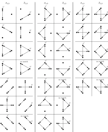
the particles on that edge. To decide which particles to pinken, we construct a twin permutationσ˜with the property that the trajectories of all black particles in the edge are identical under both permutations (a required property – see part 1 of Lemma 3.1), and such that, viewed marginally, the distribution ofσ˜ agrees with that ofσ. We then look for verticesvsuch that underσa red particle is moved tovand underσ˜ a white particle is moved tov; a certain subset of these particles will be pinkened. The simplest example to consider is that of an edge of size 3 which contains one red, one white and one black particle, and for whichfeis constant onSe. In this case, it is straightforward

to construct a twin permutation with these required properties, and the construction is sketched in Figure 4.

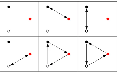
Figure 4: Consider an edge of size 3, containing one red, one white and one black particle, and for whichfeis constant onSe. The six possible permutations are sketched

here: in this example the twin of any given permutationσcould be taken to be the permutation immediately above/belowσ. Note that in each case the black particle follows the same trajectory under bothσand its twin; moreover, ifσmoves a red/white particle to a vertexv, then its twin moves a white/red particle tov. In this simple example we could therefore pinken the red and white particles, no matter whichσis chosen.

Although this example demonstrates one possibility for generating twin permutations with our desired properties, this isvery particular to the situation in whichfeis constant

onSe– a much stronger condition than we are imposing in Assumption 1.1. In general,

we shall make use of the fact thatfeis constant on conjugacy classes to construct a twin

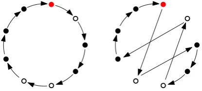
permutationσ˜ with thesame cycle structure asσ. (Note that the twin permutations constructed in Figure 4 do not have the same cycle structure asσ, and so we shall need to come up with an alternative method of pinkening, even when considering edges of size 3.) Figure 5 gives an indication of howσ˜will be produced from knowledge ofσand the particle colours in the case ofσbeing a single cycle: by modifying the trajectories of four particular particles we are able to ensure that not only doesσ˜have the same cycle structure asσ, but that the trajectories of all black particles in the edge are identical under both permutations. It is for this reason (i.e. needing to know the colours of four particular particles) that we are able to relate the mixing time ofkparticles to that of just four particles in Lemma 1.8.