This is a repository copy of Crime at Places and Spatial Concentrations: Exploring the Spatial Stability of Property Crime in Vancouver BC, 2003–2013.
White Rose Research Online URL for this paper: http://eprints.whiterose.ac.uk/98995/
Version: Accepted Version
Article:
Andresen, MA, Linning, SJ and Malleson, N orcid.org/0000-0002-6977-0615 (2017) Crime at Places and Spatial Concentrations: Exploring the Spatial Stability of Property Crime in Vancouver BC, 2003–2013. Journal of Quantitative Criminology, 33 (2). pp. 255-275. ISSN 0748-4518
https://doi.org/10.1007/s10940-016-9295-8
[email protected] https://eprints.whiterose.ac.uk/ Reuse
Unless indicated otherwise, fulltext items are protected by copyright with all rights reserved. The copyright exception in section 29 of the Copyright, Designs and Patents Act 1988 allows the making of a single copy solely for the purpose of non-commercial research or private study within the limits of fair dealing. The publisher or other rights-holder may allow further reproduction and re-use of this version - refer to the White Rose Research Online record for this item. Where records identify the publisher as the copyright holder, users can verify any specific terms of use on the publisher’s website.
Takedown
If you consider content in White Rose Research Online to be in breach of UK law, please notify us by
Crime at places and spatial concentrations: Exploring the
spatial stability of property crime in Vancouver BC,
2003-2013
Martin A. Andresen1, Shannon J. Linning2, and Nick Malleson3
Objectives. Investigate the spatial concentrations and spatial stability of criminal event data at the micro-spatial unit of analysis in Vancouver, British Columbia.
Methods. Geo-referenced crime data, 2003 2013, representing four property crime types (commercial burglary, mischief, theft from vehicle, theft of vehicle) are analyzed considering crime
concentrations at the street segment and street intersection level as well as through the use of a
nonparametric spatial point pattern test that identifies the stability in spatial point patterns in
pairwise and longitudinal contexts.
Results. Property crime in Vancouver is highly concentrated in a small percentage of street segments and intersections, as few as 5 percent of street segments and intersections in 2013 depending on the
crime type. The spatial point pattern test shows that spatial stability is almost always present when
considering all street segments and intersections. However, when only considering the street
segments and intersections that have crime, spatial stability is only present in recent years for
pairwise comparisons and moderately stable in the longitudinal tests .
Conclusions. Despite the crime drop that has occurred in Vancouver, there is still spatial stability present over time at levels suitable for theoretical development. However, caution must be taken
when developing initiatives for situational crime prevention.
Keywords: crime at places; spatial stability; spatial point pattern test
Suggested running head: Crime at places and spatial concentrations
1 Institute for Canadian Urban Research studies and School of Criminology, Simon
Fraser University, 8888 University Drive, Burnaby BC, V5A 1S6. Email: [email protected]
2 Institute for Canadian Urban Research studies, Simon Fraser University, 8888 University Drive,
Burnaby BC, V5A 1S6; School of Criminal Justice, University of Cincinnati, P.O. Box 210389, 665 Dyer Hall, Cincinnati, OH 45221-0389. Email: [email protected]
3 School of Geography, University of Leeds, West Yorkshire, LS2 9JT, United Kingdom. Email:
1. INTRODUCTION
The spatial stability of crime patterns is important for the development of theory
and the application of policy. If spatial stability is not present, all data analyses are
literally historical without contemporary relevance and cannot be used in a
meaningful way to test/refine/develop theory or make applicable crime prevention
policy.
Research in spatial criminology over the past 25 years has shown that crime
is incredibly concentrated, most often having 50 percent of criminal activity
accounted for in 5 percent of micro-places, or street segments (Sherman et al., 1989;
Weisburd & Amram, 2014). Though this high degree of crime concentration implies
that spatial stability is present, this may not be the case; rather, crime may be highly
concentrated but there still may be enough spatial shifting in the other 50 percent of
crime to cause problems for theory and policy.
As reviewed below, the body of research regarding crime at places and
spatial concentrations of crime is growing, but this literature is still relatively new
and early in its development (Weisburd, 2015). Though research that investigates
these phenomena in different places and at different times is important (one of the
contributions of this paper), there are unanswered questions that must be
investigated to advance the crime at places literature. For example, what is the
importance of the spatial stability of crime patterns? There is indirect evidence for
the presence of spatial stability through the use of traditional trajectory analysis,
of any given city is stable with regard to its crime patterns what can the lack of
stability in the small percentage of that city tell us? Only when spatial stability is
directly measured can such investigations be considered. Also, is the law of crime
concentration at places just a manifestation of the concentration of human
concentrations, in general (Weisburd, 2015)? If this is the case, we should find
greater concentrations of crime where we know there are greater concentrations of
human activity.
In this paper we investigate the presence of spatial stability in municipal
level crime patterns in order to begin to fill these gaps in the crime and place
literature. We use an open source crime data set with four crime types (commercial
burglary, mischief4, theft from vehicle, and theft of vehicle) and an open source
spatial point pattern test that allows for the identification of similarity in spatial
point patterns: we compare the similarity of spatial point patterns over time within
each crime type. We find that despite the significant crime drop that has occurred in
this municipality, a common phenomenon around the world over the past 25 years
(Farrell et al., 2011, 2015; Tseloni et al., 2010), spatial patterns of crime and
concentrations of crime have remained relatively stable. The importance of these
results is discussed in the context of theoretical development and crime prevention
policy.
4 Mischief most often represents some form of property damage or graffiti, but may also include
disorder. This crime type is also the most sensitive to police reporting and patrol activities and
2. SPATIAL STABILITY: ITS IMPORTANCE AND RECENT EVIDENCE
Spatial stability, sometimes referred to as ecological stability, is a concept that is
implicitly assumed when considering the relevance of spatial analyses of crime. This
is particularly the case when researchers analyze one year of data, or average a
small number of years of data. If the spatial patterns do not have spatial stability,
then it is impossible to make predictions with regard to crime levels at other times
or in other places. Without spatial stability, research only tells one about historical
relationships.
The importance of spatial stability was recognized in the context of social
disorganization theory. Shaw et al. (1929) and Shaw and McKay (1931, 1942, 1969)
stated that neighborhoods maintained their relative rankings with regard to
juvenile delinquency (spatial stability) despite the changes in ethnic composition
over time. These researchers were able to make this claim because they had data
that spanned many years. However, a lot of the research in social disorganization
theory that followed did not. Because of the changing nature of cities through the
process of gentrification (Lees et al., 2007), the assumption of spatial stability was
difficult to justify and led to social disorganization falling out of favor in
criminological research (Bursik, 1988). It is important to note spatial patterns may
be persistent despite changes in the urban environment, this assumption could just
not be tested. But does a lack of spatial stability at the neighborhood level
correspond to a lack of spatial stability at micro-places? This is an important
question within the crime and place literature, to test the law of crime concentration
Many years passed before a data set covering an entire city and multiple
years would emerge again that could test the assumption of spatial stability. In a
longitudinal study of crime patterns in Seattle, Washington, Weisburd et al. (2004)
investigated the stability of crime concentrations at the street block level of analysis.
Over a 14-year period, they found that one-half of the crime in Seattle occurs in 4-5
percent of the street blocks and that all crime took place in approximately 50
percent of the street segments. In order to investigate the spatial stability of crime
patterns, Weisburd et al. (2004) used trajectory analysis at the street segment level
and found that the overall majority of all trajectories generated remained relatively
stable over their 14-year period. Moreover, they found that the changing crime rate
trends (decreasing over time) were accounted for by only a small percentage of the
street segments in Seattle.
Weisburd et al. (2009) and Groff et al. (2010) replicated the Seattle study but
in specific contexts. Weisburd et al. (2009) found that juvenile crime was spatially
concentrated to a greater degree than all crime analyzed by Weisburd et al. (2004):
less than one percent of street segments accounted for one-half of the juvenile
criminal incidents in Seattle and all crime was attributed to 3-5 percent of street
blocks over a 14-year period. Groff et al. (2010) found strong evidence for spatial
stability over a 16-year study period and found that different trajectories tended to
be spatially close to one another. This is not evidence counter to spatial stability, but
shows the importance of micro-spatial units of analysis.
In a 29-year longitudinal study in robberies in Boston, Massachusetts, Braga
between 1980 and 2008, and one-half of robberies in Boston occurred in 8.1 percent
of street blocks during that same time period remarkable stability for such a long
time period. In their temporal analyses, Braga et al. (2011) found that chronic street
segments remained chronic over time, providing strong evidence for spatial
stability.
In an analysis of three years of data spanning 10 years (1991, 1996, and
2001), Andresen and Malleson (2011) were the first to explore multiple crime types ,
individually, for the same location over time. Their analyses of assault, burglary,
robbery, sexual assault, theft, theft of vehicle, and theft from vehicle in Vancouver,
British Columbia at three levels of analysis (census tracts, dissemination areas, and
street segments) found that one-half of all crime could be accounted for by 1-8
percent of street segments. Moreover, approximately one-half of all street blocks in
Vancouver experienced none of the crime types with strong evidence that spatial
crime patterns remained relatively stable throughout the years of data examined.
Most recently, Curman et al. (2015) undertook an independent replication of
Weisburd et al. (2004) over a 16-year time period in Vancouver, British Columbia.
In their analyses of crime, 1991 2006, Curman et al. (2015) found very similar
results to that of Weisburd and colleagues: approximately 40 percent of Vancouver
was without any crime reported to the police and the vast majority of trajectories
were classified as stable or with very little change over time.
Despite the strengths within all these studies, they are not without their
limitations. First, aside from Braga et al. (2011), these more recent investigations of
intersections. This is particularly problematic for Curman et al. (2015) because 25
percent of the crime data had to be excluded from their study. Such a large
proportion of data could change spatial patterns according to Weisburd (2015),
crime at intersections can be as low as 0 percent, but as high as 33 percent. Second,
as evident in the actual trajectories shown in Weisburd et al. (2004) and Curman et
al. (2015), though trajectories may be stable from a statistical perspective they may
still be increasing or decreasing by a small degree. Consequently, over longer time
periods it is still possible that actual spatial patterns are changing in meaningful
ways the spatial trajectories may actually be different. The exception to this is
Andresen and Malleson (2011), but they restricted their analyses to three individual
years and only considered pairwise comparisons.
In this paper, as stated above, we investigate the spatial stability of crime
patterns for Vancouver, British Columbia considering four property crime types. We
employ a spatial point pattern test that allows for two types of tests for spatial
stability. First, year-to-year comparisons can be undertaken such that spatial
stability can be compared for pairwise successive years as well as pairwise
comparisons over longer time spans, 2003 to 2013, for example. Second, a
longitudinal version of this spatial point pattern test that considers all years under
analysis for the consideration of spatial stability, the spatial trajectory. This allows
for a test of spatial stability that is more specific than previous research.
This more direct test of spatial stability allows for better information
regarding the degree of stability and to know the degree of instability in spatial
activities (commercial land use and mixed land use for the presence of commercial
burglary) and more ubiquitous human activities (the presence of vehicles and their
associates thefts: theft of and theft from vehicle) we can begin to know if the law of
crime concentration at places is a particular manifestation of the concentrations of
human activities, more generally.
3. DATA AND METHODS
The City of Vancouver is contained within Metro Vancouver, collectively the third
largest metropolitan area in Canada. The Vancouver Census Metropolitan Area
(CMA) is the largest metropolitan area in western Canada, with a population of just
over 2.3 million people. Since 1991, the Vancouver CMA has seen significant
population growth. Most often, this population growth has been linked to the 1986
World Exposition on Transportation and Communication. After this time, the
Vancouver CMA has seen a lot of international investment and subsequent
development. The World Exposition in 1986 brought worldwide attention to the
Vancouver CMA that has only increased because of the relatively recent 2010
Winter Olympics held in this area.
With regard to crime, the Vancouver CMA has the highest level of crime rates
among the three largest metropolitan areas in Canada: 6897 criminal code offences
per 100 000 persons in 2013, more than double the rate in Toronto (2941 per 100
000 persons) and 70 percent greater than the rate in Montreal (4072 per 100 000
persons); the same ranking was present for the violent crime rate in 2013 for
Montreal (903 per 100 000); and, similarly, for property crime in 2013 for
Vancouver (4642 per 100 000 persons), Toronto (1936 per 100 000 persons), and
Montreal (2657 per 100 000). However, it should be noted that with the
international crime drop that began in the early 1990s, the reported differences in
crime rates has decreased in recent years (Boyce et al., 2014; Kong, 1997; Savoie,
2002; Silver, 2007; Wallace, 2003, 2004). Overall, the crime drop that these CMAs
have been of a large magnitude over the study period, 2003 2013: 47 percent
(Vancouver), 42 percent (Toronto), and 35 percent (Montreal). Needless to say, an
investigation into the spatial stability of these crime patterns is in order with this
substantial drop in crime for Vancouver.
3.1. Crime Data and Spatial Units of Analysis
The crime data for Vancouver are police incident data that were retrieved from the
Vancouver Open Data Catalogue.5 These data contain information pertaining to
location and month of occurrence of four crime types over an 11 year period,
2003-2013. The crime types include: commercial break and enter, mischief, theft from
vehicle and theft of vehicle. Though this is a more restricted data set for Vancouver
than used in previous analyses with regard to crime types, these data were the most
current available crime data at the time of data gathering, whereas previous
research using Vancouver data is almost a decade old with its most recent data
point. As such, we chose to conduct a more temporally relevant analysis rather than
attempting to obtain access to the older data for Vancouver.
The nature of the geographic locations provided with these data is the street
intersection or the 100-block6; no specific addresses are provided because these are
open data. The street intersections are easily geocoded, but these data are
problematic in their raw form for geocoding the street addresses. For example, the
address 123 Main Street would be provided as 1xx Main Street. Because of this, and
the need to geocode the data to a street network for subsequent analysis, a random
number generator was used to create a set of numbers ranging from 1 to 99. This
number replaced xx in the original data file. An obvious limitation of these data
and this approach for geocoding is that no inference can be made at the specific
location geocoded for each criminal event. However, as discussed below, all of our
analyses are undertaken at the street block level so there are no issues in regard to
the ecological fallacy and inappropriate inference. With the data recoded, the
geocoding hit rate percentages ranged from 96.3 to 97.1 percent for all four crime
types and all 11 years. This is well above the minimum acceptable hit rate of 85
percent set by Ratcliffe (2004).
The spatial units of analysis for this research, as mentioned above, are street
segment, or 100-blocks, and street intersections. In Vancouver, there are 11,730
street segments. Because of the presence of street intersections in our data and a
desire to retain as much of these data as possible to avoid spatial bias, street
intersections were created using the street segment file. A buffer was set around the
street segments in order to create overlap of the street segments 7 meters was
6 The 100-block is both sides of the street in between two intersections, the same definition for the
found to be sufficient. This overlap was then used to create unique polygons
representing intersections. The resulting total number of spatial units of analysis is
18,445: 6715 street intersections and 11,730 street segments.
In the crime and place literature, criminal events occurring at street
intersections range from 0 to 33 percent (Weisburd, 2015). In the early years of our
data, 2003 2005, criminal events at street intersections comprised of 4 6 percent
of the data. However, in the latter years of the data set, criminal events at street
intersections comprised of 10 12 percent of the data. It is important to note that
these criminal events should not be considered as actually occurring within the
street intersections. Rather, the street intersection is considered to be a better
spatial reporting location to the officer than a street address: a vehicle (stolen or
having property stolen from it) that is parked at the intersection. In fact, there are
even some commercial burglaries that occur at intersections Upon inspection of
these locations, these are locations at which street vendors commonly operate. As
such, these commercial burglaries are burglaries with the street vendor stand as the
target. Given the notable percentage of criminal events in our data and the fact that
these locations are not at random (the street intersections appear in a rather
systematic manner), they should be included in the analysis in order to avoid spatial
bias (Ratcliffe, 2004).
3.2. Spatial Point Pattern Test
In order to assess the spatial stability of crime patterns in Vancouver, 2003 2013, a
statistically significant. One obvious methodology, as outlined above, is trajectory
analysis. This technique allows for the identification of different trajectories for
street segments and intersections. Therefore, if the vast majority of the trajectories
are stable one can assume that the crime patterns are spatially stable. But this is an
assumption. However, there is another test that allows for the identification of
stability of spatial patterns, when considering multiple points in time. The spatial
point pattern test developed by Andresen (2009) can be used to identify spatial
stability through the identification of similarity between multiple spatial point
pattern datasets. To date, this test has been used in a variety of contexts. The initial
application of the test was an investigation of the similarity of spatial patterns
across crime types (Andresen, 2009), but the test has also been used to investigate:
changing patterns of international trade (Andresen, 2010), the stability of crime
patterns (Andresen and Malleson, 2011), the spatial impact of the aggregation of
crime types (Andresen and Linning, 2012), the spatial dimension of the seasonality
of crime (Andresen and Malleson, 2013a; Linning, 2015), the impact of modifiable
areal units on spatial patterns (Andresen and Malleson, 2013b ), the role of local
analysis in the investigation of crime displacement (Andresen and Malleson, 2014),
and the comparison of open source crime data and actual police data (Tompson et
al., 2015).
The spatial point pattern test is summarized as follows, initially considering a
pairwise test for simplicity. The first step is to identify one point-based data set as
the base (2003 mischief, for example) and calculate the percentage of points within
example); second, the other point-based data set is deemed the test data (2013
mischief, for example), and randomly sampled with replacement for 85 percent of
the test data (this allows for the calculation of the percentage of points within each
spatial unit under analysis and 85 percent is based on the research by Ratcliffe
(2004)); third, repeat this sampling process 200 times;7 fourth, calculate the 200
percentages, rank them, and remove the top and bottom 2.5 percent to generate a
95 percent confidence interval; fifth, if the value within a spatial unit of analysis for
the base data set (2003 mischief, for example) is within the 95 percent confidence
interval, that spatial unit of analysis is similar; and sixth, repeat this last step for all
spatial units of analysis. Further details are available in Andresen (2009) and
Andresen and Malleson (2011).
A global statistic can be calculated using the output from the statistical
testing, outlined above. This statistic measures the degree of similarity between the
two datasets, the similarity index, S. The similarity index ranges between 0 (no
similarity) and 1 (perfect similarity), calculated as follows:
(1)
where is equal 1 if the pattern of two datasets are similar and 0 otherwise (this
similarity is defined by step 5 described above), and n is the number of areas.
7Often in the spatial analysis literature 50 repeated samples are used (Davis & Keller, 1997).
However, early research on Monte Carlo experiments by statisticians showed that as few as 20
repeated samples would provide good results (Hope, 1968). We use a 200 repeated random sample
for the purposes of being conservative and to provide convenient cut-off values for the confidence
Consequently, the similarity index measures the percentage of areas that share a
similar pattern. In the literature that has used this spatial point pattern test, a rule of
thumb has emerged to indicate the point at which S indicates similarity. This rule of
thumb is similar to rules of thumb relating to multicollinearity in a regression
context. The variance inflation factor (VIF) is often used as a regression diagnostic
to indicate levels of multicollinearity that can cause issues with inference, most
often when the VIF is in the range of 5 to 10 (O Brien, 2007). Though the VIF can be
calculated with many explanatory variables, the range of 5 to 10 is equivalent to a
bivariate correlation of 0.80 to 0.90. As such, an S-Index value of 0.80 is considered
to represent two spatial point patterns that are similar. Though not practical with
over 18,000 spatial units under analysis, it is important to note that the results of
this test can be mapped showing the local level results, (Andresen, 2009). We
used the graphical user interface (GUI) that was developed for the application of this
spatial point pattern test that can perform the pairwise version of this spatial point
pattern test.8
The nature of the spatial point pattern test, as described and executed in the
GUI, undertakes pairwise comparisons of spatial point patterns. Though instructive,
as shown below, such pairwise tests are limited with regard to the investigation of
spatial stability. For example, subsequent pairwise comparisons (2003 -2004,
2003-2005, 2003-2006, and so on) may indicate high degrees of similarity, S >= 0.90.
However, if the 10 percent of non-similar spatial units changes with every pairwise
comparison, by the time 10 years have passed spatial similarity will actually be
quite low.
In order to address this limitation of previous research using this spatial
point pattern test, we contribute to this literature through an expansion/extension
of Andresen s spatial point pattern test by making it longitudinal in order to
properly assess the stability of spatial trajectories. This is done by allowing for
multiple test data sets )n the current analysis is still considered the base
data set. However, all other subsequent years are independently considered test
data sets, repeatedly randomly sampled, and used to calculate confidence intervals
for statistical testing a confidence interval is generated for each year to be
compared to the base data set.
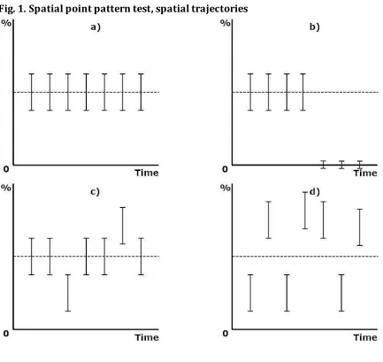
The possible outcomes from this longitudinal version of the spatial point
pattern test are illustrated in Fig. 1. In Fig 1, each dashed horizontal line represents
the base year percentage. Each of the vertical lines represents the confidence
interval for each of the test data sets, years in the current analysis. Fig. 1 only shows
8 years of data (1 base year and 7 test years), so it is for illustrative p urposes, not
representing all of the years in the current analysis.
<Insert Fig. 1 About Here>
The first possibility of a completely stable spatial trajectory is shown in Fig.
1a. As stated above, the dashed horizontal line represents the percentage of po ints
in the base data set that are assigned to each spatial unit (street segment or
intersection in the current analysis). By definition, this percentage is considered
any deviations in the spatial patterns are measured for each year. The vertical lines
represent the confidence intervals for each subsequent test year that are generated
from the repeated sampling procedure. In each case within Fig. 1a, the base data
percentage is within the confidence intervals so this particular spatial unit would be
considered having a stable spatial trajectory. It is important to note here that a
stable spatial trajectory is not necessarily the same as a stable trajectory as defined
in other crime and place research (Curman et al., 2015; Weisburd et al., 2004). In the
current context, a stable spatial trajectory is one in which a spatial unit of analysis
has the same percentage of points; as such, the volume of crime may be going up or
down but it is changing proportionately.
Fig 1b shows the situation of crime no longer occurring on a particular
spatial unit the latter confidence intervals are only present on the x-axis, and made
smaller, for illustrative purposes. In this particular case, crime has a stable spatial
trajectory for the first few years and then crime disappears; a new level of stability
is found in this case. This situation becomes important below. A volatile spatial
trajectory is represented in Fig. 1c. In this scenario, sometimes the confidence
intervals for the test years include the base year percentage and other times they do
not. And finally, Fig. 1d shows no stability in the spatial pattern: after 2003 the
percentage of points has completely changed.
From these possibilities, three new S-Indices are calculated. The first, SAbsolute,
represents Fig 1a: the percentage of spatial units of analysis (street segments and
street intersections) that exhibit total spatial stability. The second, SZero, is calculated
pattern in Fig. 1b to also be a stable spatial trajectory. Of course this is not true in an
absolute sense, hence the names of the first two indices, but it represents the
situation when crime stops occurring in a place altogether it found a new stability
And third, SSum, is an index that represents all of the times when the base and test
values are similar most of the time As such this index does not punish a spatial
unit of analysis and classify it as dissimilar when it is only dissimilar one or two
times over a longer study period. This situation is represented in Fig. 1c with 5 of
the 7 years being classified as similar: 5/7 = 0.71. So, such a spatial unit of analysis is
not stable in an absolute sense, but is generally stable over longer periods of time.
These three indices each also take 2 forms. The first considers all street
segments and street intersections whether they have crime or not. This is the closest
similarity to the previous trajectory modeling in crime and place. The places that
always have zero crime would be classified as low crime and stable trajectories. The
second only considers street segments and intersections that actually have crime.
This form of the index can identify the degree of spatial stability where crime
actually occurs without being influenced by the places that never have criminal
activity. In order to make these calculations the non-zero street segments and street
intersections were defined as any street segment of intersection that had at least
one crime over the study period; for consistency, this same definition was used for
the pairwise comparisons as well. Consequently, when two or more point data sets
are compared, the set of street segments and intersections is complete such that all
two forms of their calculations, each crime type will have six new S-Index values to
be considered for their longitudinal spatial trajectories.
4. RESULTS
4.1. Descriptive accounts of crime types over time
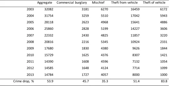
The context of decreasing property crime in Vancouver is shown in Table 1 and Fig .
2. Table 1 shows the counts of the four different crime types (commercial burglary,
mischief, theft from vehicle, theft of vehicle) as well as their aggregate. In 2003, the
most common form of property crime is theft from vehicle, followed by mischief and
theft of vehicle (effectively the same levels) and commercial burglary. However, by
2013, theft of vehicle has become the lowest volume property crime under analysis.
Overall, the crime drop for the aggregate of these crime types is 53.9 percent, a large
magnitude decrease in crime over an 11-year period. The distribution of this crime
drop is not uniform across the four crime types though. As would be expected
because of volume, theft from vehicle is the most similar to the aggregate, with
commercial burglary also exhibiting a similar drop. Mischief, however, exhibits a
notable lower magnitude crime drop (35.3 percent) and theft of vehicle exhibits a
substantial drop over this time period (83.8 percent) this drop has been
confirmed through conversations with police and vehicle insurance agencies as well
as with checks using other statistical sources.
This drop is further represented in Fig. 2 that shows the crime rates for the
City of Vancouver, calculated using the census population and linear interpolation
crime rates for 2003 were normalized to an index value of 100. Because of the small
magnitude population change relative to the changes in the crime counts
(population increased just below 10 percent, 2003 2013), there are no major
differences between Table 1 and Fig. 2, but the magnitude of the drop in theft of
vehicle is immediately apparent. This result is interesting in and of itself, but is
beyond the scope of the current analysis.
<Insert Fig. 2 and Table 1 About Here>
Turning to crime concentrations, Table 2 shows the percentage of street
segments and intersections that have any events for the four property crime types.
In the aggregate, only 35 percent of Vancouver had criminal events in 2003 and this
fell to just over 25 percent by 2013. This shows that in 2013, essentially 75 percent
of Vancouver was free from reported criminal activity for these crime types. Already
this is a high degree of concentration. When considering individual crime types, this
concentration becomes more apparent. Commercial burglary has remained
relatively stable in the percentage of locations it occurs, 4.5 to 7 percent. However, it
should be noted that commercial burglary can only occur where there is commercial
land use. As such, the high degree of concentration for this crime type is at least
partially artificial and a product of the urban landscape (owever the spatial
concentration of commercial burglary will be clearly evident in subseq uent tables.
Mischief has exhibited an increase in it spatial concentration over the study
period of approximately 30 percent. Theft from vehicle and theft of vehicle both
show increases in the spatial concentration of their criminal events, but the drop
knowledge that there has been a substantial drop in the volume of theft of vehicle,
this is an indication that theft of vehicle is no longer occurring in particular
locations. Again, though beyond the scope of the current analysis, this is an
intriguing spatial change.
<Insert Table 2 About Here>
Keeping in mind that all of the criminal events associated with these four
crime types can be considered spatially concentrated based on the percentages in
Table 2, Table 3 shows the percentage of street segments and street intersections
that account for 50 percent of criminal events in Vancouver. In the aggregate, these
numbers have not changed over time that is worthy of any discussion. However,
with only 3 to 4.5 percent of street segments and intersections required to account
for 50 percent of these criminal events, this is a high degree of spatial concentration
that is in line with previous research (Sherman et al., 1989; Weisburd, 2015).
Commercial burglary only requires just over 1 percent of locations to account for 50
percent of its criminal events and this percentage is stable over time. Theft from
vehicle is also generally stable over time, with some variability, at approximately 3
percent. However, mischief and theft of vehicle are exhibiting decreases in the
percentage of locations required to account for 50 percent of their criminal events:
3.5 to 2.5 percent and 5 to 2 percent, respectively. As such, not only are these crime
types spatially concentrated, but there is a concentration within that general
concentration; moreover, this latter concentration is becoming more pronounced
over time.
In the final investigation of crime concentrations, Table 4 shows the
percentage of street segments and street intersections with any crime that are
required to account for 50 percent of criminal events. Such a statistic identifies
concentrations within concentrations as well and accounts for land use issues for
commercial burglary. Overall, for the aggregate, 11 to 14 percent of locations that
have any crime are required to account for 50 percent of criminal events. This is a
high degree of spatial concentration within an already small percentage of places
that have any crime. There is a moderate decrease in this measure of spatial
concentration, indicating that criminal events are becoming relatively more uniform
over time, but this is not surprising given that the percentage locations with any
crime has been decreasing. Commercial burglary and theft from vehicle show
similar moderate increases in the percentage of locations with any crime required to
account for 50 percent of criminal events. Mischief, contrary to the other crime
types, though with some variability, has remained relatively constant at
approximately 20 percent.
The largest magnitude change is with regard to theft of vehicle. The
percentage of locations with any crime required to account for 50 percent of
criminal events has increased from 24 to 40 percent. As such, though the percentage
of locations with any theft of vehicle has decreased substantially, the spatial
distribution within that spatial concentration has become very close to uniform.
With fewer places theft of vehicle is occurring, however, such as result is not
unexpected but interesting nonetheless.
4.2. Pairwise spatial point pattern results
The results of the pairwise spatial point pattern tests for spatial stability are shown
in Tables 5 to 8. In each table, the upper-right triangle represents the spatial point
pattern test results using all street segments and street intersectio ns, whereas the
lower-left triangle represents the spatial point pattern test results only using street
segments and street intersections that have at least one criminal event in any given
year. This is a sensitivity analysis that we perform because all of the zero-values
may artificially inflate the S-Index values, indicating spatial stability when it is not
present within the places that experience crime. This set of street segments and
street intersections is different for each crime type under analysis , but the same for
all pairwise comparisons in order to be consistent with the longitudinal analyses .
The results for commercial burglary are shown in Table 5. Though we do not
want to consider the threshold value for the S-Index of 0.80 in a dichotomous
fashion, the upper-right triangle of Table 5 clearly shows a high degree of spatial
stability from year-to-year as well as over the entire study period; S-Index values
are all greater than 0.935. This bodes well for the spatial analysis of any given year
of data and making inferential statements regarding theoretical processes and the
development of criminal justice policy, specifically crime prevention initiatives. The
results for sensitivity analysis, only considering non-zero street segments and street
intersections, is not as favorable for spatial stability, particularly for the early years
in our study period. When comparing over time and year-to-year, there are very few
S-Index values greater than 0.70, 2003 2006. Only in the more recent years of the
stability. Therefore, when considering the entire city there appears to be a high
degree of spatial stability for commercial burglary, but when considering only those
locations where crime occurs, spatial stability only emerges in more recent years.
This indicates that there has been some degree of spatial change in the years of the
crime drop for commercial burglary in Vancouver.
The results for mischief, Table 6, are very similar to those for commercial
burglary. The S-Index values in the upper-right triangle of the table are always
greater than 0.84, indicating spatial stability when considering the entire city. The
sensitivity analysis does show an increasing degree of spatial stability in more
recent years, but the S-Index values are greater than those for commercial burglary
and approach the threshold value of 0.80 sooner, beginning in 2005.
Table 7 shows the results of the spatial point pattern test for theft from
vehicle. The S-Index values in the upper-right triangle for the entire city are now
mostly below the threshold value of 0.80, but still quite close so it would be difficult
to argue that there is not a high degree of spatial stability from 2003 to 2013 in
Vancouver. However, more similar to commercial burglary, the results of the
sensitivity analysis for theft from vehicle indicate that there is not spatial stability in
the set of locations that actually have criminal events of this type. With S-Index
values most often below 0.70 the case for spatial stability is difficult to make, even in
the more recent years under analysis.
And finally, Table 8 shows the S-Index values of the spatial point patterns test
for theft of vehicle. As with the previous results, those for theft of vehicle are
are always greater than 0.83, indicating a high degree of spatial stability in theft of
vehicle. Additionally, in the more recent years, 2010 to 2013, the S-Index values are
all greater than 0.90, similar to the results for commercial burglary. As such, there is
strong evidence for the presence of spatial stability at the level of the city even with
the large magnitude crime drop, 2003 2013. When only considering the street
segments and street intersections with any crime in the sensitivity analysis, the
early years in the study period do not exhibit a high degree of spatial stability, but in
more recent years, 2005 to 2013, there is strong evidence for spatial stability with
increasing values of the S-Index. This is particularly true for 2008 to 2013. This
evidence for spatial stability in theft of vehicle is particularly interesting given the
large magnitude crime that has occurred for this crime type in Vancouver over the
study period.
<Insert Tables 5 8 About Here>
4.3. Longitudinal spatial trajectories, 2003 2013
The overall pattern for the four crime types under investigation is relatively
consistent. When considering all street segments and intersections the S-Indices are
generally all above 0.80 theft from vehicle is the exception but those values are all
very close to 0.80 and when considering non-zero street segments and street
intersections, earlier S-Indices were moderately high (0.60 to 0.70) and approaching
the threshold of similarity in the later pairwise comparisons. This latter increase in
intersections in the data that have at least one criminal event in conjunction with
the crime drop the situation represented in Fig. 1b.
Despite the appearance of spatial stability, such pairwise comparisons,
though instructive, may not provide an accurate representation of spatial stability
over longer periods of time. In order to account for this possibility, the spatial point
pattern test was also conducted in a longitudinal manner to investigate the spatial
trajectories to account for the stability of crime patterns. These results are all shown
in Table 9.
<Insert Table 9 About Here>
Considering all street segments and intersections to be most consistent with
the more traditional trajectory analyses in the crime and place literature,
commercial burglary shows a remarkable degree of spatial stability over the 11
-year study period this is not an unexpected result given that commercial land use
is present in a small proportion of the city. Similarly, mischief, theft from vehicle,
and theft of vehicle all surpass the threshold of 0.80 for the SZero and SSum Indices. It
should be noted, however, that these two indices do not measure spatial stability in
its purest sense. SZero includes places that have seen potentially dramatic crime
decreases but have found a new stability and SSum includes places that may be
sporadic but will only impact the degree of similarity when a spatial unit of analysis
is generally stable with a few aberrations. As such, it is very important to a lso use
the index that measure pure, or absolute, stability, the SAbsolute Index. Though the
SAbsolute Index values are all below the 0.80 threshold for all crime types aside from
approaching the threshold and theft from vehicle has a moderately high index value.
Overall, particularly if one considers the crime drop leading to zero crime in some
places, the spatial trajectories of these crime types in Vancouver are remarkably
stable over time.
Considering the non-zero street segments and intersections, stability is not
as high, showing the importance of removing the zero -values when considering the
stability of crime patterns in a supplementary analysis. Street segments and
intersections that do not have any crime over the study period is a form of stability.
Consequently, this is an important result that needs to be identified. However, if the
researcher is interested in knowing how stable spatial crime patterns are in those
places in which crime actually occurs, a supplementary analysis that only considers
non-zero spatial units of analysis becomes important. Considering non -zero street
segments and intersections, all crime types have SAbsolute Index values less than 0.51
indicating a low level of stability over the study period. However, the SZero and SSum
Indices are approaching the 0.80 threshold (and achieving that threshold for theft of
vehicle), indicating a moderate degree of stability in crime patterns pa rticularly if
one considers the crime drop represented in Fig. 1b.
These results show that the pairwise comparisons discussed above are
generally consistent with the longitudinal spatial trajectories. However, caution
must be undertaken when making longer-term inferences from pairwise
5. DISCUSSION
In this paper, we have investigated crime concentrations and the spatial stability of
crime patterns for four property crime types in Vancouver, British Columbia, 2003
2013. With regard to crime concentrations, we find that crime is highly
concentrated in few locations in Vancouver. And, in most case s, these crime
concentrations have been increasing while crime volumes have been decreasing.
This is a particularly interesting phenomenon that needs further investigation. In
the case of Vancouver, two things are occurring. First, crime is going down almost
everywhere. This overall decrease was present in previous research on Vancouver
(Curman et al., 2015) and in the current data. Also, the crime types investigated in
this paper have disappeared from particular street segments and street
intersections. Overall for the city, 65 percent of Vancouver was free from these
(police-reported) crime types in 2003 compared to 75 percent of Vancouver in
2013. With lower volumes of crime, fewer micro-places are necessary to account for
50 percent of the criminal events, as evidenced in Tables 2 and 3.
Perhaps more interesting is the consideration of Table 4. When considering
all of the street segments and intersections, crime is dropping and becoming more
concentrated. However, when one considers only the places in which crime is
occurring, crime is becoming more dispersed mischief is the exception. So, there is
less crime, it is occurring in fewer places, but within those fewer places the
distribution of criminal events is becoming more evenly distributed, particularly for
theft of vehicle. Why? Consider the case of theft of vehicle. This crime type exhibited
percentage of street segments and intersections (micro-places) with any theft of
vehicle dropped by approximately 75 percent. At the same time, the percentage of
micro-places that account for 50 percent of criminal events decreased by a little
more than one-half. Given that the percentage of micro-places with any theft of
vehicle decreased by a greater degree than the percentage of micro-places that
account for 50 percent of theft of vehicle, the percentage of micro-places with any
thefts of vehicle that account for 50 percent of thefts of vehicle must necessarily
increase. There were simply fewer places for those criminal events to occur.
Consequently, those researching crime at places and spatial concentrations
must be cautious to not take these statistics at face value. They are important and
tell a story of changes in spatial patterns of crime, but they should not impre ss us at
face value. This is similar to a crime type that is relatively rare, say 1000 events over
the course of a year, that is counted in the context of micro -places. If there are
10,000 micro-places and one criminal event per micro-place, the minimum level of
concentration over the entire city is 10 percent: 1000/10,000. Stating that 90
percent of the city is free from this crime type seems to be an impressive
concentration but such a concentration is actually uniform it isn t a
concentration at all. This is precisely the case for theft of vehicle in Vancouver
during 2013: 1000 criminal events, approximately 20,000 micro -places and
approximately 5 percent of the entire city that experiences this crime type. In fact,
the most dispersed this crime type can be is being present in 5.4 percent of
micro-places. Consequently, theft of vehicle is hardly concentrated at all when one
percent of micro-places to account for 50 percent of criminal events makes perfect
sense. Yes, this crime type is incredibly concentrated within the entire city, but we
must consider the nature and possibilities of that concentration given our chosen
spatial units of analysis.
The flipside of these concentrations is the degree of change in the spatial
patterns of crime. With 35 percent of micro-places having one of these four crime
types in 2003 and only 25 percent in 2013, there is a lot of crime concentration at
both points in time. However, there has also been substantial change. As shown
using the longitudinal version of the spatial point pattern test (Table 9), a lot of the
change can be explained considering those micro -places that cease to have criminal
events (Fig. 1b): the SAbsolute Index versus the SZero Index. But where is the rest of the
change occurring? Part of this change is occurring through the simple mathematics
of places described above: crime concentrations change because there is nowhere
else for the criminal events to go that will not impact the spatial stability of crime
and, hence, the spatial trajectories. This does not mean that we do not need to
investigate any socio-demographic or socio-economic changes that have led to
subsequent changes in crime patterns, but we must recognize that a lot of the
changes shown above can be understood based on simple explanations: crime just
stopped occurring in particular places and became more evenly dispersed as a
result. However, socio-demographics and/or socio-economics may come into play to
understand why particular micro-places no longer had crime, but this is beyond the
Returning to the question of whether the law of crime concentration at
places is simply a manifestation of the concentration of human activities more
generally, we begin to shed light on this question through a comparison of the
results for commercial burglary and vehicle-related crime. Vehicle-related crime can
occur wherever there is the presence of vehicles, whereas commercial burglary can
only occur where there is commercial or mixed land use, by definition.
Consequently, if the law of crime concentration at places is simply a specific
manifestation of the concentration of human activities, more generally, commercial
burglary will always be more concentrated than vehicle-related crime. General
support for this proposition is found in Tables 2 and 3, given that commercial
burglary is always more concentrated than theft from vehicle and more
concentrated than theft of vehicle in all but one case. However, because the degrees
of concentration for commercial burglary and theft of vehicle are converging over
time, this shows that the concentration of human activities is not enough to explain
the law of crime concentration at places. This will prove to be an interesting avenue
of future research, considering specific crime types and the availability of
opportunities based on the general concentrations of human activities.
Overall, when considering spatial stability for the entire city, we find strong
evidence for the presence of spatial stability. This bodes well for theoretical testing
and development as well as the development of criminal justice policy, specifically
crime prevention initiatives. When only considering street segments and street
intersections that have any crime, the results for spatial stability are less promising
stability in the sensitivity analyses, but generally speaking spatial stability in the
locations that actually have crime has a shorter time horizon.
The implications for theory from these results are that there is a relatively
high degree of spatial stability at the level of the city. As such, if the testing of theory
and any subsequent refinements are based on city-level analyses, using street
segments or census tracts as the units of analysis, for example, there are probably
not going to be any difficulties. However, if local area analyses are being undertaken
to investigate the nuances of theoretical predictions, then caution should be
undertaken for generalizing if a longer period of time has elapsed. This is especially
the case when the volume of crime is changing.
In the context of criminal justice policy, specifically crime prevention
initiatives, the same general statements can be made. However, specifically in the
case of situational crime prevention that is quite spatially-specific, the importance of
having recent crime data is paramount. Even with S-Index values greater than 0.80
there is still a great degree of spatial change occurring: 20 percent of 18,455 spatial
units of analysis is still 3689 street segments and street intersections that are
exhibiting change. An argument for spatial stability can be made for the overall
crime pattern, but this may not be spatially stable enough for situational crime
prevention.
Though instructive, our analyses are not without their limitations. First and
foremost, we are restricted to police-reported crime data and a small number of
crime types. There is little we can do regarding this limitation, however. Relatedly,
reporting, citizen reporting, and police patrol activities; however, mischief does not
present any results that are qualitatively different from the other crime types.
Second, our data do not have specific addresses or geographic coordinates available,
but we do restrict all inference to the street segment or street intersection in order
to avoid the ecological fallacy. And third, our time frame is only 11 years. Though
there are not many longitudinal criminal event data sets available there is little that
can be done regarding this limitation aside from waiting for more years to pass,
assuming more years of data will continue to be available for these cities. However,
with evidence of spatial stability in the 10 years prior to this study (Curman et al.,
2015), we should be able to move forward with cautious optimism with regard to
spatial stability.
As with most research, our analyses raise more questions than answer ed and
these guide future directions for research. First and foremost is the importance of
further replication. In order to move forward with (social) science, our results must
be replicated in other contexts: are spatial trajectories stable over time in other
cities? Second, traditional trajectory analyses of these data would prove to be
instructive. A comparison of the results presented here considering the spatial
trajectory should be compared with the various classifications that would emerge
from a traditional trajectory analysis. Are the various clusters of traditional
trajectories when compared with the locations that exhibit spatial stability or not in
the same places? It would be interesting to know if traditional trajectories classified
as stable would include the street segments and street intersections that are
spatial point pattern test, and vice versa. And finally, further investigations into the
changing patterns of theft of vehicle are in order. With such a large magnitude crime
drop and increasingly concentrated crime types, there are most certainly interesting
REFERENCES
Andresen, M. A. (2009). Testing for similarity in area-based spatial patterns: A
nonparametric Monte Carlo approach. Applied Geography 29: 333 345.
Andresen, M. A. (2010). Canada - United States interregional trade: quasi-points and
spatial change. Canadian Geographer 54: 139 - 157.
Andresen, M. A., and Linning, S. J. (2012). The (in)appropriateness of aggregating
across crime types. Applied Geography 35: 275 - 282.
Andresen, M. A., and Malleson, N. (2011). Testing the stability of crime patterns:
Implications for theory and policy. Journal of Research in Crime and
Delinquency 48: 58 - 82.
Andresen, M. A., and Malleson, N. (2013a). Spatial heterogeneity in crime analysis. In
M. Leitner (ed.), Crime Modeling and Mapping Using Geospatial Technologies,
Springer, New York, pp. 3 - 23.
Andresen, M. A., and Malleson, N. (2013b). Crime seasonality and its variations
across space. Applied Geography 43: 25-35.
Andresen, M. A., and Malleson, N. (2014). Police foot patrol and crime displacement:
A local analysis. Journal of Contemporary Criminal Justice 30: 186-199.
Boyce, J., Cotter, A., and Perreault, S. (2014). Police-Reported Crime Statistics in
Canada, 2013, Statistics Canada, Canadian Centre for Justice Statistics,
Ottawa, ON.
Braga, A., Hureau, D. M., and Papachristos, A. V. (2011). The relevance of micro
places to citywide robbery trends: A longitudinal analysis of robbery
Crime and Delinquency 48: 7 32.
Bursik, R. J. Jr. (1988). Social disorganization and theories of crime and delinquency:
Problems and prospects. Criminology 26: 519 551.
Curman, A. S. N., Andresen, M. A., and Brantingham, P. J. (2015). Crime and place: a
longitudinal examination of street segment patterns in Vancouver, BC.
Journal of Quantitative Criminology 31: 127 - 147.
Davis, T. J., and Keller, C. P. (1997). Modelling uncertainty in natural resource
analysis using fuzzy sets and Monte Carlo simulation: Slope stability
prediction. International Journal of Geographical Information Science 11:
409 434.
Farrell, G., Tseloni, A., Mailley, J., and Tilley, N. (2011). The crime drop and the
security hypothesis. Journal of Research in Crime and Delinquency 48: 147
175.
Farrell, G., Tilley, N., and Tseloni, A. (2015). Why the crime drop? Crime and Justice
43: 421 490.
Groff, E. R., Weisburd, D., and Yang, S-M. (2010). Is it important to examine crime
trends at a local micro level A longitudinal analysis of street to street
variability in crime trajectories. Journal of Quantitative Criminology 26: 7
32.
Hope, A. C. A. (1968). A simplified Monte Carlo significance test procedure. Journal
of the Royal Statistical Society, Series B 30: 583 598.
Kong, R. (1997). Canadian Crime Statistics, 1996, Statistics Canada, Canadian Centre
Lees, L., Slater, T., and Wyly, E. K. (2007). Gentrification, Routledge, New York.
Linning, S .J. (2015). Crime seasonality and the micro-spatial patterns of property
crime in Vancouver, BC and Ottawa, ON. Journal of Criminal Justice 43: 544
555.
O Brien R M A caution regarding rules of thumb for variance inflation
factors. Quality & Quantity 41: 673 690.
Ratcliffe, J. H. (2004). Geocoding crime and a first estimate of a minimum acceptable
hit rate. International Journal of Geographical Information Science 18: 61
72.
Savoie, J. (2002). Crime Statistics in Canada, 2001, Statistics Canada, Canadian Centre
for Justice Statistics, Ottawa. ON.
Shaw, C. R., Zorbaugh, F., McKay, H. D., and Cottrell, L. S. (1929). Delinquency areas:
A study of the geographic distribution of school truants, juvenile delinquents,
and adult offenders in Chicago, University of Chicago Press, Chicago.
Shaw, C. R. and McKay, H. D. (1931). Social factors in juvenile delinquency, U.S.
Government Printing Office, Washington, DC.
Shaw, C. R. and McKay, H. D. (1942). Juvenile delinquency and urban areas: A study of
rates of delinquency in relation to differential characteristics of local
communities in American cities, University of Chicago Press, Chicago.
Shaw, C. R. and McKay, H. D. (1969). Juvenile delinquency and urban areas: A study of
rates of delinquency in relation to differential characteristics of local
communities in American cities (revised edition), University of Chicago Press,
Sherman, L. W., Gartin, P. R., and Buerger, M. E. (1989). Hot spots of predatory
crime: routine activities and the criminology of place. Criminology 27: 27 55.
Silver, W. (2007). Crime Statistics in Canada, 2006, Statistics Canada, Canadian
Centre for Justice Statistics, Ottawa, ON.
Tompson, L., Johnson, S., Ashby, M., Perkins, C., and Edwards, P. (2015). UK open
source crime data: accuracy and possibilities for research. Cartography and
Geographic Information Science 42: 97 111.
Tseloni, A., Mailley, J., Farrell, G., and Tilley, N. (2010). Exploring the international
decline in crime rates. European Journal of Criminology 7: 375 394.
Wallace, M. (2003). Crime Statistics in Canada, 2002, Statistics Canada, Canadian
Centre for Justice Statistics, Ottawa, ON.
Wallace, M. (2004). Crime Statistics in Canada, 2003, Statistics Canada, Canadian
Centre for Justice Statistics, Ottawa, ON.
Weisburd, D. (2015). The law of crime concentration and the criminology of place.
Criminology 53: 133 157.
Weisburd, D., and Amram, S. (2014). The law of concentrations of crime at place:
The case of Tel Aviv-Jaffa. Police Practice and Research 15: 101 114.
Weisburd, D., Bushway, S., Lum, C. and Yang, S-M. (2004). Trajectories of crime at
places: A longitudinal study of street segments in the City of Seattle.
Criminology 42: 283 321.
Weisburd, D., Groff, E. R., and Yang, S-M. (2012). The criminology of place: Street
segments and our understanding of the crime problem, Oxford University
Weisburd, D., Morris, N. A. and Groff, E. R. (2009). Hot spots of juvenile crime: A
longitudinal study of street segments in Seattle, Washington. Journal of
Table 1. Count of crime types, Vancouver, 2003 2013
Aggregate Commercial burglary Mischief Theft from vehicle Theft of vehicle
2003 32082 3181 6270 16459 6172
2004 31754 3259 5510 17042 5943
2005 28118 2623 4968 15641 4886
2006 25860 2828 5199 14227 3606
2007 22332 2430 4825 11857 3220
2008 20816 2216 5345 10924 2331
2009 17680 1830 4380 9626 1844
2010 15729 1625 4376 8307 1421
2011 14390 1608 4596 7132 1054
2012 14585 1648 4124 7714 1099
2013 14784 1727 4057 8000 1000
Table 2. Percent of street segments and street intersections with any crime
Aggregate Commercial burglary Mischief Theft from vehicle Theft of vehicle
2003 34.77 6.41 16.62 24.87 17.86
2004 36.58 6.81 15.89 27.05 18.77
2005 35.41 6.40 14.69 26.22 16.99
2006 32.32 6.45 15.01 23.25 13.07
2007 30.14 5.80 13.44 20.71 12.13
2008 28.24 5.59 14.53 18.64 9.28
2009 27.86 5.03 13.41 18.86 8.18
2010 27.57 4.49 12.71 19.50 6.45
2011 26.39 4.49 12.93 18.09 4.98
2012 26.50 4.90 12.29 19.01 5.13
Table 3. Percent of street segments and street intersections that account for 50% of crime
Aggregate Commercial burglary Mischief Theft from vehicle Theft of vehicle
2003 3.75 1.20 3.34 2.50 4.27
2004 4.34 1.23 3.49 3.10 4.96
2005 4.46 1.31 3.37 3.17 4.77
2006 3.68 1.26 3.22 2.50 3.59
2007 3.21 1.13 2.75 2.10 3.40
2008 2.86 1.19 2.80 1.65 2.69
2009 3.37 1.08 3.12 2.24 3.18
2010 3.85 1.01 2.68 3.12 2.60
2011 3.75 0.92 2.46 3.21 2.12
2012 3.84 1.16 2.61 3.18 2.15
Table 4. Percent of street segments and street intersections with any crime that account for 50% of crime
Aggregate Commercial burglary Mischief Theft from vehicle Theft of vehicle
2003 10.79 18.68 20.10 10.05 23.92
2004 11.87 18.06 21.94 11.47 26.42
2005 12.59 20.41 22.96 12.10 28.05
2006 11.37 19.60 21.46 10.77 27.47
2007 10.67 19.55 20.49 10.13 28.03
2008 10.14 21.24 19.25 8.87 28.99
2009 12.11 21.47 23.29 11.87 38.90
2010 13.96 22.44 21.11 16.01 40.34
2011 14.20 20.39 18.99 17.74 42.59
2012 14.48 23.70 21.22 16.74 41.97
Table 5. Indices of similarity, 2003-2013, Vancouver, commercial burglary, street segments & intersections and non-zero street segments & intersections
2003 2004 2005 2006 2007 2008 2009 2010 2011 2012 2013
2003 0.940 0.941 0.939 0.941 0.938 0.940 0.940 0.939 0.940 0.939
2004 0.678 0.937 0.939 0.938 0.942 0.939 0.947 0.936 0.943 0.936
2005 0.681 0.659 0.940 0.941 0.942 0.940 0.949 0.941 0.944 0.940
2006 0.668 0.672 0.679 0.941 0.941 0.940 0.948 0.941 0.944 0.938
2007 0.682 0.664 0.682 0.680 0.949 0.946 0.951 0.945 0.946 0.945
2008 0.681 0.691 0.690 0.686 0.727 0.949 0.952 0.949 0.947 0.949
2009 0.680 0.770 0.681 0.675 0.713 0.732 0.957 0.952 0.951 0.951
2010 0.683 0.719 0.727 0.723 0.735 0.740 0.770 0.957 0.950 0.957
2011 0.672 0.662 0.681 0.685 0.708 0.727 0.744 0.764 0.953 0.957
2012 0.675 0.694 0.702 0.697 0.706 0.725 0.739 0.729 0.750 0.954
2013 0.675 0.655 0.674 0.670 0.703 0.720 0.734 0.767 0.765 0.754