INFORMS is located in Maryland, USA
Transportation Science
Publication details, including instructions for authors and subscription information: http://pubsonline.informs.org
Travel-Time Models With and Without Homogeneity Over
Time
Malachy Carey, Paul Humphreys, Marie McHugh, Ronan McIvor
To cite this article:
Malachy Carey, Paul Humphreys, Marie McHugh, Ronan McIvor (2017) Travel-Time Models With and Without Homogeneity Over Time. Transportation Science 51(3):882-892. https://doi.org/10.1287/trsc.2016.0674
Full terms and conditions of use: http://pubsonline.informs.org/page/terms-and-conditions
This article may be used only for the purposes of research, teaching, and/or private study. Commercial use or systematic downloading (by robots or other automatic processes) is prohibited without explicit Publisher approval, unless otherwise noted. For more information, contact [email protected].
The Publisher does not warrant or guarantee the article’s accuracy, completeness, merchantability, fitness for a particular purpose, or non-infringement. Descriptions of, or references to, products or publications, or inclusion of an advertisement in this article, neither constitutes nor implies a guarantee, endorsement, or support of claims made of that product, publication, or service.
Copyright © 2016, The Author(s)
Please scroll down for article—it is on subsequent pages
INFORMS is the largest professional society in the world for professionals in the fields of operations research, management science, and analytics.
Vol. 51, No. 3, August 2017, pp. 882–892 http://pubsonline.informs.org/journal/trsc/ ISSN 0041-1655 (print), ISSN 1526-5447 (online)
Travel-Time Models With and Without Homogeneity Over Time
Malachy Carey,a, bPaul Humphreys,aMarie McHugh,aRonan McIvora
aUlster University Business School, Ulster University, Belfast BT37 0QB, United Kingdom; bInstitute for Transport Studies,
University of Leeds, Leeds LS2 9JT, United Kingdom
Contact: [email protected](MC); [email protected](PH); [email protected](MM); [email protected](RM)
Received:March 19, 2014
Revised:November 11, 2014; September 1, 2015
Accepted:November 28, 2015
Published Online in Articles in Advance:
May 31, 2016
https://doi.org/10.1287/trsc.2016.0674
Copyright:© 2016 The Author(s)
Abstract. In dynamic network loading and dynamic traffic assignment for networks, the link travel time is often taken as a function of the number of vehiclesx(t)on the link at timetof entry to the link, that is,τ(t)f(x(t)), which implies that the performance of the link is invariant (homogeneous) over time. Here we let this relationship vary over time, letting the travel time depend directly on the time of day, thusτ(t)f(x(t),t). Various authors have investigated the properties of the previous (homogeneous) model, including conditions sufficient to ensure that it satisfies first-in-first-out (FIFO). Here we extend these results to the inhomogeneous model, and find that the new sufficient conditions have a natural interpretation. We find that the results derived by several previous authors continue to hold if we introduce one additional condition, namely that the rate of change of f(x(t),t)with respect to the second parameter has a certain (negative) lower bound. As a prelude, we discuss the equivalence of equations for flow propagation equations and for intertemporal conservation of flows, and argue that neither these equations nor the travel-time model are physically meaningful if FIFO is not satisfied. In Section7we provide some examples of time-dependent travel times and some numerical illustrations of when these will or will not adhere to FIFO.
Open Access Statement:This work is licensed under a Creative Commons Attribution 4.0 International License. You are free to copy, distribute, transmit and adapt this work, but you must attribute this work as “Transportation Science.©2016 The Author(s).https://doi.org/10.1287/trsc.2016.0674, used under a Creative Commons Attribution License:http://creativecommons.org/licenses/by/4.0/.” Funding:The authors wish to thank the UK Engineering and Physical Science Research Council
(EPSRC) for supporting this research [Grant EP/G051879].
Keywords: travel-time functions • first-in-first-out • homogeneity • dynamic network loading • dynamic traffic assignment
1. Introduction
The travel time for each link in a network, in dynamic network loading (DNL) and dynamic traffic assign-ment (DTA), has often been modeled as a function of the number of vehicles x(t)on the link, thus f(x(t)),
so that for a user entering a link at timetthe link exit time is
τ(t)t+f(x(t)). (1)
The variablex(t) is also referred to as the link
occu-pancy and is given by the conservation equation
x(t)
∫ t
0
u(s)ds−
∫ t
0
v(s)ds, (2)
whereu(t)andv(t)are the inflow and outflow,
respec-tively, at timet.
This model and its use in DNL and DTA has been investigated in many papers and is included in reviews such as Peeta and Ziliaskopoulos (2001), Szeto and Lo (2005,2006), Friesz, Kwon, and Bernstein (2007), and Mun (2007,2009). Some properties of the model when used in DNL or DTA are discussed and illustrated in
Friesz et al. (1993), Xu et al. (1999), Zhu and Marcotte (2000), Carey and Ge (2005b), Carey (2004), Carey and McCartney (2002), Nie and Zhang (2005a), and Zhang and Nie (2005): the first four of these papers are dis-cussed at greater length in this paper. The behavior and performance of the model is compared with other macroscopic whole-link models used in DTA in Carey
and Ge (2003a), and Nie and Zhang (2005b).
Com-putational issues for applying the model in DTA are discussed in Rubio-Ardanaz, Wu, and Florian (2003), Carey and Ge (2004,2005a), Nie and Zhang (2005a,b), and Long, Gao, and Szeto (2011).
In the previous model it is assumed that, given the current occupancy x(t) of a link, the link travel time
is independent of time. However, in practice the link travel time predicted at the time of entry to a link may also vary over time during the day as a result of fac-tors other than the number of vehicles on the link. These factors include time-varying traffic control sig-nals, signs, speed limits, changing visibility because of the transition from day to night and vice versa,
882
time-varying traffic mix, or changing weather condi-tions, such as the onset of rain, fog, snow, etc. (see Sec-tion7). Note that changing weather conditions (rain, fog, snow, etc.) are usually of a stochastic nature, for which the deterministic models in this paper are not a suitable framework for prediction purposes. It is easy to formally extend the previous model to allow the link travel time to depend on the time of day as well as the current occupancy of the link, thus f(x(t),t), so that
the link exit time is
τ(t)t+f(x(t),t). (3)
There is a long history of papers proposing and dis-cussing various functional forms for the travel time functions f(x(t))in (1), including Branston (1976), Ran
and Boyce (1996), Ran et al. (1997), and Anderson and Bell (1998), so we do not repeat the discussion of func-tional forms here. Also, over the past 15 years many methods have been proposed and used to estimate these travel-time functions for links or routes. Many authors suggest using transit vehicles or taxi fleets as probes with sensors, or using automatic vehicle loca-tion (AVL), typically using GPS. Others recommend using automatic vehicle or number plate identification, using cell phone data, or using loop detectors. One thing that all of these methods have in common is that the time of day is automatically or easily available in the data collection process and hence in the resulting data sets. This facilitates treating the time of day as a factor in estimating and predicting travel times and thus in estimating functions of the form f(x(t),t)used
in (3). For example, Zhang, Wu, and Kwon (1997) note that regression based methods can easily incorporate various factors that affect travel time, one of the fac-tors being time of day. Again, we do not repeat the discussion of functional forms or estimation methods for f(x(t),t), other than in the first few paragraphs of
Section7.
The properties of the model (1)–(2) have been de-rived in several papers but it is not known, and is not immediately obvious, how the properties of this model are affected by extending it to allow inhomogeneity over time, as in (2)–(3). We therefore investigate this in the present paper. In particular, we investigate the conditions needed to ensure that the model still retains desirable first-in-first-out (FIFO) properties. The main mathematical properties of the model (1)–(2), includ-ing FIFO, were rigorously derived in Friesz et al. (1993), Xu et al. (1999), and Zhu and Marcotte (2000). Carey and Ge (2005b) took some of the conditions or restric-tions derived in Xu et al. (1999) and Zhu and Marcotte (2000), and replaced them with conditions or restric-tions that may be more easily checked or more likely to be satisfied. In this paper we take the properties derived in these four papers for model (1)–(2) and seek to extend them to the model (2)–(3).
In Section 2 we complete the models (1)–(2) and (2)–(3) by setting out flow propagation equations, which we note can be interpreted as intertemporal link conservation equations, and discuss the relationship between these and FIFO. In Sections3–6, respectively, we take the properties of the model (1)–(2), derived in the four papers previously noted, and investigate whether and how these extend to the model (2)–(3). Section4 assumes a linear form of f(x(t),t) and
Sec-tions4–6assume a nonlinear form. In Section7we pro-vide some examples of time-dependent travel times and some numerical illustrations of when these will or will not satisfy FIFO. Concluding remarks are in Section8.
2. Letting Travel-Time Vary with Time:
Inhomogeneous Travel-Time Functions
In the real world of road traffic, FIFO is not strictly adhered to, since many vehicles overtake and pass each other. Such overtaking or passing could potentially be modeled, but it is not explicitly modeled or included in the travel-time models (1)–(2) or (2)–(3). Nevertheless, if certain technical properties are not satisfied, these models can allow traffic cohorts to overtake or pass each other and in ways that can differ substantially from what happens in the real world and may not even be physically possible in the real world. For example, if certain technical properties are not satisfied, we find that if the inflow u(t) to a link is falling rapidly over
a short time interval then, based on (1)–(2), all of the traffic that enters the link in that time interval may exit before traffic that entered earlier when the inflow rate was higher, which violates FIFO. That does not reflect any real world behavior, which is why we wish to prevent such FIFO violations in the travel-time mod-els (1)–(2) and (2)–(3).
Completing the model: Intertemporal flow conserva-tion or flow propagaconserva-tion and FIFO. The link travel-time model is often stated as (1)–(2) together with a so-called flow propagation equation such as (4) or (5) in the next paragraph. We note that (2) is a contemporaneous con-servation equation and, as we will see shortly, if FIFO holds then the flow propagation equation can also be interpreted as an intertemporal conservation equation. Thus, the travel-time model consists of (1) subject to a contemporaneous conservation Equation (2) and an intertemporal conservation equation such as (4) or (5). FIFO is not imposed as a separate or additional con-straint, but must be inherent in (1) subject to these two forms of conservation equations. To show that FIFO holds for any particular form of f(x(t)) in (1)
requires a proof: e.g., proofs are given for a linear
f(x(t))in Friesz et al. (1993) and for the linear and
non-linear f(x(t))in Xu et al. (1999) and Zhu and Marcotte
(2000). These remarks refer to the homogeneous travel-time travel function (1), but we will see that they can
be extended to the inhomogeneous travel-time func-tion (3), so that the inhomogeneous travel-time model consists of (3) subject to the same contemporaneous conservation Equation (2) and the same intertemporal conservation equation such as (4) or (5).
The flow-propagation equation is written in various forms in the literature, in particular
∫ t
−∞
u(s)ds
∫ τ(t) −∞
v(s)ds, (4)
where u(s)and v(s)are the inflow and outflow from
the link at times, or alternatively
x(τ(t))
∫ τ(t) t
u(s)ds, (5)
wherex(τ(t))is the number of vehicles on the link at
timeτ(t). The flow-propagation equation is sometimes
stated withtdefined as the exit time andt−τ∗(
t)as the
entry time, whereτ∗(
t)is the link travel time for traffic
that exits at timet. Furthermore, the flow-propagation equation is sometimes stated as the derivative of any of these forms. All of these forms are derivable from each other hence we will not discuss them explicitly here.
If FIFO holds then it is easy to see that (4) and (5) are simply intertemporal conservation equations. More specifically, if FIFO holds for all traffic entering up to timeT, then we can see that (4) holding for all time 0≤ t≤Tis necessary and sufficient to ensure conservation
of flows up to timeT. Similarly for (5) if it holds for all time 0≤t≤T. For example, if FIFO holds then all traffic
that entered up to timetmust have exited by timeτ(t),
so that the only traffic still on the link at timeτ(t)must
have entered between timetandτ(t), i.e.,∫τ(t)
t u(s)ds,
and if flow is conserved this traffic is still on the link, so that (5) holds.
Now suppose that FIFO does not hold and consider Equations (4) or (5). If FIFO is violated then some inflowsu(s) that entered before timetmay not exit until after timeτ(t), and conversely some inflowsu(s)that
entered after timet may exit before timeτ(t). Neither
of these flows is captured by (4) or (5) hence if FIFO is violated then imposing (4) or (5) would seem to have no physical justification, and is likely to produce non-sense results. If FIFO does not hold then neither (4) nor (5) nor any of the other proposed forms of flow propagation equations will ensure intertemporal con-servation of flows. Also, if FIFO does not hold, it is not at all obvious that there is any form of equation that would ensure intertemporal flow conservation for the model (1)–(2) or (2)–(3).
In summary,
(a) If FIFO holds on a link, then an intertemporal flow conservation equation for the link is equivalent to
the flow propagation equation used elsewhere in the literature.
(b) If FIFO does not hold then neither the flow con-servation nor flow-propagation equations make physi-cal sense and it is not appropriate to impose them. In view of that, we will refer to intertemporal flow con-servation rather than flow propagation.
Before leaving the matter in (b), namely flow con-servation equations without FIFO, it is worth noting that even though this is not physically meaningful, a model that allows it may still have a mathematical solu-tion. For example, suppose that the only traffic on a link enters between times t1 and t2 and these inflows
all violate FIFO by exiting in the reverse of the order in which they entered and consequently τ(t
2)< τ(t1).
Applying (5) at time t1 and again at timet2>t1 and
subtracting the former from the latter gives an alterna-tive form of the conservation equation, namely
∫ t2
t1
u(s)ds
∫ τ(t2)
τ(t
1)
v(s)ds. (6)
As a result of the FIFO violation, on the right-hand side (r.h.s.) of (6) the upper limit of integration is smaller than the lower limit, hence the r.h.s. of (6) is negative, if we treat the outflows v(t)as positive. However, the
left-hand side (l.h.s.) is positive thus we seem to have a contradiction. There is no mathematical difficulty in solving (6) because (6) will simply yield negative out-flows v(t), not because they are physically negative
(they are not), but because the time span over which the outflowsv(t)occur is measured backwards in time.
In Sections 3–6, respectively, we take results from four different papers concerning the homogeneous
case (1) and extend them to the inhomogeneous
case (3). In all four cases we find that the results from the homogeneous case, including the results concern-ing FIFO, continue to hold for the inhomogeneous case if the following condition also holds:
ft(x,t)>−u(t)/B, (7)
whereBis an upper bound onu(t).
Some further implications and interpretations of (7) are discussed in Section7. We make just two remarks concerning it here before embarking on derivations of (7) in Sections3–6.
(i) If inflow u(t) is at its upper bound B then (7)
reduces to ft(x,t)>−1 and if inflow is at its lower
boundu(t)0 then (7) reduces to f
t(x,t)>0.
(ii) The FIFO sufficient condition (7) depends on the inflow profile u(t) and its upper bound B, which is
a disadvantage because the inflows are likely to vary over time and in a network model the inflows to each link are generally not known in advance. It would be nice to have a FIFO condition that is independent of
the inflows. However, it is well known that such a suf-ficient condition for FIFO is not available even for the homogeneous casef(x)when the travel time functions f(x) are nonlinear. In that (nonlinear) homogeneous
case the only available condition sufficient to ensure FIFO is as follows (see Xu et al.1999; Zhu and Marcotte
2000) or Section4and5
fx(x)<1/B, (8)
whereBis defined as in (7), i.e., it is the upper bound on the inflowsu(t).
Each of the four papers considered in Section 3–6
assume a travel-time function of the form f(x(t))used
in (1). For each of these papers we extend some key results, particularly concerning FIFO, to travel-time functions of the inhomogeneous form f(x(t),t) used
in (3). The theorems or propositions and their proofs in those four papers are quite lengthy so we do not wish to repeat them here. Instead we present only the changes that are needed to extend the theorems or propositions and proofs to the inhomogeneous case (3). Each of the papers discussed in the following sec-tions makes use of a well-known necessary and suf-ficient condition for FIFO for any form of travel-time model, namely that for traffic entering at timet, its exit timeτ(t)should be an increasing function oft. Thus,
assuming that τ(t) is differentiable, this FIFO
condi-tion is
τ0(
t)>0, (9)
where the prime(0)
denotes a first derivative.
3. Extending the Results from
Friesz et al. (1993) to the
Inhomogeneous Case
[The notation used in Friesz et al. (1993) is the same
as in this paper except that they use D to denote
link travel-time functions while we use f, as in (10) and (11).]
In Section3of their paper Friesz et al. (1993) intro-duce and derive properties of a linear travel-time func-tion or delay model
f(x(t))αx(t)+β, (10)
where x(t) is as previously defined and α ≥0 and β >0 are constants. To extend this to an inhomoge-neous function, while retaining linearity, add a term γ(t), thus
f(x(t),t)αx(t)+β+γ(t). (11)
Note thatβandγ(t)can of course be combined, letting γ∗(
t)β+γ(t). Friesz et al. (1993) derive properties of
the linear model (10) in their Theorem1as follows.
Theorem 1 of Friesz et al. (1993). For any linear arc delay function f, the resulting arc exit time function τ is strictly increasing and hence the inverse functionτ−1
exists.
Following the theorem Friesz et al. (1993) note that this (an increasing exit time function) implies that the model satisfies FIFO, as also noted in (9). We can extend their results to an inhomogeneous linear travel-time model (11) as follows.
Proposition 1. If the travel-time function (10) is replaced by (11) then Theorem1from Friesz et al. (1993) continues to hold if we also let
γ0(
t) ≥ −αu(t),or equivalentlyγ0(
t) ≥ −u(t)/B, (12)
whereγ0(
t)denotes the derivativedγ(t)/dtand1/αB.
Remark. The parameter αin (10) is often interpreted as 1/B where Bis the maximum flow capacity of the
link in the static or steady state case. To see this, note that in the steady state case we have an identityxus
where x is link occupancy, u is the flow rate, and s
is the link trip time. Using the linear travel-time func-tion sαx+β to substitute for s in xus gives a flow-occupancy function ux/(αx+β). The latter is
everywhere increasing and is asymptotic from below to 1/α. Therefore, the linear travel-time functions (10)
imply that the flow u is bounded above by 1/α.
Let-ting 1/αB we can rewriteγ0(
t) ≥ −αu(t)from (12)
asγ0(
t) ≥ −u(t)/B. The advantage of the latter form is
that it is the linear form of (7) and hence is the linear form of the conditions assumed in the propositions in Section 4–6 to ensure FIFO for nonlinear travel-time functions.
Proof. In the proof of their Theorem 1, Friesz et al. (1993) divide the time span into intervals[t
n,tn+1],n
1,2,3, . . ., and show, in Equation (37), that “τ0 n+1(t)>
αu(t)” for all time intervals whereτ0
n+1(t)is associated
with the interval [t
n,tn+1]. Hence “τ 0
n+1(t)>0” for all
time intervals since αu(t) ≥0. Therefore, τ0(
t)>0 for
alltand, as noted in (9),τ0(
t)>0 ensures FIFO.
Now replace (10) with (11), i.e., replace f(x(t)) αx(t)+β with f(x(t),t)αx(t)+β+γ(t). This adds
an extra term, namelyγ0(
t), to the r.h.s. of all
expres-sions for τ0(
t) since, from (3), τ(t)t+ f(x(t),t). In
particular, addingγ0(
t)to the r.h.s. changes their
Equa-tion (37) from “τ0
n+1(t)> αu(t)” to “τ 0
n+1(t)> αu(t)+
γ0(
t).” However, by assumption (12),αu(t)+γ0(
t) ≥0
henceτ0
n+1(t)>0 for all time intervals[tn,tn+1].
There-fore, τ0(
t)>0 for all t and, as noted in (9), τ0(
t)>0
ensures FIFO. Hence the proof of FIFO for the travel-time function (10) is now extended to the travel-time function (11) and we are done.
The above extension of the proof of Theorem 1 of
Friesz et al. (1993) is given in outline and does not list
all of the specific changes that are needed in extend-ing the proof. More specific changes in the proof are as follows.
Add γ(t) to the r.h.s. of Equations (23), (26), (29),
(32), and to the r.h.s. of the first three equations in (36). Addγ0(
t)after the equation sign in (24), (35), and (37).
In (28)1addγ0(
t)after each of the four equation signs,
and addγ0[τ−1
1 (t)]to the denominator of the quotient
term in the third and fourth lines in (28). This changes the last line in (28) from “τ0
2(t)> αu(t) ≥0” to “τ 0 2(t)>
αu(t)+γ0(
t)hence τ0
2(t)>0 sinceαu(t)+γ 0(
t) ≥0 by
assumption (12).” Also change (31) fromτ0
k(t)> αu(t)
toτ0
k(t)> αu(t)+γ 0(
t), and change (34) and (37) from τ0
n+1(t)> αu(t)toτ 0
n+1(t)> αu(t)+γ 0(
t).
The change noted in the preceding paragraph, from “τ0(
t)> αu(t) ≥0” to “τ0(
t)> αu(t)+γ0(
t) ≥0” is
inter-esting though it is only an intermediate result in the proof and is not in the statement of the theorem. It means that even if the inflowsu(t)are “large,” ifγ0(
t)
is negative thenτ0(
t)can be close to zero, so that the
exit timeτ(t)can increase very slowly. Note that τ0(
t)
“close” to zero means that the flow is “close” to vio-lating FIFO (though it of course does not violate FIFO, as is shown by the proposition). Conversely, even if the inflows u(t)are “small,” if γ0(
t)is positive and large
thenτ0(
t) will be large, so that the exit timeτ(t)will
increase rapidly. These outcomes are what one would expect.
4. Extending the Results from Xu et al.
(1999) to the Inhomogeneous Case
[The notation used in Xu et al. (1999) is different than in this paper and in the papers discussed in Section3,
5, and6. Xu et al. (1999) usesb(t)rather thanu(t)for
the link inflow rate, v(t)rather than x(t) for the link
occupancy, ands(v(t))rather than f(x(t))for the
non-linear travel-time function. However, for consistency, when quoting from their paper we have changed their notation to the same as in the rest of the present paper.] Xu et al. (1999) set out two FIFO theorems, namely
Theorem 3.1 that applies when the link travel-time
function is nonlinear and Theorem 3.2 that applies when it is linear. We consider only Theorem3.1here since Theorem 3.2 is similar to the Friesz et al. (1993) Theorem1, already considered in Section3. As is usual, they let the link travel time be f(x(t)) where x(t) is
the number of vehicles on the link at time t so that, for a user entering the link at time t, the exit time is τ(t)t+f(x(t)).
Theorem 3.1 of Xu et al. (1999). Assume that there exists a finite instantT0
such that, for alltless thanT0
, the entry flow rate functionu(t)is well defined, nonnegative, bounded from
above by B, Lebesgue integrable, and that f0(
x)<1/B for
allxin the interval[0,X]whereX∫T
0
0 u(t)dt. Then:
(i) xis everywhere nonnegative and differentiable almost everywhere on[0, τ(T0)]
;
(ii) τis strictly increasing and invertible on its domain; (iii) τ and τ−1
are differentiable almost everywhere on their respective domains, and there exists a positive constant
ζsuch thatτ−1(
t) ≥ζfor alltin[0, τ(T0)]
;
(iv) v is well defined, nonnegative, Lebesque integrable, and bounded from above byB;
(v) the functionsx,τ,τ−1
, andvare well defined.
Proposition 2. If link travel time f(x(t)) is replaced by f(x(t),t)then Theorem3.1from Xu et al. (1999) continues
to hold if we also let (7) hold, i.e., if we assume ft(x,t)>
−u(t)/B.
Remark. If f(x(t),t)is linear in this proposition, as in
Equation (11) for the Friesz et al. (1993) linear model, then condition ft(x,t) > −u(t)/B in (7) and in the
proposition reduces to γ0(
t)>−u(t)/B, which is the
same condition as in Proposition1for the linear model, except that in Proposition1we found a weak inequality (≥instead of>).
Proof. In proving their Theorem 3.1, Xu et al. (1999) use the derivative of the travel-time function (1), that is
τ0(
t)1+f0(
x(t))x0(
t). (13)
If we allow the travel-time function to be inhomo-geneous over time as in (3), i.e., τ(t)t+ f(x(t),t),
then (13) becomes τ0(
t)1+f
x(x(t),t)x 0(
t)+ f
t(x(t),t), (14)
where fxand ft, respectively, denote the derivatives of
f(x,t)with respect to the first and second argument.
As in Friesz et al. (1993) (see Section3), they divide the time span into intervals[t
i,ti+1],i1, . . . ,n. Then,
using (13) and assuming fx(x(t))<1/B, they prove (in
the multiline equation on page 345, column 1, lines 2 to 7) that(τ2)0(
t) ≥max(ζ,u(t)/B), where the “2”
super-script denotes the second time interval,[t
1,t2]. By their
definitionsζ >0, therefore(τ2)0(
t)>0. They extend this
recursively to all time intervals, hence obtainτ0(
t)>0
for all t, and their FIFO result follows immediately from that, as noted in (9).
If now we replace (13) with (14), then in their mul-tiline equation for the first time interval, referred to in the preceding paragraph
(τ2)0
(t) ≥max(ζ,u(t)/B)becomes(τ2)0
(t)
≥max(ζ,u(t)/B)+f
t(x(t),t),
hence(τ2)0(
t) ≥u(t)/B+f
t(x(t),t).
However, u(t)/B+ f
t(x(t),t)>0 by assumption (7),
therefore(τ2)0(
t)>0. This can be extended recursively
to all time intervals[t
i,ti+1],i1, . . . ,n, to giveτ 0(
t)>0
for all t, which ensures FIFO, as noted in (9), which
completes the proof.
5. Extending the Results from
Zhu and Marcotte (2000) to the
Inhomogeneous Case
[The notation used in Zhu and Marcotte (2000) is the same as in this paper except that they useDto denote link travel-time functions while we use f.]
Zhu and Marcotte (2000) set out two FIFO theorems, namely Theorem5.2that applies when the link travel-time function is nonlinear and Theorem 5.1 that applies when it is linear. We consider only Theorem5.2here. Their Theorem 5.1 is similar to the Friesz et al. (1993) Theorem1, already considered in Section3.
Theorem 5.2 of Zhu and Marcotte (2000). Let T0
be a finite instance such that, for all t in [0,T0]
, the functions
up(t),p ∈ P are well defined, nonnegative, and Lebesgue
integrable, and u(t)P
p∈Pup(t) is bounded from above
by B (B ≥1). Let the functions f be nonnegative,
non-decreasing, and differentiable with respect tox. If f0(
x)<
1/(B+η)for some positive numberη, then the strong FIFO
condition on the link holds with constantη/(B+η).
In the above theorem, u(t)P
p∈Pup(t) is the sum
of the inflows to the link on the pathsp∈Pthat pass
through it. The condition f0(
x)<1/(B+η)is a stronger
version of the condition (8). The extra term,η, is a posi-tive number that was introduced by Zhu and Marcotte (2000) to give a stronger form of FIFO, to ensure that the travel time function f(x)is strongly monotone.
Proposition 3. Theorem5.2of Zhu and Marcotte (2000) continues to hold if the homogeneous link travel-time func-tion f(x(t)) is replaced with the inhomogeneous
func-tion f(x(t),t)and we introduce an additional assumption,
namely
ft(x,t) ≥ −u(t)/(B+η), (15)
and the bounded gradient condition f0(
x)<1/(B+η) is
changed to fx(x,t)<1/(B+η).
Remark. The difference between (15) and (7) is the extra termη. If η0 then (15) reduces to (7) since B
andηare nonnegative, (15) is a stronger version of the condition (7) that is used in the propositions in Sec-tions3–6.
Proof. The proof is the same as the proof of Theo-rem5.2in Zhu and Marcotte (2000), except for
(a) their unnumbered equation in line 13 in col-umn 2 on page 413, and
(b) the four-line equation at the bottom of column 2 on page 413.2
In both of these, the result still holds but the deriva-tion of it needs extending, as shown next.
(a) On replacing f(x(t))with f(x(t),t), the equation
in line 13 in column 2 on page 413 becomes
τ0(
t)1+f
x(x(t),t)u(t)+ ft(x(t),t). (16)
By assumption, ft(x(t),t) ≥ −u(t)/(B+η), and adding
+1 to each side gives
ft(x(t),t)+1≥ [(B+η) −u(t)]/(B+η).
Then using assumption u(t) ≤ B reduces this to
ft(x(t),t)+1≥η/(B+η). Substituting the latter in (16),
and noting that the term fx(x(t),t)u(t)is always
non-negative, yields τ0(
t) ≥η/(B+η), which is the same
result as in Zhu and Marcotte (2000) in the sixth line after their Equation (37).
(b) In the four-line equation at the bottom of col-umn 2 on page 413, Zhu and Marcotte (2000) show that τ0(
t) ≥η/(B+η), and we wish to show that this
contin-ues to hold here.
The first line of their four-line equation isτ0(
t)1+ f0(
x(t))x0(
t), which is the derivative of their exit-time
equationτ(t)t+f(x(t)). When we replace the latter
with the inhomogeneous formτ(t)t+f(x(t),t), then
the first line of the four-line equation becomes
τ0(
t)1+f
x(x(t),t)x 0(
t)+ f
t(x(t),t), (17)
that is, it has an extra term, ft(x(t),t). Also, from the
definition of x(t) we have x0(
t)u(t) −v(t), so (17)
becomes
τ0
(t)1+f
x(x(t),t)[u(t) −v(t)]+ft(x(t),t). (18)
To proceed, consider two cases,x0(
t) ≥0 and x0(
t)<0,
respectively. When x0(
t) ≥0, the proof that τ0(
t) ≥ η/(B+η)is the same as in (a). Whenx0(
t)<0 then
sub-stituting the assumption fx(x(t),t)<1/(B+η)into the
middle term on the r.h.s. of (18) yields
1+fx(x(t),t)[u(t) −v(t)]
≥1+u(t) −v(t) B+η
(B+η)+(u(t) −v(t))
B+η
≥ η+u(t)
B+η . (19)
The second inequality in (19) follows since Zhu and Marcotte (2000) have already shown (lines 9–11 from the end of page 413) that v(t) ≤B. Substituting (19)
and the assumption ft(x,t) ≥ −u(t)/(B+η) into (18)
reduces (18) toτ0(
t) ≥η/(B+η).
6. Extending the Results from
Carey and Ge (2005b) to the
Inhomogeneous Case
[The notation used in Carey and Ge (2005b) is the same as in this paper except that they used τ(t) to denote
the link travel time, thusτ(t)f(x(t)), whereas we use τ(t)to denote the link exit time, thusτ(t)t+f(x(t))
orτ(t)t+f(x(t),t).]
As discussed in the previous two sections, Xu et al. (1999) and Zhu and Marcotte (2000) derived sufficient
conditions to ensure FIFO for the model (1)–(2) and later authors have confirmed that no weaker suffi-cient conditions have been found for that model. They found that the condition needed to ensure FIFO for the model (1)–(2) consisted of (8), i.e., fx(x)<1/B, together
with some other mild conditions on nonnegativity, dif-ferentiability, and integrability. As already noted in the paragraph preceding it, (8) is a quite severe restriction. It is not satisfied by most of the nonlinear functionsf(x)
that have been used or proposed for this model, as is
shown in several examples in Section3 of Carey and
Ge (2005b). It is a severe restriction for the following reason. The travel demand functions f(x)are normally
assumed to be convex or monotone increasing, with either (a) a gradient that eventually goes to+infinity for a finite value ofx or asx goes to+infinity, or (b) the gradient of f(x)converges to a finite value as x goes
to+infinity (i.e., f(x)converges to a straight line as x
goes to+infinity). Thus, unlessf(x)eventually becomes
linear asxincreases, it can eventually violate (8) if the inflowsu(t)are sufficiently large.
One way to avoid this problem, namely violating (8), would be to restrict the inflows u(t) by imposing a
lower upper bound B. That would increase 1/B, thus
increase the r.h.s. of (8). It would also reduce x(t),
via (2), hence reduce the l.h.s. of (8) if the gradient of
f(x) is increasing with x. Both of these effects make
it less likely that (8) would be violated. However, that raises the question, what is a rational upper bound to impose on the inflows? Carey and Ge (2005b) propose that the inflows u(t) be restricted to not exceed the
maximum inflows that are allowed by the flow-density function, or equivalently the flow-occupancy function, that corresponds to the given travel-time function f(x).
By using the identity xusu f(x), where u is the
link inflow and s is the link travel time, we obtain
ux/f(x), which we can rewrite as ug(x), that is
the well-known occupancy function. (The flow-occupancy function is of course just the flow-density function with a change of scale on thex-axis: replac-ing the occupancy x with ld, where d is the density andlis the link length gives the flow-density function
ug(ld)g∗(
d)). The maximum of the flow-occupancy
function or flow-density function is often referred to as the capacity flow rate or maximum flow rate.
Carey and Ge (2005b) denote the capacity flow rate byqBand propose it as an upper bound on the inflows
u(t)in the model (1)–(2), thusu(t) ≤qB. They show that
if this upper bound is imposed and introduced into the theorems of Xu et al. (1999) and Zhu and Marcotte (2000), set out in Sections4and5, then the condition (8) will always be automatically satisfied, if the travel-time functionf(x) also satisfies a weak form of convexity that is satisfied by all of the travel time functions that have been proposed or used. The upper boundu(t) ≤qB is
like the upper boundu(t) ≤Bthat is already present in
the Xu et al. (1999) and Zhu and Marcotte (2000) theo-rems, hence their theorems continue to hold if we drop the restrictive condition (8), so long as we redefine the
upper boundBas the maximum of the corresponding
flow-density/occupancy function.
It might seem that the redefinition of the upper bound on inflows has eliminated the problems
asso-ciated with the restrictive condition (8) for the
model (1)–(2). However, it is not as simple as that, and to see this consider the following simple example. Suppose that two or more links with high exit flow rates feed into a downstream link that has a much lower inflow capacity. The Carey and Ge (2005b) bound
u(t) ≤qBwill not allow all of the high exit flow from the
upstream links to enter the downstream link, hence the excess flow would have to be held in a queue, or queu-ing link, at the entrance to the downstream link. That requires extending the model (1)–(2), since the usual travel-time model (1)–(2) does not include queues. By contrast, in the usual travel-time model (1)–(2) there is no restriction on inflows to the downstream link. The bound u(t) ≤B in the Xu et al. (1999) and Zhu and
Marcotte (2000) theorems is normally not interpreted as a restriction on inflows, but as just the upper limit of whatever inflows happen to occur. There is nothing in the travel-time model (1)–(2) to restrict the inflowsu(t)
even if they are arbitrarily large, if they exceed some measure of physical capacity of the link, or if the link occupancy already exceeds the jam occupancy or jam density of the link.
All of the discussion in this section, and all of the discussion and results in Carey and Ge (2005b), are concerned only with the model f(x(t)) in (1) and not
the inhomogeneous model f(x(t),t) in (3). However,
we can show that all of the discussion and results in this section and in Carey and Ge (2005b), continues to hold when f(x(t))is replaced with f(x(t),t), if we also
introduce the assumption (7) and assume a weak form of convexity of f(x,t) with respect to x. This can be
shown by introducing these conditions into Proposi-tions 2–4 in Carey and Ge (2005b).
7. Application and Illustrations of FIFO
Adherence or Nonadherence for the
Inhomogeneous Model
3The form of inhomogeneous link travel-time model
f(x(t),t)may vary throughout the day and we could
assume various theoretical forms for it for vari-ous intervals within a day, for example: A sepa-rable additive form f(x(t)) + γ(t), which implies a
growth/decline rate ft(x(t),t) γ 0(
t) or γ. A
mul-tiplicative form f(x(t))γt, which implies a constant
growth/decline rate ft(x(t),t)γf(x(t)). An
exponen-tial form f(x(t))eγt that implies a growth/decline rate
ft(x(t),t)γeγtf(x(t)). As in earlier sections, ft(x(t),t)
denotes the derivative with respect to the second argu-ment of f(x(t),t). The γt or γ(t)in these travel-time
functions can be replaced by (t − t
0)γ or γ(t − t0),
wheret0is the start time of the time-dependent growth or decline in travel times.
In practice however, the effect of time on the link travel time is an empirical question or may be decided by a traffic controller. An example of the latter is as fol-lows. A traffic controller using variable message signs may relax the speed limit for some links from says0
to s1 and may smooth the transition by reducing the
posted speed gradually over a span of time T. We can assume that most traffic is traveling at around the speed limit and that the increased speed limit reduces the average link travel time fromr0L/s0tor1L/s1.
In that case the rate of decrease of the travel time is
(r
0−r1)/T.
An example of an empirically determined decrease in time-dependent travel times is as follows. In autumn and winter in more northerly or southerly latitudes the transition from daylight to darkness takes a substantial time. Drivers tend to react to the deteriorating light-ing conditions, especially on unlit roads, by reduclight-ing their speeds and that results in travel times increasing over the transition period. The time taken for the tran-sition differs depending on the latitude and the time of year. The reduction in driving speeds depend on local conditions, such as road type, whether the roads are lit, national or local driver characteristics, etc. This means that determining the rate of change of the driv-ing speed and travel time over the transition period is an empirical issue.
A further example of empirically determined varia-tion in time-dependent travel times is because of the effects of changing weather conditions (such as the onset of rain, snow, or fog) on driving speeds and hence on travel times. We will not discuss this further here but many articles have covered the topic: see for example Camacho, Garcia, and Belda (2010), Federal Highway Administration (2006), Lam et al. (2013) and references therein.
To illustrate the FIFO condition (23) we will tabulate the values ofτ0(
t)for various values ofu(t),v(t), andγ.
That is, we will illustrate how FIFO at any instantt is affected by inflows and outflowsu(t)and v(t)at that
instant.
Applying (9), the well-known necessary and suffi-cient condition for FIFO, namelyτ0(
t)>0, to the link
exit time function (1), i.e.,τ(t)t+f(x(t)), yields the
FIFO condition
τ0(
t)1+f
x(x(t))x 0(
t)>0, (20)
where fxdenotes the first derivative with respect tox.
Applying τ0(
t)> 0 to the inhomogeneous exit-time
function (3) gives the FIFO condition
τ0(
t)1+f
x(x(t),t)x 0(
t)+ f
t(x(t),t)>0, (21)
where fx and ft denote the first derivatives w.r.t. the first and second argument, respectively, of f(x(t),t). If
we assume that the travel-time functions are linear as in (10) and (11) then (20) reduces toτ0(
t)1+αx0(
t)>0
and (21) reduces to
τ0
(t)1+αx0(t)+γ0(t)>0. (22)
However, from (2) we have x0(
t) u(t) −v(t) and,
from (7),α1/B whereBis an upper bound onu(t),
hence this necessary and sufficient condition, i.e., (22), for FIFO reduces to
τ0(
t)1+(u(t) −v(t))/B+γ0(
t)>0. (23)
We add the following two notes about conditions (20)–(23).
1. In each of the papers discussed in earlier sec-tions it is shown that the upper boundBon the inflow rate also results in the same bound B on the outflow rate v(t). Hence, in (23) the l.h.s. of the inequality is
at its minimum when v(t) is at its upper bound B,
in which case v(t)/B1 and (23) reduces to γ0(
t)> −u(t)/Borf
t(x,t)>−u(t)/B. That is, the necessary and
sufficient condition (23) implies the sufficient condition
ft(x,t)>−u(t)/B, which is also the sufficient
condi-tion (7) derived in Sections3–6. However, in the numer-ical examples in Tables 1(a)–1(c) we illustrate (23) rather than just ft(x,t)>−u(t)/B, because (23) is more
general. The final column in those tables illustrates the case when v(t)B that yielded the condition or
ft(x,t)>−u(t)/B.
2. In (21)–(23) the sum of the two terms before the “>0” cannot be less than−1 if the inequality, and hence
FIFO, is to be satisfied. As a result, there is a “tradeoff” between these two terms. If one of them is negative it restricts the scope for the other to be negative while still satisfying FIFO. Also, at certain timest, it is likely that one or the other of the two terms will be zero, in which case the other term should not be less than −1. For
example, the first term on the r.h.s. (i.e., fx(x(t),t)x0(
t))
will be zero if the traffic is in free-flow conditions (i.e.,
fx(x(t),t)0) or if the link inflow rate happens to equal
the outflow rate, so thatx0(
t)u(t) −v(t)0. The
sec-ond of the two terms will be zero if there is no under-lying time trend in travel times independent of link occupancyx(t), and in that case (21) reduces to (20).
Illustrating how FIFO violations are affected by time-dependent travel times and by link inflow and outflow rates.
As suggested just after (3) in Section 1, we will assume that the link travel time function f(x(t),t)
takes the separable form f(x(t))+γtso that f
t(x(t),t)
γ, where γis a constant that is negative or positive depending on whether the link travel time decreases or increases with time. To make the results more general
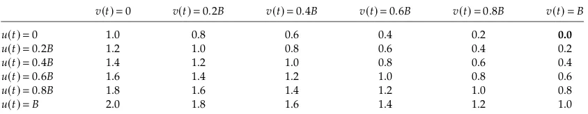
Table 1(a). Values ofτ0(t)
for Various Values ofu(t)andv(t), withγ−0.8
v(t)0 v(t)0.2B v(t)0.4B v(t)0.6B v(t)0.8B v(t)B
u(t)0 0.2 0.0 -0.2 -0.4 -0.6 -0.8
u(t)0.2B 0.4 0.2 0.0 -0.2 -0.4 -0.6
u(t)0.4B 0.6 0.4 0.2 0.0 -0.2 -0.4
u(t)0.6B 0.8 0.6 0.4 0.2 0.0 -0.2
u(t)0.8B 1.0 0.8 0.6 0.4 0.2 0.0
u(t)B 1.2 1.0 0.8 0.6 0.4 0.2
Table 1(b). Values ofτ0(
t)for Various Values ofu(t)andv(t), withγ−0.5
v(t)0 v(t)0.2B v(t)0.4B v(t)0.6B v(t)0.8B v(t)B
u(t)0 0.5 0.3 0.1 -0.1 -0.3 -0.5
u(t)0.2B 0.7 0.5 0.3 0.1 -0.1 -0.3
u(t)0.4B 0.9 0.7 0.5 0.3 0.1 -0.1
u(t)0.6B 1.1 0.9 0.7 0.5 0.3 0.1
u(t)0.8B 1.3 1.1 0.9 0.7 0.5 0.3
u(t)B 1.5 1.3 1.1 0.9 0.7 0.5
Table 1(c). Values ofτ0(
t)for Various Values ofu(t)andv(t), withγ−0.0
v(t)0 v(t)0.2B v(t)0.4B v(t)0.6B v(t)0.8B v(t)B
u(t)0 1.0 0.8 0.6 0.4 0.2 0.0
u(t)0.2B 1.2 1.0 0.8 0.6 0.4 0.2
u(t)0.4B 1.4 1.2 1.0 0.8 0.6 0.4
u(t)0.6B 1.6 1.4 1.2 1.0 0.8 0.6
u(t)0.8B 1.8 1.6 1.4 1.2 1.0 0.8
u(t)B 2.0 1.8 1.6 1.4 1.2 1.0
Note.Negative values ofτ0(
t)are shown in bold, to indicate that they violate FIFO.
we will measure the inflows and outflowsu(t)andv(t)
as fractionsk1andk2of the link capacityB, thusu(t)
k1Bandv(t)k2Bwhere 0≤k1≤1 and 0≤k2≤1. That
reduces the necessary and sufficient condition (23) to
τ0
(t)1+k
1−k2+γ >0. (24)
Tables 1(a) to 1(c) illustrate that the more negative is γ and/or the more rapidly x(t) is declining (it is
declining when the outflow ratev(t)exceeds the inflow
rate u(t)), then the more likely it is that FIFO is
vio-lated. Because k1 and k2 are nonnegative and do not
exceed 1, it follows from (24) thatτ0(
t)is always
posi-tive and therefore FIFO is always satisfied ifγ >0. In view of that, in Tables 1(a) to1(c), we consider only example values ofγ≤0, in particularγ−0.8,γ−0.5,
andγ0.
Tables1(a)and1(b)illustrate that when linear travel-time functions are inhomogeneous, as in (11), then FIFO violations can easily occur. This is in sharp con-trast to the behavior of linear homogeneous travel-time functions: each of the three papers discussed in Sec-tions3–5have shown that when the travel-time func-tions are linear and homogeneous then FIFO is always satisfied.
In the papers discussed in Sections 4 and 5, it is shown that part of the sufficient conditions for FIFO
derived for the nonlinear homogeneous travel-time models is that fx(x)<1/BwhereBis an upper bound
onu(t). In Sections4and5this is extended to nonlinear
inhomogeneous travel-time functions, so that the suffi-cient conditions for FIFO includefx(x,t)<1/BwhereB
is again an upper bound onu(t).
Now consider the second term before the “>0”
in (21), i.e., time fx(x(t),t)x0(
t). The term f
x(x(t),t)
is always nonnegative so we consider only the case when x0(
t) is negative, because that is the case that
is most constraining in the condition (21). Multiplying through fx(x(t),t)<1/Bbyx
0(
t)gives f
x(x(t),t)x 0(
t)> x0(
t)/B: note that the direction of the inequality is
reversed as a result of multiplying through by a nega-tive. Substitutingx0(
t)/Bfor f
x(x(t),t)x 0(
t)in (21) gives
τ0
(t)1+x0(t)/B+f
t(x(t),t)>0. (21’)
This is still a sufficient condition because fx(x(t),t) ·
x0(
t)>x0(
t)/B ensures that if (21’) is satisfied then so
is (21). Recall that x0(
t)u(t) −v(t) and substituting
this in (21’) and also assuming that f(x(t),t)takes the
separable form f(x(t))+γtso that f
t(x(t),t)γ, gives
τ0
(t)1+(u(t) −v(t))/B+γ >0. (21”)
This is the same form as (23) so we can again illustrate this in the same way as for (23). Recall that, to make
[image:10.612.92.523.91.178.2] [image:10.612.97.517.207.288.2] [image:10.612.96.518.315.397.2]the results illustrated in Tables1(a)–1(c)more general, we reduced the necessary and sufficient conditions for FIFO from (23) to (24) by measuring the inflows and outflowsu(t)andv(t)as fractionsk
1andk2of the link
capacityB. In the same way, and for the same reason, we reduce the necessary and sufficient FIFO condition (21”) to (24), by substituting u(t)k
1Bandv(t)k2B
into (21”). Thus Tables 1(a)–1(c) that illustrate FIFO adherence and violations for the linear inhomogeneous travel-time functions, also illustrate this for the nonlin-ear inhomogeneous travel-time functions.
Some simple examples of FIFO violations.
To further illustrate how a FIFO violation can occur for the travel-time models (1) and (3) it is useful to give some simple examples.
Example 1. An intuitive example of FIFO violations for the homogeneous case(1).We assume, as usual, that the travel-time function f(x(t)) is nondecreasing in x so
that fx(x(t)) is nonnegative hence, from (20), a FIFO
violation requires that x0(
t) u(t) −v(t) is negative
and of sufficient magnitude to ensure that fx(x(t)) ·
x0(
t) ≤ −1.
Suppose that the inflow u(t) and outflow v(t) are
positive, equal(u(t)v(t)), and constant leading up to
timetand suppose that the exogenous inflow rateu(t)
then starts decreasing rapidly. That does not affect the outflow ratev(t)until the inflow has traversed the link
to the exit, therefore the link occupancyx(t)decreases
at the same rate as u(t), which causes a decreasing
travel time f(x(t)). The latter will decrease faster if
the travel-time function is sloping steeply upwards (i.e., if fx(x(t))>0 is large) since, in that case, even
a small decrease inx(t)can produce a large decrease
in the travel time f(x(t)). In that case, the travel time
may decline so fast over time that the current vehicles may exit before preceding vehicles, which is a FIFO violation.
Two simple examples of FIFO violations for the inho-mogeneous case(3).
Example 2. Example1can easily be extended to allow
inhomogeneity over time, by assuming (3) rather
than (1), so that the FIFO condition is (21) rather than (20). From Example1, fx(x(t))x
0(
t) ≤ −1 becomes fx(x(t),t)x
0(
t) ≤ −1 so that the first two terms on the
l.h.s. of (21) become less than zero. If we let inhomo-geneity over time take the form of travel time declining over time for any givenx(i.e., time ft(x(t),t))then the
final term on the l.h.s. of (21) is also negative. In that case, the FIFO condition (21) is violated even more eas-ily than in Example1.
Example 3. Up to timet ort+τ(t)let the inflowu(t)
equal outflow v(t) so that x0(
t)u(t) −v(t)0 and
let ft(x(t),t)0, which reduces the l.h.s. of (21) to+1,
hence FIFO holds. Now suppose that from timetthere is inhomogeneity over time so that, for a given x, the travel time declines at a rate ft(x(t),t)<−1. In that case,
at time t the l.h.s. of (21) reduces to ft(x(t),t)<0 so
FIFO is violated.
8. Concluding Remarks
In dynamic traffic assignment modeling, a series of papers have treated the link travel times as functions of the number of the vehicles currently on the link. That is, for traffic entering at timetthe travel time is f(x(t))
where x(t) is the number of vehicles on the link at
timet. However, when this travel-time function is used to model traffic flows varying over time on a link it can violate a desirable first-in-first-out (FIFO) prop-erty. A number of papers have investigated this and other properties of the model and have derived condi-tions that are sufficient to ensure that these properties, including FIFO, will hold. The key sufficient condition is an upper bound on the gradient of f(x(t)), namely fx(x)<1/Bwhere Bis the upper bound on the entry
flow rateu(t).
In this paper we note that the link travel time can also vary directly with time, independently of the num-ber of vehicles on the link, so that the travel-time function becomes f(x(t),t). We derive conditions that
are sufficient to ensure that the properties, including FIFO, derived by earlier authors for the homogeneous travel-time function f(x(t))will also hold for the
inho-mogeneous travel-time function f(x(t),t). We retain
the conditions needed to ensure FIFO with respect to changes inx(t)and derive an additional condition that
will ensure FIFO when both arguments in f(x(t),t)
vary, i.e., x(t) and t both vary. We derive this
addi-tional condition first for linear travel-time functions, in Section3, by extending results from Friesz et al. (1993), and derive it for nonlinear travel-time functions, in Sec-tions 4–6, by extending results from Xu et al. (1999), Zhu and Marcotte (2000); and Carey and Ge (2005b), respectively.
For nonlinear travel-time functions the additional condition, that is sufficient to ensure FIFO, is a lower bound on the gradient ft(x,t), namely ft(x,t)>
−u(t)/B. For linear travel-time functions this
addi-tional condition reduces to ft(x,t)γ0(
t) ≥ −u(t)/B.
Both of these bounds show some similarity to the bound fx(x)<1/Balready derived, in the earlier papers
referred to in Sections2–6, for the case of travel-time functions f(x(t)). All of these conditions show that the
link inflows, and especially their upper boundB, play a major role in determining whether FIFO is ensured or not.
In Section 7 we give some examples of link travel-time functions varying over travel-time. We also give some numerical examples to illustrate when travel-time