Multiple sequence alignment algorithms for the phylogenic analysis of chloroplast DNA

(1)

Multiple sequence alignment

algorithms for the phylogenic analysis

of chloroplast DNA.

By

Adam Rumbold (BSc.)

A dissertation submitted to the

School of Computing

in partial fulfilment of the requirements for the degree of

Bachelor of Computing with Honours

University of Tasmania

(2)

Declaration

I, Adam Rumbold, declare that this thesis contains no material which has been accepted for the award of any other degree or diploma in any tertiary institution. To my knowledge and belief, this thesis contains no material previously published or written by another person except where due reference is made in the text of the thesis.

(3)

Abstract

The application of approximate string matching and alignment algorithms to either DNA or amino acid (protein) sequences is important for determining conserved regions, functional sites and to allow for multiple sequence alignments from which an evolutionary (phylogenic) tree may be inferred.

(4)

Acknowledgements

(5)

Table of Contents

Index of Tables

TABLE 1 TABLE OF CODONS AND THEIR TRANSCRIBED AMINO ACID...2

TABLE 2 GLOBAL AND LOCAL ALIGNMENT COMPARISON...5

TABLE 3 ALIGNING ALIGNMENTS EXAMPLE ...20

TABLE 4 COMPARISON OF SUBSTITUTION MODELS ...31

TABLE 5 MAJOR DNA DATABASES AND LOCATIONS...34

TABLE 6 MULTIPLE SEQUENCE ALIGNMENT ALGORITHMS ...36

TABLE 7 PHYLOGENIC PACKAGES...36

TABLE 8 SUMMARY OF THE PROCESSING AND MEMORY COMPLEXITY OF MSA APPLICATIONS ...47

TABLE 9 DESCRIPTIVE FEATURES OF THE ALIGNED MAIDENARIA DATA SET...50

(9)

Table of Figures

FIGURE 1 DYNAMIC PROGRAMMING MATRIX EXAMPLE...8 FIGURE 2 CHAOS ILLUSTRATION FROM (BRUDNO ET AL. 2003) ...12 FIGURE 3 MAVID MSA PROCEDURE FROM (BRAY & PACHTER 2004)...28 FIGURE 4 GROWTH OF THE NUCLEOTIDE DATABASES (NUMBER OF NUCLEOTIDES HELD) FROM JANUARY 1995 TO JANUARY 2004 ...35 FIGURE 5 DOT PLOT SHOWING THE INVERSION PRESENT IN OVATA919 AND

CRENULATA ALIGNMENT...45 FIGURE 6 DOT PLOT SHOWING THE INVERSION PRESENT IN GLOBHJ13CG9 AND

OVATA924 ALIGNMENT...45 FIGURE 7 EXAMPLE OF TRANSLOCATION REARRANGEMENT IN THE PAIRWISE

ALIGNMENT OF EGLOBULUS TASMANIANA1078 AND EBADJENSIS8001326...46 FIGURE 8 P-DISTANCE SCORES FOR ALL MSA...48 FIGURE 9 MSA ALGORITHMS (WITH SUBSTITUTION MATRIX) OF MAIDENARIA

DATA SET SHOWING ALIGNED LENGTH (BP) AND NUMBER OF INDELS...49 FIGURE 10 SUM OF PAIRS (SPS) SCORE AND WEIGHTED SUM OF PAIRS (W-SPS)

FOR ALL MSA ...51 FIGURE 11 UPGMA CONSENSUS TREE GENERATED FROM BENCHMARK ALIGNMENT

USING P-DISTANCE SUBSTITUTION MATRIX ...53 FIGURE 12 UPGMA CONSENSUS TREE GENERATED FROM ALIGNMENT

CONSTRUCTED USING AAE WITH NUCMATRIX USING THE P-DISTANCE

(10)

1. Introduction

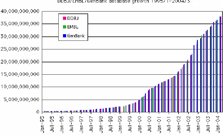
In recent years there has been an exponential increase in the amount of biological data being collected worldwide (see section 5.1). This wealth of data and the complexity of biological processes has nurtured a growing field of study in bioinformatics. Bioinformatics uses mathematical and informational techniques to solve biological problems, typically through computer programs or mathematical models. This research will focus on multiple sequence alignment techniques and their subsequent applications in inferring an evolutionary history (or phylogeny).

1.1 Biological Concepts

The cell is the basic structure of life and performs essential functions such as respiration, consuming nutrients and expelling metabolic waste. Within cells are DNA (deoxyribonucleic acid) molecules that ‘encode’ all the information necessary to produce the proteins essential to all cellular processes. It is for this reason that DNA is considered the ‘blue-print’ of life; and is recognised as distinguishing whether two living beings are biologically similar or distinct (Junior 2003).

The double helix structure of DNA was discovered by Crick and Watson in 1953. DNA consists of a double chain of simpler molecules called nucleotides. The nucleotides that comprise a strand of the double helix have a nitrogen base that can be of four types: adenine (A), cytosine (C), guanine (G) and thymine (T). These bases are the molecules that tie the double helix together. Each nucleotide consists of a sugar (eg deoxyribose in DNA), a phosphate and a base. The two strands comprising the double helix are complementary in the sense that adenine always bonds to thymine and cytosine always bonds to guanine. As such it is sufficient to know one strand to be able to deduce the other. The bonding between nucleotides form base pairs (bp), which is commonly used to specify DNA length.

(11)

1. Introduction

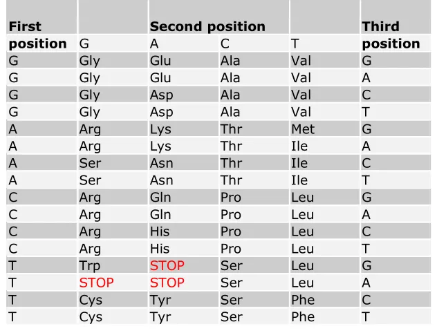
[image:11.612.178.494.237.478.2]

combination of 20 simpler molecules called amino acids. A sequence of three nucleotides (called a codon) code for a particular amino acid (see table 1), and the contiguous sequence of nucleotides that code for a particular protein is called a gene. In this sense a protein may be viewed as either a sequence of amino acids or equivalently a transcribed sequence of nucleotides that code for the specific amino acid sequence. The relationship between codons and amino acids is called the genetic code. Included in the genetic code are three special ‘STOP’ entries that indicate the end of a gene.

Table 1 Table of codons and their transcribed amino acid

Living organisms are made up of two types of cells prokaryote and eukaryote. Prokaryotes (eg bacteria) lack organelles (a structure with a specialised function) whilst most organisms including humans and plants are comprised of eukaryotic cells. “A eukaryotic cell has a nucleus, which is separated from the rest of the cell by a membrane. The nucleus contains chromosomes, which are the carriers of the genetic material- DNA. There are internal membrane enclosed compartments within eukaryotic cells, called organelles...which are specialised for particular biological processes.” (Lopez)

(12)

chloroplasts (for photosynthesis) and etioplasts (chloroplasts which have not been exposed to light).

1.2 Biological Sequences

DNA and protein sequences can be seen as long text strings over restricted alphabets. In the case of DNA there are four possible bases A, C, T and G that represent the alphabet, whilst amino acid sequences have an alphabet of 20 characters.

The comparison of two or more biological sequences can serve a number of purposes. Through the theory of evolution it is widely understood that gene sequences may have evolved from a common ancestral sequence. It is therefore of interest to study the evolutionary history of mutations (insertions and deltions of DNA as well as rearrangement mutations such as inversions and translocations) and other changes. The study of biological sequences can also be studied to locate regions of commonality, which may correspond to regions of similar structure or function.

The analysis of two or more sequences often occurs through the application of a sequence alignment algorithm and the measure of similarity that results. In aligning two or more sequences there are typically four possible operations that can be conducted on either sequence: insertion, deletion, substitution or transposition. In biology an insertion in one sequence can alternatively be seen as a deletion from the other. For this reason insertions or deletions are commonly referred to as indels. There are also a number of rearrangement events/mutations that can occur on biological sequences such as inversions (whereby a subsegment of DNA changes orientation), duplications (where a copy of a subsegment is inserted into the sequence), translocations (where a subsegment is removed and inserted in a different location) or a combination of the above.

(13)

1. Introduction

“They [SNP’s] are most commonly changes from one base to another - transitions and transversions - but single-base insertions and deletions (“indels”) are also SNP’s…Transitions change a purine to a purine or a pyrimidine to a pyrimidine – A to G or C to T and vice versa. Transversions change a purine to a pyrimidine and vice versa – A or G to C or T; C or T to A or G. Even though there are twice as many possible transversions as transitions, transitions tend to be at least equal to transversions in frequency, and often more prevalent.” (Gibson & Muse 2002)

1.3 Chloroplast DNA

Chloroplast DNA (cpDNA) is a coding region within plant cells, with many chloroplast DNA genes encoding proteins that are involved in photosynthesis. Depending on the species, chloroplast DNA has a size ranging from 110 000 bp to 160 000 bp (Blake). Samples of cpDNA have been useful in studies that take the geographic distribution of species into account when inferring an evolutionary history since cpDNA variation is correlated more with geographic distribution than with morphological species (Freeman et al. 2001). Chloroplast DNA is useful in studies because it is inherited maternally and is considered “a single, non-recombining unit of inheritance.” (Schaal et al. 1998)

1.4 Sequence Alignment

Sequence alignment and specifically multiple sequence alignment (MSA) is of fundamental importance within bioinformatics. By analysing the similarities and differences of either nucleotide or amino acid sequences it is possible to infer structural, functional or evolutionary relationships between the sequences being studied (Baxevanis & Ouellette 1998).

(14)

sequence alignment problem is to produce a pairing of characters from one sequence with the second sequence so that the total score is optimal. In pairing characters, gaps can be inserted at any position in the sequences; however the order of characters in each sequence must be preserved. A pairwise alignment is an alignment of two sequences and if there are more than two sequences the problem is called multiple sequence alignment (MSA).

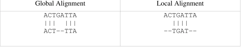
In aligning sequences there are two types of alignment: global and local. Global alignments attempt to align sequences over their entire length, whilst local alignments construct the best alignment of segments of the sequences that exhibit a high density of matches, ignoring the remaining regions of the sequences. Table 2 below shows examples of global and local alignments.

Global Alignment Local Alignment

[image:14.612.140.535.312.395.2]

ACTGATTA ||| ||| ACT--TTA

ACTGATTA |||| --TGAT--

Table 2 Global and local alignment comparison

Multiple sequence alignment algorithms are global however a number use local alignment algorithms to anchor the global alignment.

(15)

2. Sequence Alignment

2.1 Introduction

Approximate string matching has been an important tool in computational biology since small variations within DNA or protein sequences are common. Biologists often require searching the online databases with particular sequences so as to detect homologous sequences in other species. These searches allow biologist to analyse the similarities and differences of either nucleotide or amino acid sequences to aid in inferring structural, functional and/or evolutionary relationships between the sequences (Baxevanis & Ouellette 1998). It is also necessary to align sequences in the first stage of the process of creating phylogenic trees.

There is no such thing as a single best alignment with biological sequences since optimality always depends upon the assumptions made in the alignment algorithm such as the penalty ascribed to gaps or particular substitutions as well as the mutational events the algorithm is capable of handling. These decisions must be carefully considered according to the observed variations in the DNA or protein samples being considered (Baxevanis & Ouellette 1998). Furthermore, most sequence comparison methods use sequence alignment algorithms that inherently “assumes conservation of contiguity between homologous segments” (Vinga & Almeida 2003). This assumption is at odds with genetic recombination such as translocations and inversions. Stochastic modeling of sequences using hidden Markov models (Muckstein, Hofacker & Stadler 2002) and recently alignment-free sequence comparison methods (Vinga & Almeida 2003) are new techniques to overcome this.

2.2 Dot Plots

(16)

similarity globally and locally of the two sequences. That is global similarity is represented by a diagonal line from the top left to the bottom right of the dot-plot, whilst local similarity is shown by smaller diagonal lines within the dot-plot (Maizel & Lenk 1981). Dot plots of the data set examined are shown in section 7.1.

2.3 Sequence Alignment Techniques

Most formulations of sequence alignment consist of an objective function which assigns a score to each possible alignment of the sequences. The computational problem is to find an alignment which either optimizes the objective function through heuristic techniques, or guarantees an optimal score such as through a dynamic programming technique.

2.3.1 Dynamic Programming

Dynamic programming algorithms were initially developed to calculate the minimal edit distance between two sequences (Needleman & Wunsch 1970; Sellers 1974). The first dynamic programming algorithm to compute the edit distance and search for a pattern sequence within a text was developed by Sellers in 1980 (Sellers 1980). Many variations have been rediscovered and both theoretical and practical improvements have since been made (Chang & Lawler 1994; Chang & Marr 1994; Galil & Park 1990; Ukkonen 1985). These improvements have yielded an average case O( (kn)/ σ ) and worst case O(kn) algorithms (Navarro 2001), where σ is the size of the alphabet being considered and n is the size of the largest sequence.

Dynamic programming algorithms are particularly flexible in handling different distance functions, although they are not the most efficient algorithms in general. Dynamic programming routines guarantee the mathematically optimal alignment, and can easily be generalised to optimally align N sequences, however they process in O(LN_{) time where L is the length of the longest sequence and hence are}

(17)

and B, we first introduce the notation D(i,j) to represent the edit distance between the first i characters of A and the first j characters of B. The minimal edit distance of A and B (as defined in section 3.1) is D(n,m) and is calculated by first computing D(i,j) where i<n and j<m. This is achieved through the construction of a dynamic programming matrix and by a simple recurrence (Gusfield 1999).

The edit-distance metric scores a 1 for each mismatch or inserted gap and a 0 for a match. To calculate the optimal alignment of A and B (using the simple edit-distance metric) a matrix D0..n, 0..m is first constructed, where each element Di,j

represents D(i,j) and Dn,m represents the minimum edit distance between A and B.

The matrix is firstly initialised such that Di, o = i and D0, j = j since this represents

the edit distance between strings of length i or j respectively and the empty string which is equivalent to i/j deletions from the non-empty string. Then all the matrix values are calculated according to the formula:

Di, j= min(Di-1 , j-1 + d(Ai, Bj) , Di-1 , j +1 , Di , j-1 +1) where d(Ai, Bj) is 1 if Ai Bj

and 0 otherwise.

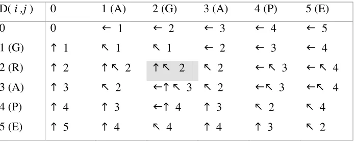
To find the optimal global alignment requires a traceback through the matrix, and to achieve this it is necessary to know the path by which each new value in the matrix was calculated. That is, in finding Di, j , we also store a pointer to cell Di-1, j if Di-1 , j

+1 was minimal, and/or a pointer to cell Di, j-1 if Di , j-1 +1 was minimal and/or a

pointer to cell Di-1, j-1 if Di-1 , j-1 + d(Ai ,Bj) was minimal. By storing pointers

indicating the direction from which the minimal value(s) were found an optimal alignment can simply be found through following any path from Dn m to D0,0 .

D( i ,j ) 0 1 (A) 2 (G) 3 (A) 4 (P) 5 (E)

0 0 1 2 3 4 5

1 (G) 1 1 1 2 3 4

2 (R) 2 2 2 2 3 4

3 (A) 3 2 3 2 3 4

4 (P) 4 3 4 3 2 4

[image:17.612.146.493.553.692.2]

5 (E) 5 4 4 4 3 2

(18)

In the above example (figure 1) the edit distance between “GRAPE” and “AGAPE” is found to be two and to find the optimal alignment a traversal back through the matrix following the direction of the pointers. When cell (2,2) is reached a choice between two optimal alignments must be made (either a substitution of G to R or a deletion of “R” from “GRAPE”. The two possible global alignments of the two sequences is shown below, both have an edit distance of 2:

Unaligned Aligned

AGAPE AG-APE AGAPE

GRAPE -GRAPE GRAPE

The above method can be easily altered to find localised regions of similarity by allowing for sequences that match the pattern to begin anywhere within the text. A locally matching region is found by selecting those areas within the matrix where the score is above some similarity threshold. The basic routine outlined above can also be easily extended to handle various other distance functions (include affine-gap penalties where the penalty ascribed to x insertion or deletions is given by a γ +

λx where γ is the gap-initiation cost and λ is the gap-extension cost).

2.3.2 Anchoring

Anchoring methods make use of a local alignment algorithm to first find regions of high similarity within the sequences, and then solve the problem of finding the best chain of the local alignments around which a global alignment is fixed. A local alignment can be represented by a series of diagonal pointers in the dynamic programming matrix. To chain two local alignments we require that a monotonic conservation map can be created. That is, if local alignment A is defined by (x1A , y1A) and (x2A , y2A) and local alignment B is defined by co-ordinates (x1B , y1B) and

(19)

There are a number of global pair-wise alignment algorithms which chain together regions of high similarity such as CHAOS, BLAST and LAGAN, as well as multiple sequence alignment algorithms DiAlign and Mavid.

2.4 Sequence Alignment Algorithms

2.4.1 NEEDLEMAN-WUNSCH

The Needleman-Wunsch (NW) algorithm (Needleman & Wunsch 1970) was the first algorithm to determine an optimal global alignment of two sequences. The algorithm developed a dynamic programming approach to calculating the mathematically optimal alignment over all residues of the sequences.

The original method is rarely used due to its cubic runtime (Gusfield 1999, p. 234), however through numerous improvements the run time has been improved (see section 2.3.1).

2.4.2 CHAOS (Chain of Scores)

The CHAOS algorithm (Brudno et al. 2003) is a heuristic local alignment algorithm that builds a global alignment using a set of local alignments called anchor points. CHAOS can be used as a stand-alone local sequence alignment program or as a pre-processing step for a global alignment algorithm (eg LAGAN, SLAGAN).

The algorithm works by chaining seeds – a pair of words of length k that has at least

n identical characters. Two seeds, s1 and s2 can be linked together if: the indices of s1 are higher than those of s2 in both sequences and the two seeds are ‘near’ to each

other. Two seeds satisfy this second condition if they are within a region defined by a gap score and distance cut-off, as illustrated in figure 2.

(20)

representing the string w1..wp also store back-pointers to the node containing the

string w2..wp.

The algorithm begins by inserting all of the k-mers of one sequence (database sequence) into the T-trie. The root of the T-trie is made the current node, and for every letter of the other (query) sequence:

1. If the current node has a child node corresponding to the letter under consideration this node is made the current node and any seeds stored in it are returned.

2. Otherwise make the node pointed to by the back-pointer the current node and return to step 1.

To keep a track of the available seeds to chain to, a probabilistic data structure called a skip list is used. A distance, D, specifies the maximal distance for which two seeds must be under to be chained together (see figure 2). Any seeds generated whilst examining the last D base pairs of the query sequence are stored in the skip-list. The seeds are ordered by the difference of its indices in the two sequences (diagonal number). For each seed s found at the current location, its diagonal number is found and a search of the skip-list is made to find any seeds in the skip-list whose diagonal number is within the allowable gap cut-off. This finds all possible previous seeds that s can be chained to, and the highest scoring chain is chosen.

(21)

[image:21.612.216.456.71.364.2]

Figure 2 CHAOS illustration from (Brudno et al. 2003)

2.4.3 LAGAN

Limited Area Global Alignment of Nucleotides — Lagan — is a fast heuristic pairwise alignment algorithm developed by Michael Brudno (Brudno et al. 2003). The algorithm first uses the CHAOS algorithm to find the set of all local alignments. These alignments are then weighted and the optimal chain (based upon the longest increasing subsequence algorithm) is chosen, with each local alignment in this chain an anchor to the global alignment. LAGAN then calls CHAOS recursively between two anchors when they are more than a threshold apart to overcome sparse regions. A Needleman-Wunsch like global alignment algorithm is then called in the areas between two anchors, and in a restricted area surrounding the anchors (ie. those cells within a distance of r from the anchor).

LAGAN uses memory proportional to the largest area between two local alignments plus the memory needed to hold the alignment (Brudno et al. 2004).

(22)

2.4.4 SLAGAN

(23)

3. Multiple Sequence Alignment

3.1 Introduction

All MSA algorithms require an objective function to determine the relative quality of each possible multiple sequence alignment. The sum-of-pairs (SP) objective function scores a MSA by the sum of the induced pair-wise alignments. For

example, considering the following simple MSA:

A: ACT-GGT B: -CTGGGT C: CCTGG-T

This alignment induces the following pair-wise alignments

A: ACT-GGT B: -CTGGGT

A: ACT-GGT C: CCTGG-T

B: -CTGGGT C: CCTGG-T

The sum of pairs objective function then scores the MSA M as S(M) = k<ls(k,l)

where s(k,l) is the pair-wise score of sequences k and l from MSA M. If a guide tree is known the weighted sum of pairs may be used to down-weight induced alignments which are less related than those closely related.

(24)

Multiple sequence alignment (MSA) algorithms can be classified into three classes: iterative, progressive and exact. The most widely used heuristic algorithms are based on the progressive alignment of sequences to create a multiple sequence alignment (Vision & McLysaght 2004). Typically however, expert knowledge is needed to review and for manual editing of a MSA to produce a ‘good’ alignment (Baxevanis & Ouellette 1998, p. 173; Thompson, J., Higgins & Gibson 1994).

A list of MSA applications is provided in section 5.2.2

3.2 Concepts

Progressive alignment methods are the most commonly used and have the advantage of speed and simplicity (Notredame 2002). Progressive alignment successively aligns pairs of sequences using pairwise alignment algorithms (such as Needleman-Wunsch etc). Progressive alignment algorithms differ in several key ways: the way they choose the order in which to do the alignment, if they involve the alignment of a single sequence to a single growing alignment or if subfamilies are built up leading to alignments of alignments, and the method of aligning and scoring sequences or alignments against existing alignments. The most important heuristic used in progressive alignment algorithms is to align the most similar sequences first (those with the smallest edit distance). Progressive sequence alignment algorithms are sensitive to the order of the pairwise alignments which is determined solely by alignments of only two sequences at a time (Morgenstern, Dress & Wener 1996). This has been addressed recently by using a travelling salesman approach to determine the order of alignments (Chantal & Gaston 1999).

(25)

Iterative methods produce a MSA and then refine the alignment through stochastic or deterministic iterations (or cycles). Hidden Markov Models, and other statistically-based methods, have been used to attempt to associate a probability value to an alignment, and to encapsulate some of the known evolutionary information into the MSA.

3.3 Multiple Sequence Alignment Algorithms

3.3.1 Aligning Alignments Exactly

Kececioglu and Starret (Kececioglu & Starrett 2004) recently published the first algorithm to align alignments exactly (AAE) using linear gap costs and under the sum of pairs objective function. “Aligning Alignments is the problem of finding an optimal alignment of the columns of two multiple sequence alignments under the sum-of-pairs objective with linear gap-costs. The sum-of-pairs objective scores a multiple alignment by the sum of the scores of the two-sequence alignments induced on all pairs of sequences. With linear gap-costs a run of either x insertions or deletions costs γ + λx where γ is the gap-initiation cost and λ is the gap-extension cost.”(Kececioglu & Starrett 2004) Although an NP-complete problem, the algorithm was published with a number of speed-ups leading to a linear run time.

The algorithm is based upon a dynamic programming routine where each alignment is treated as a sequence of columns. When aligning an alignment A of k rows and m

columns to an alignment B of l rows and n columns an m+1 by n+1 grid structured graph is constructed. The graph is traversed in row-major order until the final cell (m,n) has been calculated. Costs within the dynamic programming table are calculated according to the cost of composing a column to the current alignment.

(26)

character last. That is, row 3 underhangs rows 0,1 and 2, whilst row 0 overhangs

row 3 in the alignment. Each cell in the table can have a number of shapes and corresponding scores for the optimal alignment ending in that shape.

The column to be added to the current alignment is determined through the position in the table and the direction of the cell under consideration. If we let the set of shapes at a particular entry (i, j) in the table be denoted by S(i,j). When at position (i, j) in the dynamic programming table and considering shape s ∈ S(i, j) the calculation of the score at the adjacent cells is detailed below:

(i, j+1) = The cost of composing a column consisting of gaps in alignment A and characters from column j+1 in alignment B to the shape s.

(i+1, j) = The cost of composing a column of characters from column i+1 in alignment A and gaps in alignment B to the shape s.

(i+1 , j+1) = The cost of composing a column of characters from column i+1 in alignment A and characters from column j+1 in alignment B to the shape s.

Using the following notation:

A[i, j] = the character at row i and column j of alignment A A[j] = column j from alignment A

S(i ,j) = the set of shapes at entry (i, j) in the dynamic programming table

C(i, j, s) = the cost of the alignment of prefixes A[1:i] and B[1:j] that ends in shape s.

S(i,j)o c = the set of shapes obtained by composing column c to the set of shapes S(i,j) .

(27)

(

)

(

)

−

∪

−

∪

−

=

+

=

otherwise

j

B

i

A

o

j

i

S

j

B

o

j

i

S

i

A

o

j

i

S

j

i

l

k

j

i

S

]),

[

],

[

(

)

1 ,

1 (

])

[

,

(

)

1 ,

(

)

],

[

(

)

,

1 (

0 &

0 ,

,...,

1 ,

,...,

1 )

,

(

To count the number of gaps initiated the following notation is introduced. For rows p and q in an alignment of shape s and column c:

• qsp if, and only if, p overhangs q in the alignment

• p_s

q if, and only if, p underhangs q in the alignment

• qcp if, and only if, p has a letter and q has a gap in column c

• p_c

q if, and only if, q has a letter and p has a gap in column c

Using the notation (a,b) to denote a column where a is either a column from alignment A or a column of gaps(‘-‘) and b is either a column from alignment B or a column of gaps. The total number of gaps initiated by composing a column (a,b) onto an alignment that has shape s is:

∈∈

=

B qp A

q p q p p q p

q

a

b

s

a

b

s

b

a

g

(

,

)

((

(

,

)

&

)

||(

(

,

)

&

)

where denotes logical negation (NOT), || denotes logical OR and the & denotes logical AND. In the above summation a true value maps to 1 and false maps to 0.

(28)

∈∈ = − − ∈ = − − ∈ = − − ∈ B qp A t

j B i A

soSi j

s

t j B soSi j s

t i A

soSi j

s

i

q

B

i

p

A

s

j

B

i

A

g

s

j

i

C

j

B

k

s

j

B

g

s

j

i

C

i

A

l

s

i

A

g

s

j

i

C

t

j

i

C

])

,

[

],

,

[

(

)

],

[

],

[

(

)

,1

(

min

]

[

)

],

[

,

(

)

,1

,

(

min

]

[

)

,

],

[

(

)

,

1 (

min

)

,

(

]) [ ], [ (( 1, 1)

]) [ , ((, 1)

) ], [ (( 1, )

Where |c| is the number of characters in the column, and a,b is the substitution cost for a match/mismatch of a character a from alignment A with a character b

from alignment B.

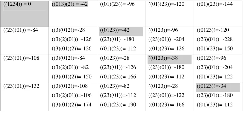
To illustrate the basic principles of the algorithm consider the following example of aligning two alignments of two sequences each:

Sequence number Alignment A Sequence number Alignment B

0 ATG 2 ACTG

1 ATG 3 -CTG

(29)

((1234)) = 0 ((013)(2)) = -42 ((01)(23))= -96 ((01)(23))=-120 ((01)(23))=-144

((23)(01)) =-84 ((3)(012))=-28 ((3)(2)(01))=-126 ((3)(01)(2))=-126 ((0123))=-42 ((23)(01)=-180 ((01)(23))=-112 ((0123))=-96 ((23)(01))=-204 ((01)(23))=-126 ((0123))=-120 ((23)(01))=-228 ((01)(23))=-150 ((23)(01))=-108 ((3)(012))=-84

((3)(2)(01))=-82 ((3)(01)(2))=-150 ((0123))=-28 ((23)(01))=-126 ((01)(23))=-166 ((0123))=-38 ((23)(01))=-180 ((01)(23))=-112 ((0123))=-96 ((23)(01))=-204 ((01)(23))=-122 ((23)(01))=-132 ((3)(012))=-108

[image:29.612.140.546.85.276.2]

((3)(2)(01))=-106 ((3)(01)(2))=-174 ((0123))=-82 ((23)(01))=-112 ((01)(23))=-190 ((0123))=-28 ((23)(01))=-122 ((01)(23))=-166 ((0123))=-34 ((23)(01))=-180 ((01)(23))=-112

Table 3 Aligning Alignments example

The optimal alignment is then constructed through a traceback procedure similar to that used in the NW dynamic programming algorithm. The shape with the highest score at cell (m,n) is first selected (see shaded cell at position (3,4) ). The corresponding shape ((0123)) indicates that characters from both alignment A and B are in the final column of this alignment. This, in-turn, indicates that a substitution column must have been composed to give this shape and score. Consequently a move to cell (m-1, n-1) can be made (ie. back one column in each alignment to cell (2,3) ). From cell (2,3) we consider all shapes in S(2,3) and determine the shape which under composition of a substitution column (A[3],B[4]) gives a score of -34. This calculation yields shape ((0123)) of score -38. This process continues until the cell (0,1) is reached where the shape is ((013)(2)). This shape indicates that only row 2 has a character in the final column and hence that gaps must have been inserted in alignment A (rows 0 and 1). This brings us to the original cell (0,0).

By following the path through the table and using the direction and positions in the table to determine the column of composition the optimal alignment is constructed as shown below.

(30)

The processing time and memory requirements are dependant upon the number of shapes, which in turn is dependant upon the gap structure of each alignment. Kececioglu and Starret developed two techniques (dominance pruning and bound pruning) which reduce the number of shapes added to the dynamic programming table. Bound pruning is very effective, with a large proportion of the table containing empty shape lists (Kececioglu & Starrett 2004).

3.3.2 Partial Order Alignment

A directed acyclic graph (DAG) representation of aligned sequences using a partial order graph has allowed for the development of an efficient alignment algorithm called Partial Order Alignment (POA) (Lee, Grasso & Mark 2002).

During progressive multiple sequence alignment algorithms there is the problem of incorrect scoring due to artifactual gap counts. When constructing a MSA through aligning a sequence to the current MSA, the MSA is first reduced to a consensus sequence or profile. This reduction results in a loss of information which inturn can lead to incorrect gap costs.

Artifactual gap counts are a legacy of aligning a sequence(s) to the profile of an alignment as illustrated in the simple example adapted from Lee et. al (Lee, Grasso & Mark 2002) below:

Consider the sequences:

A) TGACTCGATATATCG

B) CAGTCCGATAAGTCGTATCG

C) CAGTCCGATAAGTCGTATCG

A possible global alignment of sequences A and B is shown below, with its corresponding profile sequence (with sequence C shaded along its length):

(31)

profile 1:

CAGTCTGACTCGATAAGTCGTATCG

The problem of artifactual gap costs can be seen when examining the gaps in the two shaded columns of the alignment, and the effect of adding sequence C to this current alignment. Whilst the gap above the ^ is a true gap, the gap above the * is an artefact of the alignment, as another equivalent alignment demonstrates:

Alignment 2:

TGACT---CGATA---TATCG ---CAGTCCGATAAGTCGTATCG profile 2:

TGACTCAGTCCGATAAGTCGTATCG

If sequence C was aligned to alignment 1 there would be a 5 residue gap penalty, however this does not occur in alignment 2.

The partial order alignment represents alignments 1 and 2 as the same partial order graph. Sequence A and B are represented as a graph in a process shown below adapted from Lee et. al (Lee, Grasso & Mark 2002):

a) The standard row-column representation of the sequence alignment

TGACT---CGATA---TATCG ---CAGTCCGATAAGTCGTATCG

b) Each sequence is represented as a linear graph with each character a node and the order preserved.

T G A C T C G A T A T A T C G

(32)

T G A C T

C G A T A



>T A T C G

C A G T C A G T C G

The MSA using POA algorithm is essentially a progressive dynamic programming algorithm. The algorithm uses a standard Needleman-Wunsch routine, however instead of aligning a profile sequence to another sequence, the partial order (alignment) is used. To cope with multiple sequences without going into an N dimensional space each bifurcation in the graph structure becomes another dynamic programming plane whose cells must be considered when tracing back through the grid to determine the optimal alignment.

3.3.3 ClustalW

ClustalW (Thompson, J., Higgins & Gibson 1994) is a progressive multiple sequence alignment algorithm that improves the sensitivity through selective weighting of sequences and substitution scores. ClustalW performs a pairwise alignment on all the sequences in order to construct a binary tree of their evolutionary relationship. This is then used to build a MSA by aligning the most recently diverged sequences first. ClustalW creates N/2 alignment profiles, which are then aligned to each other resulting in N/4 profiles. This process is continued until all the sequences have been aligned.

(33)

in an attempt minimise the dependance on the choice of weight matrix. Closely related sequences (based on the percentage identity score) use a higher GOP, with less similar sequences having a linearly reducing GOP. Longer sequences increase the alignment scores, so the GOP is logarithmically scaled based on the length of the shorter sequence being aligned. These three factors alter the GOP so that for sequences of length N and M:

GOP = {GOP+log[min(N,M)}*(average residue mismatch score)*(% identity scaling factor)

The gap extension penalty - GEP, is modified according to the difference in lengths of the two sequences. If there is a large difference in lengths of the two sequences, then the GEP is increased to limit the number of long gaps in the shorter sequence. So that:

GEP = GEP*[1.0+ |log(N/M)|]

The GOP and GEP are also then altered throughout the alignment procedure depending upon the position. If there is a gap at a position then the GOP and GEP are lowered so that:

GOP = GOP*0.3*(number of sequences without a gap / no of sequences) GEP = GEP*0.5

If the position being considered does not contain any gaps but a gap is within 8 positions then the GOP is increased so that:

GOP = GOP*{2 + [(8- distance from gap)*2]/8}

(34)

3.3.4 DiAlign

DiAlign (Morgenstern 1999; Morgenstern, Dress & Wener 1996) is an anchor based algorithm that works by aligning gap-free segments of variable lengths from both sequences. The segments under comparison appear as a diagonal on a dot-plot, and are the basis of the diagonal alignment – DiAlign algorithm.

To compute the best alignment, DiAlign finds the maximal scoring set of consistent diagonals. Diagonals D1 and D2 are consistent diagonals if the positions (residues)

aligned to each other in D1 precede those aligned in D2, or vice-versa (see section

2.3.2). To determine the significance of a diagonal the following formulae are used:

For a fixed diagonal D, of length l and containing m matches, with p the probability of a point in the dot plot (ie. 0.25 for nucleic acids).

( )

p

l i

l m i i i l m l

P

−

=

1

) ,

(

Then using the negative logarithm, the weighting of D is defined as:

otherwise T m l E m l P D w , 0 ) , ( )), , ( ln( ) (

A high scoring weight indicates that a random diagonal of length l is unlikely to contain as many as m matches by chance. DiAlign scores highly for short segments with a large number of matches or for longer segments with fewer matches, so long as the segment is long enough.

For a set of diagonal D1, D2, D3,…, Dk the score is defined as:

score(i, j) :=

= k i i D w 1 ) ( . and

prec(i, j) :=Dk = − − < = −

(35)

A consistent set of diagonals with a maximum score is a maximum alignment. The maximum alignment of two sequences is then calculated using a dynamic programming algorithm based upon maximising the score of the alignment of prefixes of both sequences. This is achieved through the following definitions and recurrences:

(D) := the maximum sum of weights up to and including diagonal D (D must have a positive weight).

(D) := the diagonal preceding D.

score(i, j) := the score of the maximum alignment of A 1…i and B1..j

So, (D) = score (i-k-1, j-k-1) + w(D) and (D) = prec(i-k-1, j-k-1)

Now a recursive formulation of the score is given by:

score(i, j) =max{score(i ,j-1) , score(i-1, j) , (Di,j) } , where Di,j is any diagonal

ending at point (i, j) that satisfies (Di,j) = max{ (D): D ends at point (i, j)}.

To generalise DiAlign to N sequences “…we try to select a consistent set of diagonals with a maximal sum of weights. However, now diagonals originate from all the 1/2N(N-1) possible pairwise sequence comparisons.”(Morgenstern, Dress & Wener 1996). DiAlign sorts diagonals according to their weights, irrespective of which sequence the diagonal originates from. The set of all diagonals from all the maximal pairwise alignments is sorted by weights and the overlap score (favouring diagonals that occur over multiple sequences), and diagonals are added individually in order to the multiple alignment so long as the diagonal being considered is consistent.

(36)

3.3.5 Mavid

Mavid is a progressive global multiple alignment algorithm based upon the alignment algorithm AVID (Bray, Dubchak & Pachter 2002) and using maximum likelihood phylogenic techniques.

The sequences to be aligned are first aligned in a pairwise manner to produce a guide tree. This guide tree is used to determine the order in which sequences are aligned. The key difference in the MAVID algorithm to other progressive alignment algorithms is that instead of aligning two alignments directly through a consensus sequence, MAVID firstly infers ancestral sequences using standard phylogenetic models and then uses the alignment of these ancestral sequences using AVID to dictate the actual alignment.

(37)

[image:37.612.150.518.69.305.2]

(38)

4. Phylogenic Reconstruction

‘This is a huge, complicated, and highly contentious field. However, always remember that regardless of algorithm used, parsimony, any distance method, maximum likelihood, or even Bayesian techniques, all molecular sequence phylogenetic inference programs make the absolute validity of your input alignment their first and most critical assumption. The accuracy of your alignment is the most important factor in inferring reliable phylogenies; the results are utterly dependent on its quality.’(Thompson, S. M. 2004, p. 11)

4.1 Introduction

Phylogeny is the field of biology that is concerned with identifying and understanding the relationship between species based on ancestor/descendant relationships. The phylogeny of organisms is usually represented by an evolutionary tree (or a cladogram).

Phylogeography is the study of the relationship between the phylogenic variations within or between species and their geographic distribution. Chloroplast DNA is particularly appropriate for phylogeographic studies since cpDNA does not recombine and inheritance is mostly maternal (Freeman et al. 2001).

Phylogenetic analysis of DNA or amino acid sequences involves four steps: sequence alignment, determination of the substitution model, tree building and tree evaluation (Baxevanis & Ouellette 1998).

(39)

4. Phylogenic Reconstruction

The tree building criteria has an effect upon the alignment and substitution models applied. There are three tree building criteria used for calculating the phylogeny: distance matrix, maximum parsimony (MP) and maximum likelihood (ML).

“Distance trees use pairwise divergence estimates of all sequences in the data to determine tree topology and branch lengths. Maximum parsimony finds the tree that explains with the fewest number of discrete steps all the base differences in a multiple sequence alignment. Maximum likelihood finds the topology and branch lengths that have the highest probability of producing the observed multiple sequence alignment.” (Baxevanis & Ouellette 1998, p. 191)

For even moderate numbers of sequences being analysed there is an exponentially large number of possible trees for which the ‘best’ representation of the evolutionary relationship must be selected. As a result the optimal phylogenic tree(s) may only be found when examining generally fewer than 11 species. When the number of sequences being analysed exceeds 11 but is less than approximately 20, branch-and-bound methods can be used to find optimal phylogenic trees. For larger data sets most tree estimates are found using an uphill searching algorithm. Uphill searching heuristics are employed in the common phylogenic software packages PAUP (Swoffard 1998) and Phyllip (Felsenstein 1993) (Salter 2000).

4.2 Substitution Models

(40)

between the different substitutions and the frequency of the target base. (Baxevanis & Ouellette 1998, pp. 189-230)

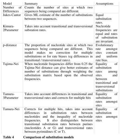
There are numerous available substitution models as summarised in the table below (further details of the substitution models can be seen in appendix A).

Model Summary Assumptions

Number of

Differences Counts the number of sites at which two sequences being compared are different. Jukes-Cantor Gives ML estimate of the number of substitutions

between two sequences. Equal substitution

rates.

Kimura-2Parameter Takes into account transitional and transversional substation rates. Nucleotide frequencies are equal and rates of substitution are invariant. p-distance The proportion of nucleotide sites at which two

sequences being compared are different. This model makes no correction for multiple substitutions or for rate biases (eg differences in transitional / transversional rates).

Evolutionary rate amongst sites constant and uniform rate bias. Tajima-Nei When nucleotide frequencies differ from 0.25 the

Tajima-Nei distance can give better estimates of number of substitutions through weighting the substitution matrix based upon the observed frequencies.

Equality of substitution rates among

sites and

between

transitional and transversional substitutions

Tamura-3Parameter Takes into account differences in transitional and transversional rates and corrects for multiple hits Equality substitution of rates amongst sites

Tamura-Nei Corrects for multiple hits, takes into account differences in substitution rates between nucleotides and the inequality of nucleotide frequencies. It also distinguishes between transitional substitution rates between purines (nucleotides A or G) and transversional rates between pyrimidines (C or T).

[image:40.612.136.536.168.630.2]

Equality of substitution rates amongst sites

(41)

4. Phylogenic Reconstruction

4.3 Tree Building

Many tree building methods have been developed, including: branch-and-bound, branch swapping, star-decomposition, divide-and-conquer and stochastic search methods (such as simulated annealing, genetic algorithms or Markov Chain Monte Carlo methods). One of the most widespread tree building methods is a form of star decomposition called neighbour-joining (Saitou & Nei 1987) which uses a distance matrix criteria. This method has also been adapted for MP and ML criteria (Bruno, Socci & Halpern 2000; Yang 1997).

For n species or sequences under consideration there is:

)!| 2 ( |

)! 5 2 (

2

−3

n n

n possible unrooted trees, with an even greater number of possible

trees for rooted trees. The methods employed to infer relationships and degree of divergence between sequences is beyond the scope of this study as it is a significant area of research in itself.

4.4 Tree Evaluation

Tree evaluation methods include: skewness test (randomised trees), permutation tests (randomised character data), resampling (bootstrapping, parametric bootstrapping, jackknife) and likelihood ratio tests. (Baxevanis & Ouellette 1998, pp. 213-7)

(42)

(43)

5. Bioinformatics Resources

“The computational biology community in general has been very generous with the fruits of its labour, making freely accessible tools and specialized databases without which elementary sequence analysis could not take place.” (Baxevanis & Ouellette 1998)

Bioinformatics is a recent and fast moving field. There is currently a myriad of available software packages and online references. This chapter shall note some of the most commonly used packages, languages and websites for those looking at analysing DNA sequences.

5.1 Online Databases

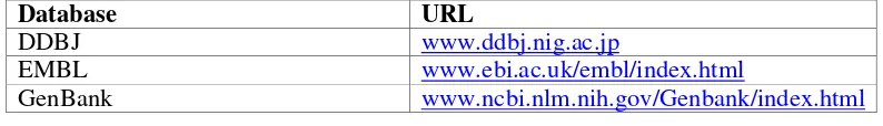
The International Nucleotide Sequence Database Collaboration (INSDC) maintains the major DNA sequence databases. INSDC is comprised of the DNA Data Bank of Japan (DDBJ Homology Search System), the European Molecular Biology Laboratory Nucleotide Sequence Database and the NCBI operated Genbank (see table 5 below). These databases collaborate to share new submissions and as such are synonymous although they do use different formats (Vision & McLysaght 2004).

Database URL

DDBJ www.ddbj.nig.ac.jp

EMBL www.ebi.ac.uk/embl/index.html

[image:43.612.138.535.491.548.2]

GenBank www.ncbi.nlm.nih.gov/Genbank/index.html

Table 5 Major DNA databases and locations

(44)

[image:44.612.146.532.73.308.2]

Figure 4 Growth of the nucleotide databases (number of nucleotides held) from January 1995 to January 2004

5.2 Software

Coupled with the databases listed above are many freely available online tools for searching the databases. One such collection of tools is ENTREZ which provides an entry point for many of the searching tools and resources provided by NCBI

Many of the tools used in analysing DNA and protein sequences are freely available and open source software. There are also programs available for conversion between sequence formats, for multiple sequence analysis and for phylogenic analysis (sections 5.2.1 and 5.2.2). A non-complete list of software available is included below.

5.2.1 Multiple Sequence Alignment

(45)

5. Bioinformatics Resources

Program Algorithm URL Reference

MSA Exact ftp://fastlink.nih.gov/pub/msa/ (Lipman, Altschul & Kececioglu 1989) DCA Exact

http://bibiserve.techfak.uni-biefeld.de/dca (Stoye, Moulton & Dress 1997) OMA Iterative DCA

http://bibiserve.techfak.uni-biefeld.de/oma (Reiner, Stoye & Will 2000) ClustalW Progressive ftp://ftp-igbmc.u-strasbg.fr/pub/clustalW (Thompson, J., Higgins

& Gibson 1994) MultAlin Progressive http://ww.toulouse.inra.fr/multalin.html (Corpet) DiAlign

Consistency-based http://www.gsf.de/biodv/dialign.html (Morgenstern, Dress & Wener 1996) ComAlign

Consistency-based http://www.daimi.au.df/ocaprani (Bucka-Lassen, Caprani & Hein 1999) T-Coffee

Consistency-based, Progressive

http://igs-server.cnrs-mrs.fr/~cnotred (Notredame, Holm & Higgins 1998)

IterAlign Iterative http://giotto.Stanford.edu/~luciano/iterali

gn.html (Brocchieri & Karlin 1998) SAM Iterative/Stoch

astic/HMM [email protected] (Hughey & Krogh 1996) HMMER Iterative/Stoch

astic/HMM http://hmmer.wustl.edu/ (Eddy 1995) SAGA Iterative/Stoch

astic/GA http://igs-server.cnrs-mrs.fr/~cnotred/ (Notredam & Higgins 1996) POA Partial order

alignment http://www.bioinformatics.ucla.edu/poa (Lee, Grasso & Mark 2002) GA Iterative/Stoch

astic/GA [email protected] (Zhang & Wong 1997)

Table 6 Multiple sequence alignment algorithms

5.2.2 Phylogenic Analysis

Some of the major phylogeny programs are shown below:

Application Criteria URL Operating System

PHYLIP MP &

ML http://evolution.genetics.washington.edu/phylip.html Windows, Mac, Unix PAUP http://paup.csit.fsu.edu/ Mac, Unix, Dos,

Windows

HYPHY ML http://www.hyphy.org/ Mac, Windows, Unix PAML ML http://abacus.gene.ucl.ac.uk/software/pa

ml.html Windows, Unix, Mac OSX, Linux

Table 7 Phylogenic packages

5.3 Programming

[image:45.612.139.530.76.427.2] [image:45.612.140.528.493.602.2]

(46)

supporting open source programming in bioinformatics. The Open Bioinformatics Foundation (O|B|F OPEN BIOINFORMATICS FOUNDATION) contains projects in BioPerl, BioJava, BioPython, BioRuby, BioPipe, BioSQL / OBDA, Moby and DAS. These projects include freely available methods and scripts to handle standard tasks such as file conversion and database searching amongst others.

(47)

6. Methodology

6.1 Aims

The JLA and an extended JLA+ region of cpDNA of eucalypts has been found to be

hypervariable (Freeman et al. 2001; Vaillancourt & Jackson 2000). The cpDNA sequences from these regions have been used to investigate the evolution and biogeography of eucalypts (Freeman et al. 2001; Whittock 2000). The high level of variation within the JLA+ region of E. globulus has led to difficulties in creating an

unambiguous alignment of the sequences for phylogenetic analysis. As a consequence sequences have been aligned by eye using Sequence Navigator software (Karplus K & Hu 2001; Whittock 2000). The treatment of gaps in constructing a multiple sequence alignment on such variable sequences is problematic. For this reason an exact multiple sequence alignment algorithm was implemented and compared with new and existing heuristic MSA algorithms.

The alignment generated by the biologist was used as a benchmark alignment to compare the MSA generated with POA, clustalW, MAVID, DiAlign and AAE. Descriptive features of these alignments were analysed along with other statistics detailed in section 6.4. Phylogenic trees were then constructed from the alignments and analysed for differences, and support (see section 6.5).

The analysis of cpDNA samples also aimed to identify inversions and other rearrangement mutations within the data set and to determine if inversions (if any) were having a detrimental effect upon the multiple sequence alignment.

(48)

6.2 Implementation

The raw data sequences obtained from plant science were of all samples of

Symphomytrus (71 species). The sequences were already aligned in the nexus file format. This format is used by PAUP and other programs and aims to be an extensible multiple sequence format. The Nexus file format contains a header block with information regarding the number of species, the aligned length and information on the types of sequences (DNA/Amino Acid) the gap character and the character for any missing data.

A number of Perl scripts were written to parse out the individual sequences from this file and remove all gaps so that the raw sequence data was available for analysis. This was achieved through Perls extensive regular expression functionality. Perl scripts were also written to analyse the alignments generated by SLAGAN and to parse out all alignments which contained inversions (see code snippet below).

if ($gdata =~ m/\-/){

print logf "found an inversion in: $filea\_$fileb \n"; @nums = ($gdata =~ m/(\d+\.?\d*|\.\d+)/g);

$x1 = $nums[1]; $y1 = $nums[2]; $x2 = $nums[8]; $y2 = $nums[9];

print logf "* $filea\_$fileb - between: \($x1 , $y1 ) \($x2 , $y2) ";

(49)

6. Methodology

A C G T - N A 91 -114 -31 -123 0 -43 C -114 100 -125 -31 0 -43 G -31 -125 100 -114 0 -43 T -123 -31 -114 91 0 -43 - 0 0 0 0 0 0 N -43 -43 -43 -43 0 -43

-750 -25

In the above substitution matrix (nucmatrix), substitutions between different DNA bases are prescribed different penalties, with matching DNA characters all scoring highly (either 100 or 91), the numbers in the final line of the matrix represent the gap open penalty (-750) and the gap extension penalty (-25). Most substitution matrices are developed for amino acid substitutions; with the exception of the above matrix as used in LAGAN (Brudno et al. 2003), the clustalW1.6 matrix and the IUB matrix (see Appendix A).

The AAE algorithm was implemented using modified sequence and multi-sequence objects developed by Brudno as a part of the LAGAN source code (licenced under GPL). The algorithm was implemented with the dominance pruning speedup and was capable of aligning all sequences in the maidenaria set. Descriptive features of the resultant alignment are shown in section 7.2 with the MSA shown in Appendix B.

6.3 Analysis of Inversions

(50)

conservation map. A list of the sequences for which inversions were found in the SLAGAN pairwise alignment was written to file.

The initial (21) pairwise alignments generated by clustalW based on the guide tree were examined to determine if inversions were present. The number and length of any inversions present give an indication of the extent to which inversions may hamper tradition MSA algorithms.

The results for detecting inversions is presented in section 7.1.

6.4 Analysis of Alignments for Phylogenic Reconstruction

Thompson et al. introduced two measures for comparing an alignment to a reference alignment: the sum of pairs score (SPS) and the column score (CS) (Thompson, J., Plewniak & Poch 1999). The SPS score increases as more sequences are correctly aligned and signifies the extent to which the algorithm succeeded in aligning the sequences in the alignment. The column score gives a measure of the ability of an algorithm to align all of the sequences correctly, however only one character in any column must be different causing a zero score. For this reason the CS was not used as a measure of how the generated alignments compared with the benchmark alignment

The SPS statistic used is the ratio of the all residue pairs that are aligned in the test alignment against the sum of all residue pairs in the reference alignment. That is, for an alignment A, of N sequences and M columns, and with column i from A represented as Ai1, Ai2, .. , AiN . Then defining pijk = 1 if residues Aij and Aik are

aligned. Then the score for the ith column Si is given by:

= ₌≠

= N_j N

kj k ijk

i

p

S

1 ₁

(51)

6. Methodology

=

= ÷

= M

SPS R

i Ri

M

i1

S

i 1

S

This formula allows for a comparison of the two MSA and the degree to which they have successfully aligned all the sequences. The above formula has also been modified to score 2 for identically aligned pairs of residues, a 1 for aligned gaps and 0 otherwise (Karplus K & Hu 2001). This scoring has been called the weighted sum of pairs score (W-SPS).

Most MSA programs aim to maximise an objective function however when analysing constructed alignments against verified alignments (such as those in BaliBase test suite) often the weighted sum of pairs score is higher in the test alignments than the ‘true’ alignment (Lassman Timo & Erik 2002, p. 127).

In using a MSA for phylogenic analysis each column and the variations within it are considered, and as such, those columns which contain the same character over all sequences are uninformative. Maximum parsimony methods of constructing an evolutionary tree include only those sites which exhibit at least two different nucleotides, and for which those nucleotides occur at least twice, in its analysis. For this reason examining the percentage of parsimony informative sites over an entire MSA enables a comparison of the informative content of each MSA in creating an evolutionary tree using MP methods.

The percentage of singleton sites was scored. A singleton site is a site containing at least two types of nucleotides; with at most one occurring multiple times. Constant sites are sites for which there is only one nucleotide occurring over all the sequences. The percentage of constant sites was scored, along with the percentage of variable sites. A variable site is either parsimony informative or a singleton site and as such all sites are either variable or constant.

(52)

compared are different. The p-distance is calculated by dividing the number of differences found by the total number of nucleotides compared and is averaged by the number of sequences.

The following multiple sequence alignment programs were used in the comparison: POA, ClustalW, Aligning Alignments Exactly, DiAlign and MAVID along with a number of substitution matrices. A table of the descriptive features of these alignments is presented in section 7.2.2. The speed, space complexity and other advantages/disadvantages of the aforementioned algorithms are detailed in section 7.2.1.

6.5 Phylogenic Analysis

(53)

7. Results and Discussion

7.1 Rearrangement Mutations

Due to the hypervariable nature of the chloroplast DNA samples it was decided to use the SLAGAN algorithm to detect inversions and determine if these inversions (if any) were having a detrimental impact on the MSA. Using SLAGAN it is also possible to analyse other rearrangement events such as translocations and duplications.

After running SLAGAN in a pairwise manner over all the sequences, a PERL script was used on the SLAGAN output file detailing the components in the highest scoring monotonic map to parse out and log any inversions. 89 inversions were found (out of a possible 1722).

(54)

[image:54.612.153.517.74.357.2] [image:54.612.152.518.400.682.2]

(55)

7. Results and Discussion

[image:55.612.155.527.115.402.2]

Translocation events were also found to be present in a number of the alignments as can be seen in figure 8.

Figure 7 Example of translocation rearrangement in the pairwise

alignment of Eglobulus Tasmaniana1078 and Ebadjensis8001326

7.2 Multiple Sequence Alignment

7.2.1 Algorithmic complexity