Some problems concerning point processes

SOME PROBLEMS CONCERNING

POINT PROCESSES

by

Roger Philip Littlejohn

A thesis submitted to the Australian National University for the degree of Doctor of Philosophy

(ii)

STATEMENT OF AUTHENTICITY

The contents of this thesis are my own work except where otherwise stated.

Chapter 3 is based on the publications:

Littlejohn, R.P. (1980) Contaminated renewal processes

and the serial correlogram. IEEE Trans. Bi-omed. Engng^ 27., 6l0-6l3. Littlejohn, R.P. (1981) Length-biased sampling from a

finite population. Aust. J.Statist. 3 23, 91-9^*

Chapter 6 is based on a preliminary version o f :

Chernick,M.R., Daley, D.J. and Littlejohn, R.P. (in preparation).

(iii)

ACKNOWLEDGEMENTS

I am grateful to a number of people for enriching my course of study and being of assistance, either directly or indirectly,'in the production of this thesis, and in particular to Dr D.J. Daley, my

supervisor, for providing continued direction and assistance. On a

number of occasions I have had helpful discussions with Prof. P.A.P. Moran, Prof. E.J. Hannan and Dr R.E. Miles, of our department, on various aspects of my work, and I am also grateful to Prof. K. Mahler for his gracious advice on a problem in 5-2 and to Prof. A.M. Walker for a timely and useful correspondence concerning 5.5. Special mention must be made of my fellow students in the Statistics Department, Dave Clark, Bob

Maillardet, Barry Quinn, Gordon Smyth, Cezary Surma, James Taylor, Laimonis Kavalieris and Robyn Attewell, who have provided a congenial atmosphere and been helpful to me in my studies, each in his own way, without forgetting the broader things of life. I am also grateful to John and Eleanor Burns, who have looked after me with their own (very mathematical) brand of hospitality while I have been in Canberra;

and to my parents for their love, concern and frequent visits.

(iv)

ABSTRACT

In this thesis we discuss a variety of problems concerning point processes and Markov processes; the dominant themes are the contamination and thinning of point processes, small sample theory and the power of tests of certain hypotheses against given alternatives.

In Chapter 2 we review the literature on the superposition and thinning of point processes, interpreting these operations as types of contamination. In Chapter 3 we derive the distribution of the serial correlation coefficients for a finite portion of a renewal process

which has been contaminated by superposed or deleted points, which leads us to conclude that the serial correlogram is less sensitive to

contamination than had previously been thought (Shiavi and Negin (1973)). As an ancilliary result we give expressions for the interval moments

for a length-biased sample from a renewal process of finite length. In Chapter U we study selective interaction models within the framework of regenerative bivariate point processes (Berman (1978)) for which we give counting and interval properties. We classify the many variations of this model and are able to derive simplified expressions for first and second order properties; we introduce a thinning operation where the probability that a point is deleted is a function of the

length of the interval preceding it. In Chapter 5 we study the square wave modulated Poisson process, giving its counting and interval

properties; a problem of inference leads us to generalize Fisher's

(v)

In Chapter 6 we show that the stationary exponential Markov chains of Tavares (1980) and Gaver and Lewis (1980) are time reversed versions of one another and obtain a characterization of the exponential

NOTATION

The following standard abbreviations and notation are used

a. e . almost everywhere a. s . almost surely

d.f. distribution function

iff if and only if

i.i.d. independent and identically distributed

p.d. positive definite

p.d.f. probability density function p.g.f. probability generating function

r .v. random variable (An r.v. is denoted by an upper case letter; the value it takes by lower case letter.)

R Real numbers

Z Integers

Z+ Non-negative Integers

f ( t ) the first derivative of f(t). f"(t) the second derivative of f(t).

The Laplace transform of f(t) is denoted by r°o

f*(s) =

L

o

(vii)

TABLE OF CONTENTS

Title Page

Statement of Authenticity Ac kn owle dgement s

Abstract Notation

Table of Contents

Page

(i)

(Ü)

(iii) (iv) (vi) (vii)

Chapter 1. GENERAL INTRODUCTION 1

Chapter 2. CONTAMINATION AND OPERATIONS ON POINT PROCESSES

11

2.1 Introduction 11

2.2 Superposition • 15

2.3 Deletion 22

Chapter 3 CONTAMINATED RENEWAL PROCESSES AND THE SERIAL CORRELOGRAM

29

3.1 Introduction 29

3.2 Length-biased sampling from a finite population

32

3.3 Notation 36

3.4 Distribution of the serial correlogram 39

3.5 Outline of proofs 42

3.6 Simulations 50

(viii)

C h a p t e r U S E L E C T I V E I N T E R A C T I O N M O D E L S 6 0

U.l I n t r o d u c t i o n 6 0

U.2 M u l t i v a r i a t e R e g e n e r a t i v e Po i n t P r o c e s s e s 65

k . 2 . 1 I n t r o d u c t i o n 65

U . 2 . 2 C o u n t i n g p r o p e r t i e s 68

U . 2 .3 I n t e r v a l p r o p e r t i e s TO

U. 2 . U E m b e d d e d r e n e w a l p r o c e s s e s TU

U.3 T he B a s i c D e l e t i o n M e c h a n i s m 77

U. 3 . 1 The r e n e w a l i n h i b i t e d P o i s s o n p r o c e s s 77

U . 3 . 2 The P o i s s o n i n h i b i t e d r e n e w a l p r o c e s s 78

U . 3 . 3 The r e n e w a l i n h i b i t e d r e n e w a l p r o c e s s 8 0

U.U V a r i a t i o n s on t h e M o d e l 83

U . U . l I n h i b i t o r y decay 83

U . U . 2 E x c i t a t o r y s u m m a t i o n 89

C h a p t e r 5 T H E S Q U A R E W A V E M O D U L A T E D P O I S S O N PROCESS' 92

5.1 I n t r o d u c t i o n 92

5.2 S e c o n d o r d e r p r o p e r t i e s 95

5.3 L i k e l i h o o d a n a l y s i s a n d t h e l a rgest i n t e r v a l on a cir c l e

1 02

5.U The s e c o n d l a r g e s t i n t e r v a l on a c ircle 1 0 8

5.5 The p o w e r of t h e p e r i o d o g r a m test for an h a r m o n i c c o m p o n e n t

1 11

C h a p t e r 6 C O N C E R N I N G T W O M A R K O V C H A I N S W I T H

S T A T I O N A R Y E X P O N E N T I A L D I S T R I B U T I O N

122

6.1 I n t r o d u c t i o n 1 22

6.2 M a i n r e s u l t s 12U

(ix)

Chapter 7 THE SIGNIFICANCE OF THE INITIAL STATE

IN INFERENCE FOR MARKOV CHAINS

129

7.1 Introduction 129

7.2 Unconditional maximum likelihood

estimators for the simple Markov chain

132

7.3 A comparison of conditional and

unconditional maximum likelihood estimators

136

7 .4 Applications l4o

7.5 The cyclic Markov chain l U5

7.6 Lindqvist's generalization of Klotz's

model

154

7.7 A further example 158

7.8 Summary and conclusion 164

APPENDICES

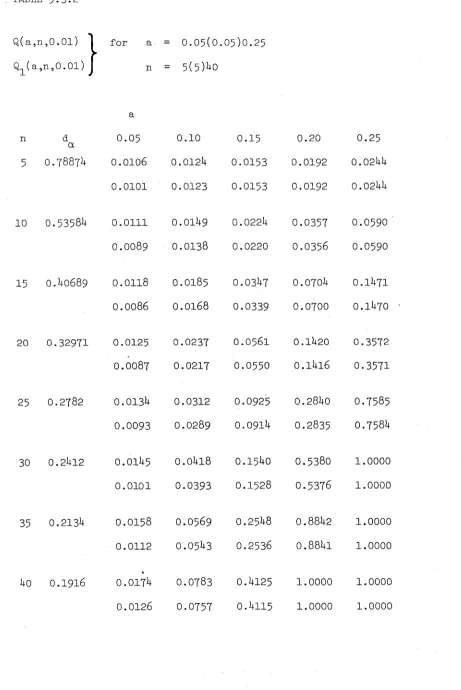
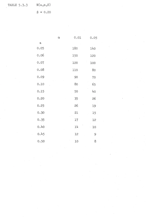
I Appendix to 5.3 165

II Appendix to 5-4 180

III Appendix to 5-5 185

CHAPTER 1

GENERAL INTRODUCTION

In this thesis we discuss a number of problems concerning point processes and Markov processes. There are several themes which emerge

in the course of this study, the most dominant of which are the thinning of point processes and small sample properties, while other problems relate to length biased sampling and time reversal and

several chapters are motivated by applications to neurophysiology. We use a variety of techniques of applied probability, to derive

(joint) interval distributions and second order properties; and of statistical inference, to evaluate the power of certain tests of hypothesis against given alternatives and also in an exercise concerning deficiency.

Much of our discussion lies within the framework of recent accounts of the theory and applications of point processes by Cox and Lewis (1966), Daley and Vere-Jones (1972) and Cox and Isham (1980) and we now summarize those aspects of this theory which are most

pertinent to our discussion. (We note that more esoteric and

generalized presentations of the theory of point processes are also given by Kallenberg (1976) and Matthes, Kerstan and Mecke (1978)).

2.

of the intervals between events or in terms of the number of events that occur in given sets; the latter approach is more useful in the development of the theory of point processes since it can be

generalized to other spaces. We consider the point process II with random non-negative integer-valued (counting) measure N(*) defined on B(R) , the ö-algebra of Borel sets of R; then for each

A G B(R) , N(A) is the random variable for the number of events in A. We denote N((0,t]) by N(t), N((s,t]) by N(s,t] and N(t,t+dt) by dN(t) for infinitesimal dt. We denote the times of occurrence

of events of II relative to a given origin by

{t. ; i £ Z,__ < t < t < 0 < t. < ...}

1 -1 o 1

and the interval sequence of II by {x^ = t^ - t_. ^ , iG Z} ;

t^ and t are known as the backward and forward recurrence times, respectively.

II is said to be stationary in a given sense if some aspect of its probabilistic structure is invariant under translations in time. If its finite dimensional counting distributions have this property, that is, if, for bounded A . Gb(R), A.+t = {a+t;aGA.} , n.=l,2,..

l l l i

and k=l,2,..,

P{N(A +t) = n ; i=l,..,k} (l.l)

is independent of t, then II is completely stationary, while if (l.l) is required to hold only for k=l, II is simply stationary. If the expectation and variance of N(A+t) (all bounded A c b(r)) are independent of t then II is said to be weakly or second order stationary. The interval sequence of II is interval stationary if the joint distribution of {x_^+^; i=l,..,m} does not depend on n .

3.

process is not in general interval stationary, nor is the counting distribution of a stationary interval sequence completely stationary

(Cox and Lewis (1966, . 3 ) , but the stationary counting distribution and stationary interval sequence of a point process can be related by Palm-Khinchin theory (see Daley and Vere-Jones (1972,§7))*

At an intuitive level, to derive stationary counting properties from the stationary interval sequence of a point process involves locating the origin at time t and taking the limit as t becomes infinite; these are referred to as asynchronous or arbitrary time initial conditions (Lawrance (1972,197*0 )• The origin is then located

independently of neighbouring events, so is more likely to fall in a long interval; the probability that it falls in an interval of given length is then proportional to that length and this is known as length biased sampling (McFadden (1962)). Conversely, to obtain

stationary interval properties given the stationary counting properties of a point process we condition on the event

{N(-T ,0]>l) and take the limit as T approaches zero; these are referred to as synchronous or arbitrary event initial conditions.

Now if II is simply stationary its parameter is defined by

A lim

dt-*0

P{dN(t)>l) dt

and its rate is given by

y lim dt-K)

E [ d N ( t )] dt

k.

TT (t) = -A 1 D* p (t) and

o t o (1.2)

\(

t

)

-

Vi(

t

)

=

p

k

(

t

)

*

where D denotes right-hand derivative; these are known as the Palm-Khinchin equations. The generating functions

<f>(z,t) = kf 0 zkpk (t) and 4>o (z,t) = k EQ z^TT^t)

(1.3) therefore satisfy the relationships

D cj)(z,t) = -A(l-z)<|> (z,t) and

t o

•t

cf>(z,t) = 1 - A(l-z) (j) (z,x)dx .

o o

Generalized relationships are also available for joint distributional properties (Lawrance ( 1 9 7 M ) .

Although the finite dimensional distributions are required to specify a point process completely, a lot of the most important and accessible information is contained in the first and second order properties. Let the d.f. of be F ( *) and the d.f. of

(X +..+X ) be F (•), k=2,3,..; if these are absolutely continuous

_L K. K.

we denote their p . d . f . ’s by f (*) and f (•)» respectively.

K.

The first order counting moments for the asynchronous and

synchronous distributions of II are then respectively, the mean-time function

M(t) = E[N(t)] = pt ,

5

oo

H(t) = lim E[N(0 ,t] N(-T,o]>l] = E F1 (t) .

_ K —1 K

When H ( *) is absolutely continuous its density, given by h(t)= E f (t), is known as the 'renewal' density and has the

k=l k

interpretation that h(t)dt is the probability that an event of the synchronous process occurs in (t,t+dt). Provided that there is no long term dependence (e.g. cyclic effects) we have that h(t)-^p as

t - > 00 .

The second order counting properties can be expressed in a number of equivalent ways and require only the assumption that II is weakly stationary. The variance-time curve,

may be represented in the frequency domain by the spectral measure G ( •) satisfying

(Daley (1971)) and if G(•) is absolutely continuous the spectral density g+ (•) satisfies

Now clearly the expected length of an interval of the synchronous V(t) = Var(N(t)) t > 0 ,

V(t) = t2G({0}) + (sin(.^)/|)2G(d0) (1 .4 )

process is

E(x)

pn = Cov(X1 ,X1+n)/Var(X) , n=l,2,.., 1 ’ 1+n

and its Fourier transform, the interval spectrum, is

1 00

f (w) = — (1 + 2 En p cosnoi), 0 < u) < tt .

All of these expressions may he derived, from the count p.g.f. cj)(z,t) given at (1.3):

M ( t ) - ]it - ( 1 »f ) 5

H(t) = 4~<P U , t ) — D*(j>(l,t) anä

az o 2y ^ 2 t

V(t) = — <J>(l,t) + yt - (yt)2 , 9z2

from which G ( •) follows. Also ((1.2) and Cox and Lewis (1966,§U.6))

f*(s) = 1 - ^ ( 1- <f*(o,s)) , (1.6)

Var(X) = p_:L(24>*(o,o) - p"1 ) , (1.7)

pn = TIvSnY7(n! T I . n=l,2,.., and

dz

(1.8)

f+ (w) = -T,Var(X) + • U - 9 )

We now introduce some particular point processes. The Poisson process, which is fundamental to the study of point processes, is an orderly point process such that the probability that an event occurs at any particular time is independent of what happens at all other times. It is therefore referred to as a completely random point process and we denote its instantaneous rate by y(t), t^=R.

Then the number of events on each bounded interval A has Poisson distribution with parameter m(A) y(t)dt, and the distributions

\A

7.

The renewal process is defined as a sequence of i.i.d. intervals \ it is referred to as an ordinary or equilibrium renewal process if it starts in synchronous or asynchronous initial conditions, and as a delayed renewal process otherwise. If the interevent distribution is

absolutely continuous then the p.d.f.'s of the forward recurrence times in these cases are f ( • ) » — (l-F(*)) and f ^ ( •) , respectively, and all subsequent intervals have p.d.f. f (•) . The renewal

function has Laplace transform

H*(s) = F*(s)/(l-f*(s))

and the synchronous count p.g.f. has Laplace transform

4>*(z,s) = (l - f* ( s ) ) /s (1— zf * ( s ) ) .

We may generalize the interval specification of the renewal process further and consider the stationary (first-order) Markov dependent interval sequence of a point process, such that

P{X <x

n X ,i<n} P{X <x X n-1_} ,

e z

8

this in Chapter 2; in particular we follow the account of superposition of point processes given by £inlar (1972), emphasizing situations where a superposed process can be thought of as contaminating a second point process, and we draw together the somewhat scattered literature on the thinning of point processes, which we relate both to contamination and to selective interaction models.

Then in Chapter 3, motivated by a simulation study of contaminated neurophysiological data by Shiavi and Negin (1973), we derive the

distribution of the sample serial correlation coefficients (SCC's) for a finite portion of a renewal process which has been contaminated by particular types of superposition and thinning, noting that certain modifications must be made to the standard (asymptotic) length-biased

sampling results when the population is finite. We obtain the power of a test for the presence of contamination based on the sample SCC’s, which, together with further simulations, leads us to conclude that the SCC's are less sensitive to the presence of contamination than had previously been thought.

In Chapter U we study the class of stochastic point process models known as selective interaction models, where the thinning of a point process (E) is effected by the events of a second point process (i). These have developed in response to the neurophysiological observations of Bishop, Levick and Williams (196U), because of their ability to generate multimodal interevent p.d.f.'s. When I is a renewal process and E is a Poisson process the resulting thinned process lies

9. obtain simplified expressions for the variance-time curve and

interevent p.d.f. for a number of variations of the selection interaction model. We treat the case where E is a renewal process and I is a Poisson process as a generalization of the independent point thinning of Renyi (1956), where the probability that a point is deleted now depends on the length of the interval preceding it. The literature contains many variations of the basic selective interaction model which have been proposed to bring the model "closer to neurophysiological reality"; we categorize there so as to be better able to assess their usefulness in applications.

In Chapter 5 we discuss the inhomogeneous Poisson process for which the rate is alternately a constant and zero on intervals of fixed length,

(which may in fact be interpreted as a variation of the selective interaction model). We give its second order properties and discuss a problem of inference which leads to generalizations of Fisher's classical g-distribution in geometrical probability (for the

distribution of the largest interval on a circle) and in time series analysis (for the distribution of the largest periodogram ordinate). We also make an interesting observation concerning the distribution of the second largest interval on a circle.

In Chapter 6 we show that two Markov chains which have recently been discussed in the literature are time-reversed versions of one

another and give a characterization of the exponential distribution as a converse. These Markov chains may be interpreted as the interval sequences of stationary point processes; the second order properties of one (Gaver and Lewis (1900)) are very much easier to calculate than those of the other (Tavares (1980)).

10. with the unconditional ML estimators of Klotz (1973) and Moore (1979)* Although this is not directly related to point processes, we note that the way the initial state affects our approach to inference is

reminiscent of the way the distribution of the first interval affects the study of renewal processes; and that the way the finiteness of the

sample affects estimation here is reminiscent of the way finiteness

affected the length-biased sampling properties studied in

Chapter 3. In fact we are essentially testing for an unusual effect or outlier at the origin, although we do not pose our problem in that way. For the two-state Markov chain we give a closed form solution for the unconditional ML estimators and use a deficiency criterion to compare conditional and unconditional ML estimation for small samples; we then reconsider the data of Klotz (1972,1973) in the light of these

11.

CHAPTER 2

CONTAMINATION AND OPERATIONS ON POINT PROCESSES

2.1 INTRODUCTION

Much consideration has been given in recent years to the fact that a sample can contain observations which seem odd in comparison to the rest of the data, and that statistical principles should be used to ensure the appropriate analysis. Such observations are known as outliers and Barnett and Lewis (1978) give a comprehensive review of the statistical methodology for identifying, accommodating and rejecting outliers in univariate, multivariate, experimental design, regression and time-series data, pointing out that in highly

structured situations suspicious observations tend to be less

intuitively apparent. They give a formal understanding of an outlier as "an observation which appears to be inconsistent with the remainder of that set of data", or more intuitively, "an observation which is not only extreme, but also extremely extreme". An important aspect of the motivation for this study is the widespread use of the

assumption of normality for modelling the observations, residuals or innovations. It is important then not only to investigate the behaviour of test statistics under the assumptions of the model for different parameter values, but also to discern how robust these statistics are when the assumptions of the model are perturbed somewhat.

12.

and the way it has been modelled. What level of contamination is it possible to detect and what level makes the process unrecognizable? How best should the data be analysed to minimize the effect of contamination? In many respects the Poisson process plays the same role among point processes as the normal distribution does among

univariate distributions. How best can small perturbations of a model be described, and what is the behaviour of test statistics with known distribution for Poisson assumptions (or more general models) under these perturbations? There is no shortage of questions which may be asked, and although no attempt is made to answer them all, they form the general framework for the discussion of the next two chapters.

As we have implied, the traditional understanding of an outlier is not so relevant to point processes as to other types of

data. Except in situations where a point process is highly deterministic, where there is an interval of exceptional length, or perhaps a location of abnormally high intensity, one is not likely to be able to classify a point as odd on the grounds of visual inspection and subjective judgment. Moreover, the first case is uninteresting and the second may be approached by univariate techniques for the interval process.

However, the very complexity of a point process also increases the possibility of a point being "misclassified" and so it is

instructive to look at a number of ways in which a realization can be contaminated. This implies the existence of some source which is separate from the phenomenon being studied and interacts with it causing points to be observed where they should not, or not to be observed where they should, in short, an operation on a point process. There is an established and growing literature pertaining to this which provides a starting point and some technical equipment for

1 3. and in the context of other applications. The operations that are most pertinent in the present context are the superposition of two

or more point processes, the random deletion or translation of points within a process, and the distortion of the time scale. General

discussions relating to operations on point processes are given by- Daley and Vere-Jones (1972 ,§

5

In the remainder of this chapter we review the literature regarding superpositions and random deletions, with emphasis on the situations where they are relevant to the study of contamination, although there are many interesting results which are not directly related but which we mention for the sake of completeness. This is particularly so in the case of deletions, for which the literature is considerably more scattered than for superpositions. Our purpose for doing this is to provide a broader context for Chapter 3, where we will consider the sensitivity of the sample serial correlation

coefficients to contamination by the superposition of a "false addition" or by thinning; and to introduce the ’interval thinning’ of point

processes, aspects of which we discuss in more detail in Chapter h.

Although the work of Chapter 3 indicates that the presence of false additions or false deletions has only a small effect on the distribution of the sample serial correlogram, it is well-known that the serial correlation coefficients are more sensitive to sampling

fluctuations than the second order counting statistics (Cox(l963), Cox and Lewis(1966)). In fact problems will often be involved in discriminating between different models on the basis of any of the

second order properties. Models based on exponential autoregressive- moving average sequences have been developed by Lawrance and Lewis (i960)

Chapter 6 in a quite different context.

Perhaps the most useful conclusion we may draw from this

chapter is that, although the subject of outliers in and contamination of point processes has received very little attention in its own right, some aspects of recent studies into operations on point processes

15.

2.2 SUPERPOSITION

In this section we discuss the superposition of point processes in general, with particular emphasis on known results that are

relevant to the study of contamination by "false additions". The observed process II is the superposition of the n processes

II , i=l,..,n , and we assume that the points of the component processes cannot be distinguished. We are most interested in the case n=2,

where IT^ is the process we wish to study and II , the contaminating process, is a Poisson process independent of II . In particular cases it may be desirable to consider a more complex mechanism for generating the false additions, which in fact we do in Chapter 3 where the process of "FB's" is dependent on II .

Now a comprehensive review of the theory of superposed point processes is given by Cinlar (1972), while Cox and Isham (1980) also give an overview of the subject. These discussions fall into three broad categories, which we consider in turn.

The first type of result we consider is the Poisson limit

theorem, which dates back to Palm (l9*+3) and Cox and Smith (1953, 195*0. Khinchin (i960) proved sufficient conditions for the superposition of

stationary orderly independent point processes to approach the Poisson process for large n , while the most general form of the result is given by Franken (1963) and Grigelionis (1963). It is assumed that the component processes are independent, although they are not

16.

component process can dominate the rest. If the components are stationary or clustered processes then II approaches the

homogeneous Poisson process or the clustered Poisson process, respectively, and multivariate generalizations also hold. These results are important as they justify the -widespread use of the Poisson process in many applications, such as the studies of

telephone traffic, nerve processes, computer failures, radioactive decay, light, etc.

A second type of result, which deals mainly with the

characterization of the Poisson process among renewal processes in terms of the type of component and resultant processes which are possible under specified conditions, has undergone some important developments since Jinlar (1972). We recall that the superposition of independent Poisson processes is Poisson, and first consider the case where n=2 and II and II are independent. McFadden and

Weissblum (1963) give the result that, if II and II are stationary renewal processes for which the interval distribution has finite

variance and II is a stationary renewal process, then 11^, II2 and II are Poisson processes. This result was improved by Mecke (1969), who showed that it was not necessary to assume that the interval distributions of II and II^ had finite variance, while Chung (see £inlar) and Samuels (197*0 showed that it also holds when II and n2 are ordinary renewal processes. McFadden and Weissblum's result was generalized by Ambartzumian (1967) to the case in which the interval process of II is a finite-order Markov chain, and by

IT. process. That it is not also necessary for II to be a Poisson

process was demonstrated by Daley (1973a), who showed that the

superposition of a Poisson process with parameter X and an alternating renewal process with exponential interval distributions with parameters P and A 2/y , was a (non-Poisson) renewal process. Daley (1973b) illustrated this further by giving conditions under which the super­ position of a Poisson process with a process whose points are the jump epochs of a stationary irreducible continuous-time Markov chain is a renewal process.

Relaxing the assumption that n=2, it follows that, if the

superposition of a finite number of independent identically distributed renewal processes is also a renewal process, then all processes are Poisson (Stornier (1969)). Ito (1980) generalized this by proving that if the superposition of a finite number of independent identically distributed general point processes is a renewal process for which the interval distribution has density f(•) which is finite at the origin, then all processes are Poisson. Results have also been obtained when the assumption that 11^ and 11^ are independent is relaxed, and are discussed in £inlar (1972).

These results are pertinent to the study of contamination since we have assumed that II is a Poisson process. If we observe that the interval structure of II is no more complex than

finite-order Markov and that II is not a Poisson process, then we can be assured that 11^ is not a renewal process. If on the other hand we observe that II is a Poisson process, this implies that 11^ must also be a Poisson process, so that it is impossible to separate the process being studied from the effect of contamination.

Approaches to statistical inference for superposed processes are discussed by Cox and Lewis (I966,ch8) and Lewis (1972 b), and draw heavily on Poisson limit theorems and ad hoc techniques related

18. independent point processes are inherited by their superposition and the count analysis of superposition processes is generally much more

straightforward then their interval analysis (Cox (1963)). Consequently the interval analysis may often be more useful in yielding relevant

information concerning the number and nature of the superposed processes. A rigourous derivation of the joint distribution of any finite number of

contiguous intervals of the superposition of any finite number of independent point processes is given by Lawrance (1973), which in principle yields all the serial correlation coefficients and the

interval spectrum. His results gather a somewhat scattered literature in which interevent p.d.f.’s and serial correlation coefficients have been calculated for a number of special cases.

For the stationary (independent) component processes II , i=l,..,n, we denote the intensity parameter by X_^, the survivor function of the interevent distribution by F^(•) and the joint survivor function for a pair of contiguous intervals by F.(.,.). Lawrance (1973) shows that the corresponding properties of II

(dropping the subscripts) are given by

X = X_ + . . + X

1 n (2.2.1)

F(t)= i h f Fi(t) jPi j F.(x)dx , and_J (2 .2 .2 )

F ( t >u) = iL. x Fi ( t >u)j?i L F ._J (x ) dx (2.2.3) t+u

which, in the case that the components are identically distributed (substituting the subscript 'o' for the components) reduce to X =nX ,

19.

F(t) = F (t)(A

° 0 it o

(2.2.U)

r°°

F(t ,u) = F (t,u)(A

o o

t+u

F (x ) dx)n

o

Equation (2.2.1) was originally given by Khinchin (i9 6 0); (2.2.2,3) were derived heuristically by ten Hoopen and Reuver (1 9 6 6) for the case n=2, while (2.2.1+) is a well-known result dating back to Cox and Smith (195*0» which has been used by Barnett (1970) to

arbitrary interval distribution, and by Downton (1 9 7 2) when the intervals of the component renewal processes are the sum of a fixed number of exponential random variables.

From (2.2.2,3) it is possible to derive pi, the first serial correlation coefficient of II , for which explicit expressions were given by ten Hoopen and Reuver (1 9 6 6) when IT is a Poisson process and n2 is a general point process. Lawrance also gave an explicit expression for P2, the second serial correlation coefficient, when n is Poisson and II is renewal, together with tables for Pi and P2 for various combinations of gamma renewal processes. These indicate (among other things) that when II is Poisson and 11^ a gamma renewal process with integral index a , that Pi is small and increases with a and that P2 is very small (results which complement the sample properties we will derive in Chapter 3).

Barnett (1970) presented the serial correlation coefficients obtained from a simulation study of the case n=8 when the components are identically distributed renewal processes with delayed gamma interval distribution. This has a distinctive dependence on n when the delay is large compared to the mean of the gamma distribution, showing approximate F(•) when the components are renewal processes with

2 0.

may "be slow. Enns (1970) also studied the serial correlation coefficients for the superposition of n independent renewal processes, showing that when the renewal density has increasing

2

hazard rate then Pi > -l/2n . Proudfoot and Lampard (1973) gave the serial correlation coefficients for the point process obtained by retaining every k"^ event of the superposition of n independently phased identically distributed deterministic point processes.

Finally, Ambartzumian (1965,1969) discussed two problems which are more directly related to the present context. Following him we take A=l. His first problem is, given a realization of the

superposition of an unknown number of identically distributed renewal processes, to deduce n , the number of component processes and

F (•), the renewal interval survivor function. He gave n as a function of m (0) and m ^ O ) , where (for i=l,2)

m.(t) = T T E[N(s,s+t]|N(0,s]>i]

1 dt

-s-KD

and N(*) is the counting measure for II . By expressing these as a function of the derivative of t h e ’renewal1 function at zero, which may then be eliminated, it follows that

n = (l-m1 (0))/(l-m1 (0)-m1 (0)2+m1 (0)m2 (0)) .

F (•) may then be derived from the empirical survivor function of o

II by the inverse relationship to (2.2.U)

F (t)

o F ( t ) ( F(x)dx)n

21.

His second problem is, given a realization of the superposition

of a Poisson process and a renewal process, to deduce A* , the

Poisson rate and F( • ) , the renewal interval survivor function.

Using the above techniques it transpires that Xi is given by the

root on (0,l) of the quadratic equation

(m1 ( 0 ) -l)A^+ m 1 (0)(l-m2 (0)) Ai+ m 1 (0)(m2 (0)-m1 (0)) = 0

and that the inverse relation for F (•) is

o

F (t)

o (F(t) - A,

F(x)dx)

' t

(2.2.5)

However, he also gave a more useful, although not necessarily

optimal, method of inferring Ai , which is based on relating the

interval properties of II and ITi (the remaining points in II

after independent thinning as discussed in the next section) from which

a relationship is deduced between and some of the interval moments

of II . If we denote by m 2 , m^ and c the second the third

interval moments of II and the covariance between adjacent intervals

of II , respectively, then

X i

equation

(3m2 - 2 m )A* + 2(6c-6m2+m +6)

X 1 -

and F (•) can be derived from (2.2.5). Plainly the calculations

o

involved here are much more stable than those of the previous method,

and (2.2.6) has a useful role in the detection of contamination

22.

2.3 DELETION

We now consider the situation where some points of a point

process are deleted, resulting in a thinned point process. An overview of this subject is given by Cox and Isham (1980). In the same way that we can define point processes in terms of either their interval or counting properties, so we can also specify the thinning operation in relation to intervals or points. Firstly, consider the situation where points are deleted because they fall into particular intervals. There is an extensive literature on counter models (Cox and Isham

(1980,pl01)) which describes the behaviour of, for example, a device which counts radioactive particles and is paralysed every time a

particle registers. A particle arriving while the counter is paralysed will not be counted and so is deleted from the incident stream; thus the interval thinning operation is dependent on the original process. If on the other hand points are deleted because they lie in an

interval of an independent process, we may treat the thinned process as the response process of some version of the selective interaction model; we discuss both this and counter models further in Chapter U, together with a model which is developed from the selective

interaction models, where the probability that a point is deleted is a function of the length of the interval preceding it.

2 3. extensive literature which is in part traced by Szasz (1976) from Renyi’s (1956) classic paper to the publication of his selected works, while Serfozo (1977) places his very general results in the

context of the mainstream of this work and Galambos and Kotz (1978) also give bibliographical notes (and relate the independent thinning of renewal processes to the broader context of damage models).

There is particular emphasis on Poisson limit theorems of a similar flavour to the theorems for the superposition of point processes referred to in the previous section.

We consider the univariate point process II with counting measure N ( •) , for which we may represent the realization

T = {t.; i £ Z} (where Z is the integers) by

dN(t) dt

Z

i G Z 6(t-t^)

where 6(*) is the Dirac delta function. When II is a renewal process we will denote its p.d.f. by f(•) , with expectation y . We define 11^ , the thinned version of II with counting measure N^( * ^ 9 associating a binary random variable x^ with t^ for each i G Z. If x. is zero then t. is deleted from the

l l

realization, while if x^ is one is retained. We may represent T , the realization of II corresponding to T, by

d d

dN (t) y

= is h 5(t-V

It is usually supposed that points are deleted in blocks, the number of points in which is a specified discrete random variable, and so we define

2h.

The expected number of deleted points between retained points is then <x-l

01 = Ii nq_^ . When a becomes large the points of II are very sparsely scattered and so we may rescale it by a factor of a-1 to obtain n_^ , which will then have the same intensity as II . We

denote the counting measure of II by N (•), and the deleted-rescaled

r r

realization corresponding to T by T^, which has the representation

dN (t) r

dt £ X-

6(t-t./a) •

iez

Most attention has been paid to the important case of stationary independent thinning, where the {y±) are independent identically distributed random variables and the block length has geometric distribution q^ = qpR 1 , with 0<p<l, q=l-p and a=q-1 . The earliest results are given by Renyi (1956) when II is a renewal prooess, with interevent p.d.f. f (•) having expectation y . Then

II is also a renewal process with interval p.d.f. given by r

fr (t) = q n? 1 pn_1 fn (t/q) , n*

where f (•) is the n-fold convolution of f (•) • Renyi showed that II has the same distribution as n_^ if and only if it is a Poisson process (that is, the Poisson process is the only renewal process invariant under the deletion-rescaling operation); and that if y is finite then the limit of II as q approaches zero is the homogeneous Poisson process process with parameter y ^ . He also gives an example to show that it is possible to obtain a Poisson limit when y is infinite by using a modified thinning­

rescaling procedure. Kovalenko (1965) and Gnedenko and Fraier (1969) obtain an expression for the possible limit distributions which may result from the usual thinning-rescaling procedure when y is infinite, and demonstrate the existence of renewal distributions which lead to these limits (see alternatively Gnedenko and Kovalenko

25.

Nawrotzki (1962) generalized Renyi’s limit theorem by shoving that if II is a general stationary point process then II has a unique limit as q approaches zero which belongs to the class of doubly stochastic Poisson processes. Belyaev (1963) proved that a condition involving the law of large numbers was sufficient for this limit to be a homogeneous Poisson process, which Westcott (1976) improved and simplified, also proving its necessity. For higher dimensional Euclidean spaces extensions are given by Goldman (1967) and Tulya-Muhika (1971), while Kallenberg (1973, 1975), drawing on results for compound point processes, proved the doubly stochastic Poisson process limit theorem for point processes on topological spaces and derived as a corollary the result of Mecke (1968) that a point process is a doubly stochastic Poisson process if and only if for each p£(0,l] it is the independently thinned version of some point process.

It would appear that all required results concerning limit theorems for independent thinning of stationary point processes are contained in Kallenberg (1975) and Westcott (1976).

Perhaps the earliest work on dependent thinnings (i.e. the case where the block length does not have geometric distribution) is by Polyak (1966), who derived bounds for the counting distribution of renewal processes thinned in a quite general way. Dietz (1968) considered the interval distribution of I I w h e n II is a renewal

d

process and the form a first-order two-state Markov chain, n_2

so that q^ = (l-a) (l-(3)a , 0 < a,8 < 1. As an aside we note that he demonstrated the ability of this scheme to produce multimodal p.d.f.’s , which is not at all surprising as the thinning of an

26. of first order properties. We note that it is possible to write down the likelihood for thinned renewal processes, and so the problem of estimating the thinning distribution and renewal interval distribution can be carried out on a formal basis, unlike the complementary case for the superposition of renewal processes as discussed by Ambartzumian

(1965,1969)(see the previous section). Isham (1980) extended Dietz's work in considering the counting properties and limiting interval

distribution for the thinning of general point processes when the are first-and higher-order Markov chains, and in particular, found that as a approached infinity the interval distribution of the

limiting thinned-rescaled process was a mixture of a point mass at the origin and an absolutely continuous exponential component. That other limiting distributions are possible for different block length

distributions is evident from Räde (1972b), who showed that 11^ tended towards the deterministic point process for large a for any renewal

interval distribution f(•) when the {q^} were Poisson, compound Poisson or binomial probabilities,while a limiting gamma process was also possible if the {q^} were negative binomial. These are somewhat surprising results and appear to be related to the small coefficient of variation of the number of points in a block as the mean becomes large. Räde also discussed invariance under thinning and rescaling. Further results for the dependent thinning of renewal processes were given in a series of papers by Szantai (1971a,b) and Mogyorodi

(1969,1971,1972,1973), who showed (i) that the limiting interval

distribution after repeated thinning and rescaling belong to the class of limiting distributions for supercritical Galton-Watson branching processes. He extended this (II) to the case where the average

interval length of IT is infinite, and obtained conditions for

2 7.

mechanism, the most interesting of which is that of VI where the probability of deletion of a point also depends on its time of occurrence. Writing q(t) = P{x^=l| t_^=t}, Mogyorodi investigated the counting distribution of the thinned process and derived a Poisson limit theorem. This is also the formulation used by

Brillinger (1979) to study the major events in China's seismic history, the record of which is almost certainly deficient as documents from the more distant past have been lost. Brillinger gives asymptotically unbiased estimators for the required first and second order properties, both when q(t) is known and when it is specified by a finite

dimensional parameter. Some of Mogyorodi's results have been extended by Szynal (1976) to sequences of independent but not necessarily

identically distributed random variables. There is further work on limit theorems for dependent thinning of multivariate point processes leading to Poisson limits by Tomko (197^0 and of point processes

on topological spaces by Jagers and Lindvall (197^) and Serfozo (1977), whose paper is set in the most general context, containing extensions to the thinning of random measures, and so subsumes most other work on thinnings.

28.

29.

CHAPTER 3

CONTAMINATED RENEWAL PROCESSES AND THE SERIAL CORRELOGRAM.

3.1 INTRODUCTION

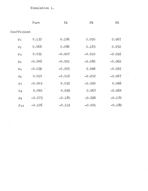
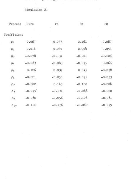
In this chapter we study the effect of contamination on the serial correlation coefficients (SCO’s) of a finite portion of a renewal process. We will consider three types of contamination:

(i) (FA) the false addition of one point uniformly distributed on the realization, so that the probability that it falls into a given interval is proportional to the length of that interval,

(ii) (FB) the false addition of one point uniformly distributed on a randomly chosen interval, and

(iii) (FD) the false deletion of one randomly chosen point.

We will refer to the uncontaminated process as the pure process, and to those contaminated as above as the FA, FB and FD processes,

respectively.

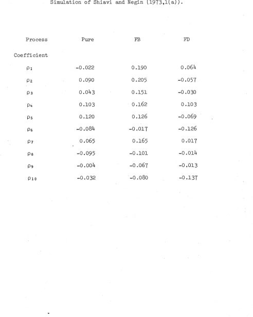
Shiavi and Negin (1973) considered the effect of such contamination in the context of neurophysiology, where due to

automated data recording techniques it is possible to observe a spike arising from some source other than the neuron under consideration, or to fail to observe a real spike, perhaps by setting too high a threshold. They simulated (by computer) a renewal process and first- and second- order Markov processes with a specified number (100, 200 and 500) of normally distributed intervals with coefficient of

30. with FB's and FD's . They found that a systematic positive bias

resulted from an F B , which was significant for the first few SCO’s; a corresponding negative bias resulted from an FD, although it did not in general reach the same level of significance.

This raises the question of whether the behaviour of the

theoretical serial correlogram (SCG) and the statistical

distribution of the sample SCG are similar to that of the simulations. Ten Hoopen (1975,1977) studied the theoretical SCO's of contaminated renewal and first-order Markov processes, but unfortunately his results are inapplicable to the present study of renewal processes for three reasons. Firstly, he assumed that Shiavi and Negin had used FA's in their simulations, whereas in fact they had used FB's

(personal communication from Dr R. Shiavi), although they did not state this clearly in their paper. For this reason we perform our analysis for both FA's and FB's, noting that the FB is not a natural type of contamination. Secondly, in his treatment of FA's, ten Hoopen compensated for the fact that an FA is more likely to

fall in a large interval, but for a finite number of intervals one must also compensate for the fact that it is correspondingly less

likely to fall in a small interval. This leads to awkward contradictions and will be further discussed in 3.2. Thirdly, the FA interval

sequence is not stationary, and so there is no formal definition of the SCC's, although the ad hoc definition ten Hoopen adopts does have merit in characterizing the expected behaviour of the sample SCG. These factors combine to yield expressions for the theoretical SCC's

for samples of size N which are in fact in error by an amount which is 0(N ■*■) , and since the expectation of the SCC's for a renewal process is also 0(N ^), his results are inapplicable in that context.

31.

the expressions his method leads to for p , the serial

correlation coefficient of order n for contamination of type i, where the N intervals of a renewal process are normally distributed

2

with mean y and variance O :

P lb

i y 2 - 3q2 K 6o2-8p2

+ o(N 1 ),

p nb

-1 (2n+l) y2 + (n-1) a 2 +04 /y2 , -2

N(N-n-l) --- ---- --- + ° (N n=2,3,...,

P nd

2n - 1

N(N-n-l) + o(N 2 ), a4

n-l,2,

These may be compared with equations (3.H.1-3).

However, in this chapter we deal with the statistical distribution of the sample SCG. We test the null hypothesis that the interval

sequence comes from the realization of a renewal process against the alternative hypotheses that the renewal process is contaminated by one FA, FB or F D , and derive the distribution of the SCG under these alternatives, hence deducing the power of the tests, that is, the probability of correctly diagnosing contamination. (in so doing the question of stationarity does not arise).

In 3.2 we evaluate the interval moments for a length-biased sample from a finite number of intervals of a renewal process and in 3-3 we establish the notation to be used in the ensuing sections. The main results are given in 3.^ and an outline of how they were derived

follows in 3.5- In 3.6 a simulation study is presented as a comparison to that of Shiavi and Negin, and 3.7 comprises a discussion and

32.

3.2 LENGTH-BIASED SAMPLING FROM A FINITE POPULATION

As ten Hoopen observed, the occurrence of an FA has a length- biased sampling effect, that is, the probability that an FA falls

in an interval of given length is proportional to the length of that

interval. Results for this are well-known when the sample is taken

from an infinite population ( McFadden(1962),Cox & Lewis(1966, § i .2)). For

a renewal process with intervals {X^;i=0,1,..} with p.d.f. f (.),

o

mean y, variance o and higher order moments y ,r=2,3,.., a

length-r

bias sampled interval, X, has p.d.f. f^.(x) = >

expectation y2/yi, variance (yyä-yf)/y12 and higher order moments

X

y = y ,/y, r=2,3,.., while the properties of those intervals not

r r+1

sampled remain unaltered.

However, when a finite sequence of N intervals of a renewal

process {X. ;i=l,.. ,N} is "sampled" by an FA falling in X^

these results require modification. (Otherwise we would have that the

expected length of the record was that of N-l ordinary intervals plus one length-bias sampled interval, which is equal to Ny+Q2/y; while it is, of course, unaltered by the addition of an FA, and so

equals N y . ) We define Y. = X for i = -m+l,..,N-m. Given

l m+i

that the length of the realization is T , the probability that

the ith interval is selected is simply p^ = X /T^, i=l,..,N, and

so we may write the expectation of as

N 2

E(Y0 ) =.|1E(X.p.) = N E (q/Tjj) , and

1 H

E(Yi ) = iüT i=iE(xi(l-pi )) = n e (x1X2/t n) >

where Y^ is taken as representative of all intervals not equal to

Yq . Expressions for higher order moments may be derived similarly.

n r^

3 3.

p o s i t i v e i n t e g e r n < N a n d r n , . . , r > 0 ( w i t h r = . X _ , r . - l ) .

l n i = l i

We may d e r i v e a f i r s t o r d e r a p p r o x i m a t i o n f o r t h i s u s i n g t h e r e l a t i o n

f o r moments o f a q u o t i e n t

w Ün ~ E( u ) ( C o v ( u , v ) V a r ( v ) x

V ~ E ( v ) U - E ( u ) E ( v ) e ( v ) 2 j

E ( u ) E ( u v ) , E ( u ) E ( v )

E ( v) E ( v ) 2

E(-w h i c h i s d e r i v e d u s i n g t h e b i n o m i a l e x p a n s i o n ( s e e K e n d a l l a n d S t u a r t ,

1 9 7 6 , § 4 8 . 3 ) , a n d r e q u i r e s t h a t v i s n o n - n e g a t i v e . T h e n , s e t t i n g r .

n - q

u = . TI X. a n d v=T , s o t h a t i = l i

we o b t a i n

E ( u ) = H y , E ( v ) = Np ,

1 i

E( uv) = ( l i t ) £ ( p -,/p ) + ( N - n ) p ( n p ) ,

1 i 1 i i 1 r i

E ( v ) = N p2 + N(N-1 )y 1 ,

n r

N E ( II X. 1 / ^ ) = ( n yr / y ) [ l + ( y 2- p 2 - y X ( y r +1" W r ) / P r ) /Np2 ]

1 1 r i 1 r i i i

+ o(N- 1

Hence

V>2 b3 y2 q

e(y1 ) x y - ^ (vi2 - y2 ) ,

2 U3 "I V i 2 h 3

) ,

E(YqY1 ) = E(Y2 ) * y2 - ^ j ( y 3- y y 2 ) , and

3b.

T T • y2 y3 lVl\2 A

We recognise — * , — --\ — ) and [— ---t-) as the mean and

y y y y p

variance of YQ and E(Y3) - E(Yq)E(Y2), respectively, in the case of an infinite population, so that it is clear that the coefficient of N 1 is always negative. It is also clear that these results

converge to those for an infinite population as N^°°.

For the gamma interval density, f(x) = x e /T(a),

approximation is unnecessary. We are able to obtain exact expressions for the moments since (X^/T^,..,X^/T ) has a Dirichlet distribution (see, e.g. Wilks (1962)) and is independent of T^t , which has gamma distribution with parameter Na. Hence

E(n x.1/1^ ) = E[(n(x /t ) P tW

i=l 1

n

= J (T(a+r )/r(a))/(aN+r) . (3.2.1)

This generates the following expressions which are used to derive the results of the following sections :

E(Y ) = Na(a+l)/(aN+l),

E(Y ) = Na2/(aN+l),

E(Y2) = Na(a+1)(a+2)/(aN+2),

E(Y Y ) = E(Y2 ) = Na2(a+l)/(aN+2),

E(YiY2) = Na3/(aN+2),

E(Yq) = Na(a+l)(a+2)(a+3)(a+l+)/(aN+i+),

E(Y3Y1 ) = E(Y^) = Na2(a+l)(a+2)(a+3)/(aN+4),

E(Y2Y2) = E(Y Y 3) = Na2(a+l)2(a+2)/(aN+U),

35

.

E(Y0Yl V = E(YiY2) = Na3(a+l)(a+2)/(aN+l+) ,

E(Y0Y1Y2 ) = = Na3(a+l)2/(aN+l+) ,

E(YqY1Y2Y3) = E(Y2Y2Y3) = NaU(a+l)/(aN+4),

36.

3.3 NOTATION

Let {X_^; i=l,..,N} Le the sequence of intervals of the set of points T={T.; T =0,T.=T. +X. , i=l,..,N}, where N is a constant

l 0 l l - l l

positive integer. We assume that the intervals come from a renewal process with gamma interval density f(x) = x e /T(a), forming a stationary sequence. We prefer the gamma density to the normal (used Ly Shiavi and Negin (1973)) since it is desirable to eliminate the

possibility of negative intervals in theoretical work., while there is no practical chance of simulating a negative interval when the coefficient of variation is 0.2. Moreover, we recall that as a increases the gamma distribution approaches normality and that for a >25 the coefficient of variation is less than 0.2. We also note that Shiavi and Negin (1975) preferred to use the gamma density in their application.

By an FA we mean the addition to T of the point T, uniformly distributed on [0,T..] . We can assume that T _ < T < T , that is,

’ N m-1 m ’ ’

th

T falls in the m interval for some m=l,..,N, since with

probability one T f T^ , for i = 0,1,..,N . This leads to the interval sequence {lh}, say, defined by

(i = 1,..,m-1) (i = m)

(i = m+1)

(i = m+2,..,N+1) .

37.

1

—

1

X

with probability

1 a h/t n

u T with probability

_V

_tm

_and

r

i-(

with probability

x i/t n

l T-h

then E(UX ) = E(X1 ) - %E(X^/Tn ) and E(U2 ) = E(X2 ) - E U ^ / T ^ .

2 -1

But we know from the previous section that E(X^/T^)=E(X )('a+l)/(oi+N ) and E(X1X2/TN )=E(X1 )a/(a+N_:i) i %E(X^/Tn ) (except for a=l).

By an FB we mean the addition to T of the point T ’ , uniformly distributed on (T _ ,T ) , where prob(m=i)=N ^ for

m-1 m

i=l,..,N. This leads to the interval sequence {V^}, defined by

X. 1 (i 1— 1 S 1— 1 II

T ' - T „ (i = m) m-i

T - T' U = m+l) m

X

H

- _{1 H} (i = m+2,..,N+1)

Again, {V.} is not stationary since E(V^) = (l-%N ^)E(X^)/

(1-tC1 )

By an FD we mean the deletion from T of the point T , where prob(m=i)=(N-l) ^ for i=l,..,N-l. This leads to the interval

{VA } defined by

f

A

L

The sample serial correlogram (see, e.g. §45-32 of Kendall and Stuart (1976)) for {X.;i=l,..,N} is given by r =a /b ,

1 n n n

38.

, M M M

a = M .E X. X. - M .E_ X. .E_ X.

n i=l l l+n i=l l i=l i+n

M M

-1 2 -2 11 2

b = M .EX. - M (.E X . ) , and

n i=l i xi=l i 5

M = N-n.

Analogous expressions hold for the contaminated processes. The

denominator b^ is not standard, but as Kendall and Stuart point out

at equation (^5-53), it is a sufficiently good approximation when N

is not too small. To avoid end effects in calculating the SCC of

lag n we will further assume that the random index m is

restricted to m£{n+l,..,M-l}. So far as we can tell these

approximations introduce errors into the moments of r that are at

n