Performance and stability analysis of an AC variable speed drive

UNIVERSITY OF SOUTHERN QUEENSLAND

Faculty of Engineering and Surveying

Performance and Stability Analysis of an AC

Variable Speed Drive

A dissertation submitted by

Andrew Stewart Rae

in fulfilment of the requirements of

Courses ENG4111 & ENG4112 Research Project

towards the degree of

Bachelor of Engineering (Electrical & Electronic)

Abstract

In this dissertation an experimental, speed sensorless, AC variable speed drive is developed from works presented by previous researchers and the performance and stability of the drive is analysed. The experimental drive consists of a simple control algorithm that can be implemented on low cost systems and provides a performance that is superior to standard constant V/f drives.

There has been a great deal of research into AC variable speed drives and many different speed control schemes have been developed which range in complexity, performance and cost. Open-loop scalar control techniques are generally the least expensive to implement as no motor speed sensor is required. These techniques are likely to prevail in applications where instantaneous speed and position control of induction motors is not critical. Such applications may include pumps, fans and conveyors.

UNIVERSITY OF SOUTHERN QUEENSLAND

Faculty of Engineering and Surveying

ENG4111 & ENG4112 Research Project

Limitations of Use

The Council of the University of Southern Queensland, its Faculty of Engineering and Surveying, and the staff of the University of Southern Queensland, do not accept any responsibility for the truth, accuracy or completeness of material contained within or associated with this dissertation.

Persons using all or any part of this material do so at their own risk, and not at the risk of the Council of the University of Southern Queensland, its Faculty of Engineering and Surveying or the staff of the University of Southern Queensland.

This dissertation reports an educational exercise and has no purpose or validity beyond this exercise. The sole purpose of the course pair entitled “Research Project” is to contribute to the overall education within the student’s chosen degree program. This document, the associated hardware, software, drawings, and other material set out in the associated appendices should not be used for any other purpose: if they are so used, it is the entirely at the risk of the user.

Professor R Smith Dean

Certification

I certify that the ideas, designs and experimental wok, results, analyses and conclusions set out in this dissertation are entirely my own effort, except where otherwise indicated and acknowledged.

I further certify that the work is original and has not been previously submitted for assessment in any other course or institution, except where specifically stated.

Name: Andrew Rae Student No: 0031210726

Signature

Acknowledgments

Table of Contents

TUTable of ContentsUT...i

TUList of FiguresUT...ii

TUList of TablesUT... iii

TUNomenclatureUT...iv

TU1.UT TUIntroductionUT...1

TU1.1UT TUBackgroundUT...1

TU1.2UT TUAim and Objectives of the ProjectUT...3

TU1.3UT TUOutline of DissertationUT...4

TU2.UT TUPrinciples of Induction MotorsUT...5

TU2.1UT TUConstructionUT...5

TU2.2UT TUOperationUT...6

TU2.3UT TUDynamic EquationsUT...7

TU3.UT TU2 Phase Model of Induction MotorsUT...11

TU3.1UT TUReference FramesUT...11

TU3.2UT TU3 to 2 Phase TransformationUT...12

TU3.3UT TUDevelopment of 2 Phase ModelUT...16

TU4.UT TUImplementation of IM Model in SimulinkUPU ® UTP...20

TU4.1UT TUIM SimulinkUPU ® UPU ModelUT...20

TU5.UT TUVerification of IM ModelUT...25

TU5.1UT TUTesting and Model VerificationUT...25

TU5.2UT TUParameter Testing of IMUT...26

TU5.3UT TUVerification Testing of IMUT...31

TU5.4UT TUVerification of ModelUT...34

TU6.UT TUPrinciples of AC VSDUT...39

TU6.1UT TUAC VSDsUT...39

TU6.2UT TUDC-Link VSD ConstructionUT...39

TU6.3UT TUDC-Link VSD OperationUT...40

TU6.4UT TUConstant V/f ControlUT...42

TU6.5UT TUStator Resistance Voltage Drop CompensationUT...43

TU6.6UT TUSlip CompensationUT...43

TU7.UT TUExperimental VSDUT...45

TU7.1UT TUExperimental VSD ControlUT...45

TU7.2UT TUExperimental VSD Control EquationsUT...45

TU8.UT TUImplementation of VSD Model in SimulinkUPU ® UTP...51

TU8.1UT TUVSD ModelsUT...51

TU9.UT TUStability and Performance Analysis of DriveUT...54

TU9.1UT TUStability and Performance Analysis MethodologyUT...54

TU9.2UT TULinear Stability AnalysisUT...55

TU9.3UT TUSmall Signal Displacement Stability AnalysisUT...61

TU9.4UT TUPerformance AnalysisUT...68

TU9.5UT TUPerformance and Stability EvaluationUT...76

TU10.UT TUConclusionUT...78

TU10.1UT TUAchievement of Project ObjectivesUT...78

TU10.2UT TUProject OutcomesUT...79

TU10.3UT TUFurther WorkUT...79

TUBibliographyUT...81

TUAppendix A – Project SpecificationUT...82

TUAppendix B – Power Measurement for TestingUT...83

TUAppendix C – Stability AnalysisUT...85

TUDerivation of Closed Loop System EquationsUT...85

TUDerivation of Small Signal Closed Loop System EquationsUT...88

TUAppendix D – MatlabUPU ® UPU Function for Linear Stability AnalysisUT...96

TUAppendix E – MatlabUPU ® UPU Function for Small Signal Stability AnalysisUT...98

TUAppendix F – Complete Experimental DriveUT...101

List of Figures

TUFigure 2.1 Induction Motor ConstructionUT...6

TUFigure 2.2 Wye Induction Motor Equivalent CircuitUT...7

TUFigure 2.3 Winding DistributionUT...9

TUFigure 3.1 Reference VectorsUT...12

TUFigure 3.2 IM Field OrientationUT...13

TUFigure 4.1 Stator Direct Phase Sub-Function BlockUT...21

TUFigure 4.2 Electromagnetic Torque Sub-Function BlockUT...21

TUFigure 4.3 Stator Voltage 3-2 Transformation Sub-Function BlockUT...22

TUFigure 4.4 Stator Current 2-3 Transformation Sub-Function BlockUT...22

TUFigure 4.5 IM SimulinkUPU ® UPU ModelUT...24

TUFigure 5.1 IM Test BedUT...26

TUFigure 5.2 Inertia Test - RecordingsUT...30

TUFigure 5.3 DOL Start Test – Stator Line CurrentUT...32

TUFigure 5.4 Sudden Removal of Load Test – Speed Calculated From Armature VoltageUT...33

TUFigure 5.5 Sudden Removal of Load Test - Stator CurrentUT...33

TUFigure 5.6 Sudden Application of Load Test – Stator CurrentUT...34

TUFigure 5.7 DOL Start - Simulated and Recorded Stator CurrentUT...36

TUFigure 5.8 Sudden Removal of Load - Recorded and Simulated Stator CurrentUT...37

UTFigure 5.9 Sudden Application of Load - Recorded and Simulated Stator CurrentsT38U TUFigure 6.1 DC-Link Conversion VSDUT...40

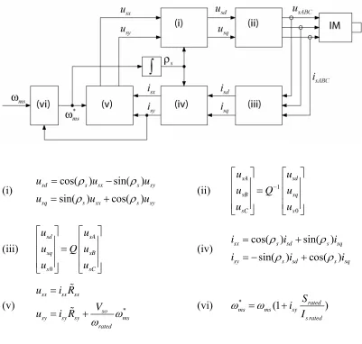
TUFigure 7.1 Experimental VSD Block DiagramUT...50

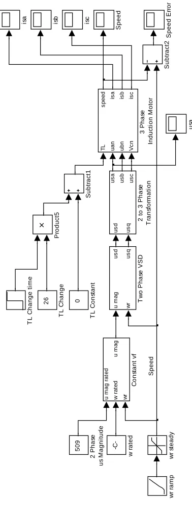
TUFigure 8.1 Constant V/f SimulinkUPU ® UPU ModelUT...52

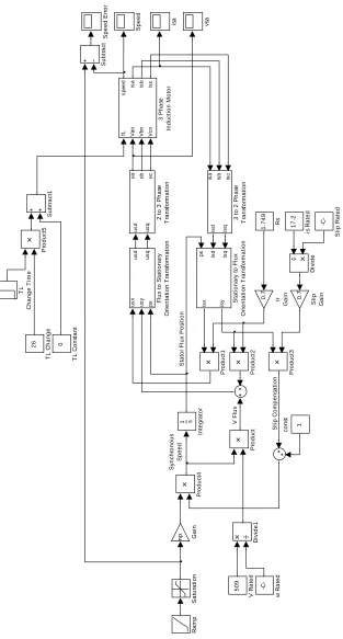
TUFigure 8.2 Experimental VSD SimulinkUPU ® UPU ModelUT...53

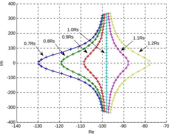
TUFigure 9.1 Rotor Current Poles for Equal Rs Compensation and Zero Slip CompensationUT...58

TUFigure 9.2 Stator Current Poles for Equal Rs Compensation and Zero Slip CompensationUT...58

UTFigure 9.3 Stator Current Poles for Slip Compensation and Zero Rs CompensationT ...59U UTFigure 9.4 Combined Root Locus for Small Signal Stability Analysis in Table 9.2T65U TUFigure 9.5 3D Unstable Conditions for Small Signal Stability Analysis in Table 9.2T ...65U TUFigure 9.6 Unstable Conditions for Small Signal Stability Analysis in Table 9.2UT....66

TUFigure 9.8 Combined Locus for Small Signal stability Analysis in Table 9.2 with

Rsx & Rsy ZeroUT...67

TUFigure 9.9 Experimental VSD Start-up, 80% Torque, 150 rad/sUT...68

TUFigure 9.10 Simulation, Start-up, Zero Torque, 150 rad/sUT...70

TUFigure 9.11 Simulation, Start-up, 80% Rated Torque, 150 rad/sUT...71

TUFigure 9.12 Simulation, Start-up, Zero Torque, 30 rad/sUT...72

TUFigure 9.13 Simulation, Start-up, 80% Rated Torque, 30 rad/sUT...73

TUFigure 9.14 Simulation, Load Change, 0-100% Rated Torque, 150 rad/sUT...74

TUFigure 9.15 Simulation, Load Change, 0-100% Rated Torque, 30 rad/sUT...75

List of Tables

TUTable 3.1 Reference FramesUT...11

TUTable 5.1 Test Bed IM Nameplate DataUT...25

TUTable 5.2 IM Parameter TestUT...27

TUTable 5.3 IM Electrical ParametersUT...27

TUTable 5.4 Generator Friction Coefficient Test DataUT...29

TUTable 5.5 Motor-Generator ParametersUT...31

TUTable 5.6 DOL Start Test - RecordingsUT...32

TUTable 5.7 Sudden Removal of Load Test - RecordingsUT...34

TUTable 5.8 Sudden Application of Load Test – RecordingsUT...34

TUTable 5.9 DOL Start - Simulated and Recorded DataUT...36

TUTable 5.10 Sudden Removal of Load - Simulated and Recorded DataUT...37

TUTable 5.11 Sudden Application of Load - Simulated and Recorded DataUT...38

TUTable 9.1 Motor Details for VSD Stability and Performance EvaluationUT...55

TUTable 9.2 Small Signal Stability Analysis ParametersUT...64

TUTable 9.3 Simulated Performance Criteria, Start-up, Zero Torque, 150 rad/sUT...70

UTTable 9.4 Simulated Performance Criteria, Start-up, 80% Rated Torque, 150 rad/sT ...71U TUTable 9.5 Simulated Performance Criteria, Start-up, Zero Torque, 30 rad/sUT...72

UTTable 9.6 Simulated Performance Criteria, Start-up, 80% Rated Torque, 30 rad/sT.73U TUTable 9.7 Simulated Performance Criteria, Load Change 0-100% Rated Torque, 150 rad/sUT...74

TUTable 9.8 Simulated Performance Criteria, Load Change 0-100% Rated Torque, 30 rad/sUT...75

Nomenclature

Principle Symbols

a Rotational operator, ej2 3π

r

i Rotor current vector, A

, ,

a b c

i i i Instantaneous rotor phase currents in rotor reference frame, A

, ,

ra rb rc

i i i Instantaneous rotor phase currents in rotor reference frame, A

,

r r rd rq

i i Direct and quadrature components of rotor current vector in rotor

reference frame, A ,

s s rd rq

i i Direct and quadrature components of rotor current vector in stator

reference frame, A ,

s s

rd rq

iψ iψ Direct and quadrature components of rotor current vector in stator

flux reference frame, A ,

rx ry

i i Real and imaginary components of vector current vector in stator flux

reference frame, A

s rated

I Stator current magnitude at rated power and speed.

s

i Stator current vector, A

, ,

A B C

i i i Instantaneous stator phase currents in stator reference frame, A

, ,

sA sB sC

i i i Instantaneous stator phase currents in stator reference frame, A

,

s s sd sq

i i Direct and quadrature components of stator current vector in stator

reference frame, A ,

s s

sd sq

iψ iψ Direct and quadrature components of stator current vector in stator

flux reference frame, A ,

sx sy

i i Real and imaginary components of stator current vector in stator flux

reference frame, A

J Mass moment of inertia, kg.mP

2

P

r

J Rotor mass moment of inertia, kg.mP

2

m

L Mutual inductance in the equivalent circuit, H/ph T

r

L Rotor inductance in the Tequivalent circuit, H/ph

lr

L Rotor leakage inductance, H/ph

s

L Stator inductance in the Tequivalent circuit, H/ph

ls

L Stator leakage inductance, H/ph

r

N Number of turns in rotor winding (per phase)

s

N Number of turns in stator winding (per phase)

p Differentiation operator, d

dt

s

R Stator resistance in the Tequivalent circuit, Ω/ph

r

R Rotor resistance in the Tequivalent circuit, Ω/ph

S Rotor slip

rated

S Rotor slip at rated torque and speed

e

T Electromagnetic torque, N.m

L

T Load torque, N.m

r

u Rotor voltage vector, V

,

r r

rd rq

u u Direct and quadrature components of rotor voltage vector in rotor

reference frame, V ,

s s

rd rq

u u Direct and quadrature components of rotor voltage vector in stator

reference frame, V ,

s s

rd rq

uψ uψ Direct and quadrature components of rotor voltage vector in stator

flux reference frame, V ,

rx ry

u u Real and imaginary components of rotor voltage vector in stator flux

reference frame, V

s

u Stator voltage vector, V

, ,

sA sB sC

u u u Instantaneous stator phase voltages, V

,

s s

sd sq

u u Direct and quadrature components of stator voltage vector in stator

,

s s

sd sq

uψ uψ Direct and quadrature components of stator voltage vector in stator

flux reference frame, V ,

sx sy

u u Real and imaginary components of stator voltage vector in stator flux

reference frame, V

r

ψ Rotor flux vector, Wb

,

s s

rd rq

ψ ψ Direct and quadrature components of rotor flux vector in stator reference frame, Wb

,

s s

rd rq

ψ ψ

ψ ψ Direct and quadrature components of rotor flux vector in stator flux reference frame, Wb

,

rx ry

ψ ψ Real and imaginary components of rotor flux vector in stator flux reference frame, Wb

s

ψ Stator flux vector, Wb

, ,

sA sB sC

ψ ψ ψ Stator phase fluxes, Wb ,

s s

sd sq

ψ ψ Direct and quadrature components of stator flux vector in stator reference frame, Wb

,

s s

sd sq

ψ ψ

ψ ψ Direct and quadrature components of stator flux vector in stator flux reference frame, Wb

,

sx sy

ψ ψ Real and imaginary components of stator flux vector in stator flux reference frame, Wb

p

n Number of pole pairs

ms

ω Motor synchronous speed, rad/s

r

ω Rotor angular speed, rad/s

σ Leakage parameter

r

θ Angular position of rotor, rad

Subscripts

A,B,C Stator phase A, phase B, phase C a,b,c Rotor phase a, phase b, phase c

q Quadrature axis

0 Zero sequence

x Real axis in stator flux reference frame

y Imaginary axis in stator flux reference frame

s Stator r Rotor L Load

Superscripts

r Rotor reference frame s Stator reference frame

r

ψ Rotor flux reference frame

s

ψ Stator flux reference frame

Abbreviations

AC Alternating Current

DC Direct Current

CSI Current Source Inverter FOC Field Orientation Control IM Induction Motor

1. Introduction

1.1 Background

In the past DC motors have been prominently used in variable speed drives (VSD) as the torque and flux of these motors can be easily regulated by controlling the armature and field currents of the motor with methods such as the Ward-Leonard system. With the development of semiconductor technology, variable frequency converters emerged and AC induction motor VSDs became available which are now capable of replacing DC drives in many applications.

AC induction motor VSDs have been replacing DC drives as AC induction motors provide operational benefits over DC motors. Due to the constructional aspects of DC motors they require periodic maintenance and have operational limitations such as speed and environmental considerations. AC induction motors on the other hand are more robust then DC motors, require little or no maintenance and generally overcome the operational limitations of DC motors. However, AC induction motor speed control is difficult to implement as the torque and the flux of the motor can not be directly controlled as in the DC motor variable speed drive system.

In AC induction motor drives only the stator voltages and currents can be directly controlled. Therefore a control technique is required to deduce and control the torque and flux of the induction motor. Field orientation control (FOC) as formulated by Blachke (1972) is a technique in which the flux orientation in the motor is used to deduce the torque and flux producing currents of the stator. Therefore the torque and flux of the motor can be controlled and used to control the speed of the motor. Field orientation control has only become practical since the implementation of cost effective power electronics and microprocessor controls.

Scalar control techniques are less complicated and generally less expensive to implement but their performance is generally inferior to that of full vector control.

Open-loop scalar control techniques are generally the least expensive to implement as no motor speed sensor is required. These techniques are likely to prevail in applications where instantaneous speed and position control of induction motors is not critical. Such applications may include pumps, fans and conveyors. Open loop scalar control techniques usually only require feedback of the motor stator currents and are the methods that are considered within this dissertation.

In the research and development of AC induction motor VSD technology the physical implementation of experimental AC induction motor VSDs is not always practical due to the physical resources that are required. To overcome this the operation of experimental drives can be simulated by developing and implementing a model of the VSD. These models can be implemented in programs such as MatlabP

®

P and SimulinkP

®

P

and allow the performance of the system to be analysed without access to physical resources.

1.2 Aim and Objectives of the Project

The general aim of this project is to implement a model for an AC variable speed drive for induction motors and to use this model to determine the limits of stability. The objectives of this project as defined in the project specification are:

1. Develop a state space model for the standard three phase induction motor. State variables can be either direct-axis and quadrature-axis currents or direct-axis and quadrature-axis flux linkages or a combination of currents and flux linkages.

2. Implement the model in (1) using SimulinkP

®

P

and simulate:

a. DOL start-up from rest.

b. Sudden application of mechanical load with the motor initially operating at steady-state speed on no-load.

3. Design and carry out physical tests to verify some of the predictions of step (2).

4. Develop a state-space model for an AC variable speed drive that consists of the induction motor model in (2), slip compensation and stator resistance voltage drop compensation.

5. Implement the model in (4) using SimulinkP

®

P

and analyse the performance and stability of the drive.

In setting the above objectives the focus has been on low complexity speed control schemes that provide a mid range performance and can be implemented on low cost systems.

1.3 Outline of Dissertation

In this dissertation the reader is presented with the basic theory of AC induction motors and AC variable speed drives before the experimental drive is developed and the performance and stability of the drive is analysed.

Chapters 2 to 5 cover induction motor operation and modelling. In chapter 2 the principles of the induction motor are presented before the 2-phase model of the induction motor is developed in chapter 3. In chapter 4 a SimulinkP

®

P model of the

induction motor is developed and then verified in chapter 5. The verification consists of induction motor tests and comparison of test results and simulations.

Chapters 6 to 8 cover variable speed drive operation, development of the experimental drive and modelling of the drive. In chapter 6 the principles of AC variable speed drives are presented before the experimental drive is developed in chapter 7. In chapter 8 a SimulinkP

®

P model of the experimental drive and a constant V/f drive are developed.

2.

Principles of Induction Motors

2.1 Construction

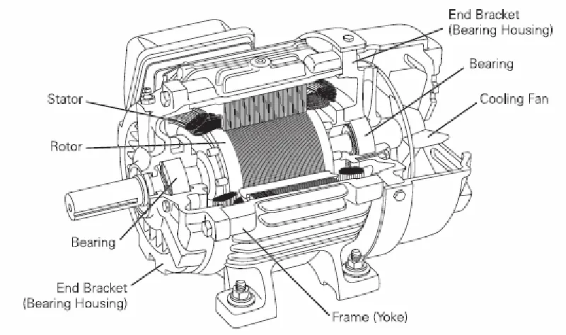
Induction motors consist of a stationary frame referred to as the stator and a rotating frame referred to as the rotor. The stator is housed in a frame onto which mounting feet are attached for securing the machine and bearing housings are attached for supporting the rotor. Both the stator and rotor carry windings which are magnetically coupled across the air gap in the machine.

The stator is an annular steel frame which carries distributed windings in slots on its inner surface. In three phase IMs the stator windings are arranged in coil groups with even spacing around the stator so that a rotating magnetic field is generated by the three phase supply.

The rotor of IMs can be of wound rotor construction or squirrel-cage construction. Wound rotor constructions consist of a cylindrical steel frame which carries distributed windings in slots on its outer surface. This type of construction usually incorporates slip rings so that external resistances can be inserted into the rotor circuit to modify the torque characteristics of the motor.

[image:18.595.113.513.58.295.2]

Figure 2.1 Induction Motor Construction

(source: http://www.sea.siemens.com/step )

2.2 Operation

The electrical operation of the IM is simular to that of an electrical transformer where the stator windings form the primary winding and the rotor windings form the secondary winding. The application of alternating currents to the 3 phase stator windings produces a rotating magnetic field through the air gap and the rotor. The speed at which this stator magnetic field rotates is referred to the synchronous speed of the motor. If the rotor is not rotating at a speed equal to synchronous speed then the stator magnetic field will produce an alternating flux in the rotor. By Faraday’s law, this alternating flux will produce currents in the rotor windings and the resultant interaction between the rotor current and the flux will produce a force. As the rotor is mounted on a shaft this force will cause the rotor to rotate if friction and the torque of the load is overcome.

must exist for a rotational torque to be produced. This difference between synchronous and rotor speeds is referred to as slip.

2.3 Dynamic

Equations

In symmetrical IMs all phases are identical and distributed equally within the machine. Therefore the phase parameters across all phases are identical. If a symmetrical IM is operated from a symmetrical power supply then the magnitude of the voltage, current and flux phasors in each phase are also identical and the analysis of the symmetrical IM is greatly simplified. Each winding of an IM can be represented by a resistance and an inductance in series, which forms the circuit in Figure 2.2, when the windings are connected in Wye configuration.

Figure 2.2 Wye Induction Motor Equivalent Circuit

A s A

d u R i

dtψA

= + (2.1)

B s B

d u R i

dtψB

= + (2.2)

C s C

d u R i

dtψC

= + (2.3)

0

a r a a

d u R i

dtψ

= + = (2.4)

0

b r b b

d u R i

dtψ

= + = (2.5)

0

c r c c

d u R i

dtψ

= + = (2.6)

The magnetic flux in the stator or rotor windings of the IM is a summation of magnetic fluxes produced within the winding and the mutual coupling of magnetic fluxes from the other stator and rotor windings, which is dependant upon the mutual inductances between the windings. Using the phase current and mutual inductances the magnetic flux in each winding is given by (2.7) to (2.12).

A L iAA A L iAB B L iAC C L iAa a L iAb b L iAc c

ψ = + + + + + (2.7)

B L iBA A L iBB B L iBC C L iBa a L iBb b L iBc c

ψ = + + + + + (2.8)

C L iCA A L iCB B L iCC C L iCa a L iCb b L iCc c

ψ = + + + + + (2.9)

a L iaa a L iab b L iac c L iaA A L iaB B L iaC C

ψ = + + + + + (2.10)

b L iba a L ibb b L ibc c L ibA A L ibB B L ibC C

ψ = + + + + + (2.11)

c L ica a L icb b L icc c L icA A L icB B L icC C

ψ = + + + + + (2.12)

[image:21.595.112.320.54.273.2]

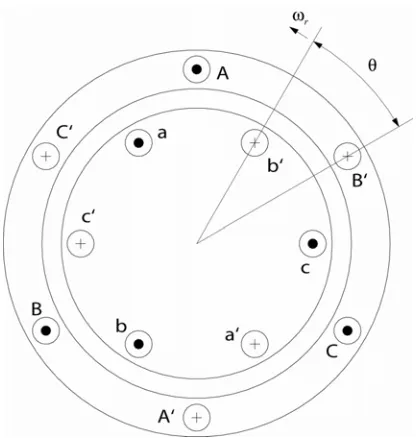
Figure 2.3 Winding Distribution

The mutual inductances in the winding flux equations of (2.7) to (2.12) can be represented by fixed inductances and inductances as functions of angular displacement as given in (2.13) to (2.19).

s AA BB CC

L =L =L =L (2.13)

r aa bb

L =L =L =L_cc (2.14)

ss AB AC BC BA CA CB

M =L =L =L =L =L =L (2.15)

rr ab ac bc ba ca cb

M =L =L =L =L =L =L (2.16)

cos

sr Aa aA Bb bB Cc cC

M θ =L =L =L =L =L =L (2.17)

cos( 120 )

sr Ab bA Bc cB Ca aC

M θ+ ° =L =L =L =L =L =L (2.18)

cos( 240 )

sr Ac cA Ba aB Cb bC

M θ+ ° =L =L =L =L =L =L (2.19)

(

cos( ) cos( 120 ) cos( 240 )

)

A L is A M iss B M iss C Msr ia ib ic

ψ = + + + θ + θ+ ° + θ+ ° (2.20)

(

cos( 240 ) cos( ) cos( 120 )

)

B M iss A L is B M iss C Msr ia ib ic

ψ = + + + θ + ° + θ + θ+ ° (2.21)

(

cos( 120 ) cos( 240 ) cos( )

)

C M iss A M iss B L is C Msr ia ib ic

ψ = + + + θ+ ° + θ + ° + θ (2.22)

(

cos( ) cos( 120 ) cos( 240 )

)

a L ir a M irr b M irr c Msr iA iB iC

ψ = + + + θ + θ + ° + θ + ° (2.23)

(

cos( 240 ) cos( ) cos( 120 )

)

b M irr a L ir b M irr c Msr iA iB iC

ψ = + + + θ + ° + θ + θ+ ° (2.24)

(

cos( 120 ) cos( 240 ) cos( )

)

c M irr a M irr b L ir c Msr iA iB iC

3.

2 Phase Model of Induction Motors

3.1 Reference

Frames

Reference frames of IMs are the spatial orientations that are used as a reference for defining quantities. For example the induction motor dynamic equations in chapter 2.3 had stator and rotor quantities referenced to the physical location of the windings within the stator and rotor. Therefore cosine terms were required to transform the rotor quantities to the stator and vice-versa.

IM references frames are defined with respect to rotational references, which vary in rotational speed. In this dissertation the reference frame is denoted by the superscript applied to quantities. The four common reference frames used in IMs are given in Table 3.1.

Table 3.1 Reference Frames

Frame Reference Superscript

Stator (Stationary) Stator S

Stator flux (Synchronous) Stator flux vector ψ_s

Rotor Rotor R

Rotor flux Rotor flux vector ψ_r

Figure 3.1 Reference Vectors

The space vectors can be transformed between reference frames by using the rotational operator j r

eθ and the turns ratio of the stator to rotor windings. The transformation of

the rotor currents from the rotor to the stator reference frames is given in (3.1).

j r

s r

r

e i

v

θ

= i_r (3.1)

where:

s

r

N v

N

=

3.2 3 to 2 Phase Transformation

3 to 2 phase transformations are used to transform quantities in 3 phase machines to equivalent quantities in a two phase machine. These transformations are useful in IM models as the models can be formulated with two phases which reduces the complexity of the model and aids with analysis and control.

using a rotational operator to sum the instantaneous 3 phase quantities. The space vector is then resolved into real and imaginary parts to obtain two orthogonal

quantities as shown in Figure 3.2 for the stator voltage.

Figure 3.2 IM Field Orientation

The 3 to 2 phase transformation of stator voltages are demonstrated in the following and is the same process for currents and fluxes. The space vector of the stator voltage is obtained from the 3 phase voltages using (3.2). The space vector is then resolved into real and imaginary components as in (3.3). The voltage component on the real axis is referred to as the direct axis voltage and component on the imaginary axis is referred to as the quadrature component.

2

s s s s

s sA sB sC

u =u +au +a u (3.2)

s s s

s sd sq

u =u + ju

)

(3.3)

where:

sd

u =direct axis voltage

sq

u =quadrature axis voltage

The two phase components can be directly obtained from the 3 phase components by using (3.4) and (3.5).

( )

(

2 (1) (2) (0)

Re( )

cos 120 cos 240

1 1

2 2

s

sd sA sA sA

s s s

sA sB sC

s s s

sA sB sB

u u au a u

u u u

u u u

= + +

= + +

= − −

)

(3.4)

( )

(

2 (1) (2) (0)

Im( )

sin 120 sin 240

3 3

2 2

s

sq sA sA sA

s s

sB sC

s s

sB sB

u u au a u

u u

u u

= + +

= +

= −

(3.5)

From (3.4) and (3.5), the 3-2 phase transformation matrix is formed. The zero sequence voltage, s₀

s

u is also included in this matrix to form a square matrix so that the inverse

transformation matrix can be obtained from direct inversion of the transformation matrix. For balanced three phase operation of a symmetrical machine the sum of the stator voltage phasors is equal to zero, so s₀

s

u is equal to zero and has no affect on the

3-2 phase transformations. The 3-3-2 phase and 3-2-3 phase transformations are given in (3.6) and (3.7). Q is the 3-2 transformation matrix and 1

Q− is the 2-3 transformation

matrix.

0 s s sd s s s sq sB s s s s u u

u Q u

u u ⎡ ⎤ ⎡ ⎤ ⎢ ⎥₌ ⎢ ⎥ ⎢ ⎥ ⎢ ⎥ ⎢ ⎥ ⎢ ⎥ ⎣ ⎦ ⎣ ⎦ A C (3.6) 1 0 s s sA s s d s sB s s sC s u u

u Q u

u u − ⎡ ⎤ ⎡ ⎢ ⎥₌ ⎢ ⎢ ⎥ ⎢ ⎢ ⎥ ⎢ ⎣ ⎦ ⎣ sq ⎤ ⎥ ⎥ ⎥⎦ (3.7) where: 1 1 1 2 2 3 3 0 2 2

1 1 1

Q ⎡ _{− −} ⎤ ⎢ ⎥ ⎢ ⎥ ⎢ ⎥ =_⎢ − _⎥ ⎢ ⎥ ⎢ ⎥ ⎢ ⎥ ⎣ ⎦ 1 2 1 0 3 3

1 1 1

3 3 3

1 1 1

3 3 3

Q− ⎡ ⎤ ⎢ ⎥ ⎢ ⎥ ⎢ ⎥ = −_{⎢ ⎥} ⎢ ⎥ ⎢_{− −} ⎥ ⎢ ⎥ ⎣ ⎦

The product of the 2 phase currents and voltages is proportional to the product of the 3 phase currents and voltages by a factor of 2/3 as given in (3.8). Therefore the power in the 3 phase motor is 2/3 the power in the 2 phase motor as given by (3.9).

1 2

3

T

S T S s s S T S

sABC sABC sdq sdq sdq sdq

u i =⎡_⎣Q u− ⎤_⎦ Qi = u i (3.8)

where:

1 s T s T 1

sdq sdq

Q u− u Q−

⎡ ⎤ =⎡ ⎤ ⎡

⎣ ⎦ ⎣ ⎦ ⎣ ⎤⎦T

2 3

ABC dq

3.3 Development of 2 Phase Model

The 2 phase model of the induction motor is developed from the dynamic equations of the induction motor in chapter 2.3. Using vector quantities, the stator and rotor voltages are given by the dynamic equations (3.10) and (3.11).

s

s s s s

s s s

d u R i

dt

ψ

= + (3.10)

r

r r r r

r r r

d u R i

dt

ψ

= + (3.11)

(3.10) is referenced to the stator reference frame and (3.11) is referenced to the rotor reference frame. (3.11) can be transformed to the stator reference using a rotational operator as in (3.12). The dynamic equation of the rotor voltage referenced to the stator is then (3.13).

0 0 0

j j j

s s s s

r r r

e e d e

u R i

v v dt v

θ θ θ

r ψ

− − _⎛ − _⎞

= + _⎜

⎝ ⎠⎟ (3.12)

s

s s s r s s

r r r r

d

u R i j

dt

ψ

r ω ψ

= + − (3.13)

where:

s

r

N v

N

= ,turns ratio of stator and rotor windings

0 j

eθ , rotational operator

The voltage equations in the stator reference frame are then given by (3.14) and (3.15).

s s s s

s s s s

u =R i +pψ (3.14)

( )

s s s s s

r r r r

where:

d p

dt

= ,differential operator

The flux linkages in the stationary stator reference frame can be expressed by the flux linkage equation (3.16).

s s s m s s s s m r r r

L L i

L L i

ψ ψ ⎡ ⎤ ⎡ ⎤⎡ = ⎢ ⎥ ⎢ ⎥⎢ ⎣ ⎦ ⎣ ⎦ ⎣ ⎤ ⎥

⎦ (3.16)

Combining the flux linkage equation (3.16) and the voltage equations (3.14) and (3.15) forms the matrix equation (3.17) for the voltages in the stationary stator reference frame.

( ) ( )

s

s s

s s m

s

s s

s

s s

r m r r r

r r

R pL pL

u i

p j L R p j L

u ω ω i

⎡ ⎤

⎡ ⎤ + ⎡ ⎤

= ⎢

⎢ ⎥ _{− + −} ⎢ ⎥

⎣ ⎦ ⎣ ⎦⎥⎣ ⎦ (3.17)

By breaking the voltage and current vectors into to the orthogonal components ‘d’ and ‘q’, equation (3.17) can be written as (3.18). After isolating the derivatives (3.18) can be written as (3.19). Note all the parameters are referred to the stator reference frame so the superscript ‘s’ has been omitted for the remaining model development.

0 0

0 0

sd s s m sd

sq s s m sq

rd m r m r r r r rd

rq r m m r r r r rq

u R pL pL i

u R pL pL i

u pL L R pL L i

u L pL L R pL i

ω ω ω ω + ⎡ ⎤ ⎡ ⎤⎡ ⎢ ⎥ ⎢ ₊ ⎥⎢ ⎢ ⎥₌⎢ ⎢ ⎢ ⎥ ⎢ + ⎥⎢ ⎢ ⎥ ⎢ _{− − +} ⎥⎢ ⎢ ⎥ ⎣ ⎦⎢ ⎣ ⎦ ⎣ ⎤ ⎥ ⎥ ⎥ ⎥ ⎥ ⎥⎦ (3.18)

0 0 0 0 0

0 0 0 0 0

0 0

0 0 0

0

sd s sd s m sd

sq s sq s

rd r m r r r rd m r rd

rq r m r r r rq m r rq

u R i L

u R i L d

u L R L i L L dt

u L L R i L L

By using matrix inversion the derivatives of the currents can be isolated in (3.19). Assuming that the closed loop rotor voltages are zero the system can be arranged to produce (3.20) which is the 2 phase ‘dq’ state space model of the induction motor. This model is used in many publications.

2

2

s r m m r r m

s r s r s s

sd _{r m s r m m r} sd

sq _{r s s s r s} sq

rd _{m s r m r r} rd

rq r s r r rq

r m m s r r

r r s r

R L L R L

L L L L L L

i _{L R L L R} i

i _{L L L L L L} i

d

i i

dt L R L R

i _{L L L L} i

L L R R

L L L L

ω ω

σ σ σ σ

ω ω

σ σ σ σ

ω ω

σ σ σ σ

ω ω

σ σ σ σ

⎡ ⎤ − ⎢ ⎥ ⎢ ⎥ ⎢ ⎥ ⎡ ⎤ ⎡ ⎤ − − − ⎢ ⎥ ⎢ ⎥ ⎢ ⎥ ⎢ ⎥ ⎢ ⎥_{= ⎢} ⎢ ⎥ ⎥ ⎢ ⎥ ⎢ ⎥ ⎢ − − − ⎥ ⎢ ⎥ ⎢ ⎥ ⎢ ⎥ ⎢ ⎥⎢ ⎥ ⎣ ⎦ ⎣ ⎦ ⎢ ⎥ ⎢ − ⎥ ⎢ ⎥ ⎣ ⎦ 1 0 1 0 0 0 s sd s sq m r s m r s L u L u L L L L L L σ σ σ σ ⎡ ⎤ ⎢ ⎥ ⎢ ⎥ ⎢ ⎥ ⎢ _{⎥ ⎡ ⎤} ⎢ ⎥ + _{⎢ ⎥} ⎢ _{⎥ ⎣ ⎦} − ⎢ ⎥ ⎢ ⎥ ⎢ ⎥ − ⎢ ⎥ ⎣ ⎦ (3.20) where: 2 1 m r s L L L

σ = − ,leakage parameter

The state space model (3.20) is for a 2 pole machine ( = 1). Therefore the rotor speed,

p

n

r

ω in the state space model is the speed of an equivalent two pole machine. The real and model rotor speeds are related as in (3.21).

(

r P r real)

ω η ω= (3.21)

sin( )

e rs r

T′ =ψ i δ (3.22)

where:

δ = Angular displacement between stator and rotor reference frames

rs L im s

ψ = ,flux linking the rotor due to stator current

The sine of the angular displacement between the stator linkage flux vector and the rotor current vector is given by:

(

)

sin( ) sin( )

sin( ) cos( ) cos( )sin( ) 1

s r

s r s

sq rd sd rq s r

i i i i

i i

r

δ θ θ

θ θ θ

= −

= −

= −

θ

By substituting the above relationship into (3.22) the 2 phase, 2 pole electromagnetic torque can be determined from currents only. Multiplying this by the number of pole pairs gives the electromagnetic torque produced by a 2 phase, multi-pole pair motor. As the power in the 2 phase and 3 phase motors is related by a factor of 2 3as given in (3.9), the actual 3 phase electromagnetic torque is given by (3.23).

2 ( 3

e p m sq rd sd rq

T =n L i i −i i ) (3.23)

Subtracting the load and friction torque from the electromagnetic toque and dividing by the rotor moment of inertia gives the acceleration of the rotor as in (3.24).

1 (

r

e L r

d

T T f

dt J )

ω _ω

4.

Implementation of IM Model in Simulink

P

®

P

4.1 IM

Simulink

P

®

P

Model

The 2 phase IM model developed in chapter 3.3 has been implemented in SimulinkP

®

P so

that the operation of the induction motor can be simulated. The IM model has been implemented as a function block which has the stator voltages and load torque as inputs and the stator currents and rotor speed as outputs. The parameters of the IM are defined in the SimulinkP

®

P model by their respective symbols and are set by assigning their

numerical values in the MatlabP

®

P workspace. This allows the model to be used for the

simulation of any induction motor.

The IM state space equation (3.20) is the basis for the model and is used to calculate the stator and rotor currents of an equivalent 2 phase, 2 pole motor. Each line of the IM state space model has been implemented in separate sub-function blocks. For the stator direct phase current the relevant line from the state space equation is given by (4.1) and the SimulinkP

®

P sub-function block is given Figure 4.1.

2 ₁

0

sd

sq

sd s r m m r r m

rd sq

s r s r s s s

rq

i

i u

di R L L R L

i u

dt L L L L L L L

i

ω ω

σ σ σ σ σ

⎡ ⎤ ⎢ ⎥

sd

⎡ ⎤

⎡ ⎤_{⎢ ⎥} ⎡

= −_{⎢ ⎥} +_⎢ ⎤_{⎢ ⎥}

⎢ ⎥

⎣ ⎦_{⎢ ⎥} ⎣ ⎥⎦ ⎣ ⎦

⎢ ⎥ ⎣ ⎦

di/dt

1

isd

Sum of Elements1

Product3 Product1

1 s

Integrator

-K-Gain4

-K-Gain3

-K-Gain2

-K-Gain1

-K-Gain

5

usd

4

wr 3

irq 2

ird 1

isq

Figure 4.1 Stator Direct Phase Sub-Function Block

From the 2 phase, 2 pole stator and rotor currents the 3 phase multi-pole electromagnetic torque is calculated by implementing equation (3.23) within another sub-function block as given in Figure 4.2.

Electromagnetic Torque Evaluation

2 Phase Torque

3 Phase Torque

1

Te

Product1 Product

np

Gain2

2/3

Gain1 Lm

Gain Add

4

irq 3

ird 2

isq

1

isd

The 3 phase voltage inputs to the model are transformed to 2 phase values and the stator 2 phase currents are transformed to 3 phase values using the 3-2 and 2-3 phase transformation blocks shown in Figure 4.3 and Figure 4.4. These blocks implement the 3-2 and 2-3 phase transformations defined in chapter 3.2.

3 to 2 phase transformation

Stator Reference Frame

2

usq 1

usd

-K-Gain4

-K-Gain3

-K-Gain2

-K-Gain1

Add2 Add1

3

Vcn 2

Vbn 1

Van

Figure 4.3 Stator Voltage 3-2 Transformation Sub-Function Block

2 to 3 phase transformation

Stator Reference Frame

3

ic 2

ib 1

ia

-K-Gain5

-K-Gain4 1/3

Gain3 1/3

Gain2 2/3

Gain1

Add2 Add1 2

iqs 1

ids

In the complete model the motor acceleration torque is determined by subtracting the load and friction torque from the electromagnetic torque. Dividing the acceleration torque by the rotor moment of inertia then gives the acceleration of the rotor which is passed through an integral block to obtain the rotor speed. The rotor speed is multiplied by the number of pole pairs to obtain the equivalent 2 phase, 2 pole rotor speed which is fed back to the phase current sub-function blocks for subsequent current calculations. The complete IM SimulinkP

®

P

Induc ti on M o to r M o d e l In S tat o r R e fe re nc e F ram e w it h R o to r and S tat or C u rr ent s as S ta te V a ri a b le s Ac c e le ra ti o n To rq u e Ac c e le ra ti o n 3 P h as e S pee d 2 P has e Sp ee d

4 _isc 3 _isb 2 _isa

1

sp

eed

is

d

ird irq wr us

q is q is q is q

ird irq wr us

d is d is d is d is q

ird wr us

q irq ir q is d is q

irq wr us

d ird ir d S a tu ra ti o n 1 s In tegr at or np Ga in 1 1/

J _Gain

f F ri c ti on T o rque is d is q ir d ir q Te E le c tr om agne ti c T o rque A dd1 Va n Vb n Vc n us d us q 3 t o 2 P has e T ra n sf or m a ti on id s iq s is a is b uc 2 t o 3 P has e T rans fo rm at io n 4 Vc n 3 Vb n 2 Va n 1 _TL

Figure 4.5 IM SimulinkP

5.

Verification of IM Model

5.1 Testing and Model Verification

The ability of the induction motor model to accurately simulate the operation of the real induction motor is required to be determined so that the validity of simulations can be verified and the reliable application of the model can be determined.

Verification of the model has been performed by comparing simulations of induction motor operation to recordings of the real induction motor operation. This has been performed for direct online starting and load variations with the motor initially operating at steady state speed.

The testing of a real induction motor was performed on a motor-generator unit with a resistive load bank. The drive motor was a 4 kW squirrel cage induction motor with coupling to the DC generator. The coupling could be disengaged so that stand alone induction motor operation could be achieved. The nameplate data of the IM in the test bed is given in Table 5.1 and the test bed is shown in Figure 5.1.

During testing voltages and currents were recorded with a 4 channel storage oscilloscope using current and voltage probes. The length of recording was limited by the maximum oscilloscope storage of 500 data entries.

Table 5.1 Test Bed IM Nameplate Data

Voltage 415 V

Frequency 50 Hz

Current 8.1 A

Power 4 KW

Speed 1420 RPM

Figure 5.1 IM Test Bed

5.2 Parameter Testing of IM

Testing was performed on the motor-generator set to determine the friction coefficients and the moment of inertia of the complete unit. These are required for simulation. The induction motor electrical parameters were obtained from testing performed during previous laboratory work in practical courses.

Table 5.2 IM Parameter Test

No Load Test

Phase voltage, V_P- V_rms 227

Line current , I_L - A_rms 2.98

Input power, P - W 340

Input apparent power, S - KVA

{

3I VL P

}

2029.38 Rotor speed - RPM / rad.sP

-1

P 1500 / 157.08

Power factor angle, θ - degrees

{

cos−1

(

P S

)

}

80.36 Magnetising current, I_m - A

{

sin( )θ I_L

}

2.934 Magnetising reactance, X_m - Ω

{

V_P I_m

}

j77.37 Magnetising inductance, L_m - h

{

X_m (2πf)

}

0.246

Locked Rotor Test

Phase Voltage, V_P- V_rms 49.07

Line Current, I_L - Arms 8.1

Input power, P - W 648

Input apparent power, S - KVA

{

3I VL P

}

1192 Power Factor Angle, θ - degrees

{

cos−1

(

P S

)

}

57.07 Phase Impedance, Z- Ω

{

V_P I_L

}

6.058 Resistance, R- Ω

{

Zcos( )θ

}

3.293 Reactance, X - Ω

{

Zsin( )θ

}

j5.084 Inductance, – H L

{

X (2π f)

}

0.0162

DC Stator Test

Stator resistance, R_s- Ω 1.749

Table 5.3 IM Electrical Parameters

Stator resistance, R_s- Ω 1.749

Rotor resistance, R_r – Ω

{

R−R_s

}

1.544 Stator leakage inductance, L_ls - H

{ }

L 2 0.0081 Rotor leakage inductance, L_lr - H

{ }

L 2 0.0081

Mutual inductance, L_m - H 0.246

can then be determined using (5.3) which includes all loses other then stator resistance loss as a function of rotor speed.

r

e L m m

d

T T J f

dt r

ω _ω

= + + (5.1)

where:

m

f = friction coeficient of motor

2

in m r Loss

P = f ω +P (5.2)

2 2 3

in s s

m

r

P I R f

ω

−

= (5.3)

Using the no load test data from Table 5.2 and (5.3), the friction coefficient of the induction motor was determined to be 0.012 Nm.s.radP

-1

P.

The torque relationship of the motor-generator set is described by (5.4). For steady state operation with no generator load the speed is constant and the power relationship within the motor can be described by (5.5).

out

r r

e m m r g g r

r

P

d d

T J f J f

dt dt

ω _ω ω _ω

ω

− − = + + (5.4)

2

( )

in g m r Loss

P = f + f ω +P (5.5)

2 2 3

in s s

g m

r

P I R

f f

ω

−

= − (5.6)

3 cos ( ) (

in L L ab a ab b

P = V I θ =mean v i +mean v −i ) (5.7)

The data used to calculate the generator friction coefficient is give in below in Table 5.4. From this data the generator friction coefficient was determined to be 0.0277 Nm.s.radP

-1

P.

Table 5.4 Generator Friction Coefficient Test Data

Power input, P_in - W 1040

Stator line current, I_S - A_rms 3.5

Rotor speed – RPM / rad.sP

-1

P 1495 / 156.6

Motor friction coefficient, f_m - Nm.s.radP

-1

P 0.012

Generator friction coefficient, f_g - Nm.s.radP

-1

P 0.0277

Motor - Generator friction coefficient - Nm.s.radP

-1

P 0.0397

To obtain the moment of inertia for the complete motor-generator set, a test with speed transients was required. If the input power to the induction motor is zero then by rearranging (5.4) and integrating to remove the derivative, (5.8) is obtained. The left hand integral of (5.8) can be solved to obtain (5.9) which can be used to determine the combined moment of inertia from data recorded during the run down of the motor-generator set after supply to the induction motor is disconnected.

1 1

2 2

( ) ( )

t

m g r m g r

r t

Ia Ea

J J d f f d

ω

ω

ω

ω

−

+ = − +

∫

∫

ω t (5.8)

1

2 1

( ) ( )

1 2

t

m g m g r

r t

Ia Ea

J J f f ω d

ω ω ω

−

+ = − +

−

∫

t (5.9)

motor speed. The output voltage of the generator is proportional to the motor speed when excitation is held constant and is described by (5.10).

a r

f

V ki

ω = (5.10)

where:

a

f

V generated voltage i field current k generator constant

= = =

To obtain the data for the inertia testing the motor-generator set was operated with a load at steady state. The power to the induction motor was then disconnected and the generator output voltage and current were recorded with the oscilloscope during the rundown of the rotor. The recorded values are plotted in Figure 5.2.

0 1 2 3 4 5 6 7 8 9 10

-50 0 50 100 150 200 250

c

u

rrent

A

/

v

o

lt

ag

e

V

time - s

armature voltage armature current

The data was then exported to MatlabP

®

P where the rotor speed was calculated using

(5.10) and the moment of inertia was calculated by implementing (5.9) with numerical integration. The moment of inertia and the friction coefficients calculated for the motor-generator set are given in Table 5.5.

Table 5.5 Motor-Generator Parameters

Induction motor friction coefficient - Nm.s.radP

-1

P 0.012

Generator friction coefficient - Nm.s.radP

-1

P 0.0277

Motor-generator combined friction coefficient - Nm.s.radP

-1

P

0.0397

Motor-generator combined moment of inertia - kg.mP

-2

P 0.3708

5.3 Verification Testing of IM

To verify the induction motor model, data from a real induction motor was required for comparison with model simulations. Tests were performed to obtain induction motor data during direct on line starting and sudden removal and sudden application of loads.

0 0.02 0.04 0.06 0.08 0.1 0.12 0.14 0.16 0.18 0.2 -80

-60 -40 -20 0 20 40 60 80 100

DOL Start - Ib

time-sec

cu

rr

e

n

t-A

Figure 5.3 DOL Start Test – Stator Line Current

Table 5.6 DOL Start Test - Recordings

Parameter Initial Final

Load: 0 Nm 0 Nm

Speed: 0 157.1 rad/sec

Stator Current: 0 3 A rms

During the sudden removal and application of load to the motor, the motor was engaged to the DC generator and a resistive load was used to apply a load to the DC generator and the motor. A stator current, a stator line voltage, the generator armature voltage and the generator armature current were recorded during the test.

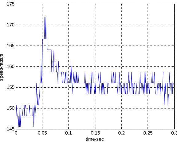
From the generator armature voltage the speed of the motor can be determined using (5.10) but this relationship does not hold during the switching transients in this test, due to the inductive properties of the generator. During the transient period, a speed overshoot is incorrectly indicated by the armature voltage, as shown in Figure 5.4.

0 0.05 0.1 0.15 0.2 0.25 0.3 145

150 155 160 165 170 175

time-sec

s

p

eed

-r

ad

s

[image:45.595.131.419.69.300.2]

/s

Figure 5.4 Sudden Removal of Load Test – Speed Calculated From Armature Voltage

The recorded stator line current for the sudden removal and application of load are shown in Figure 5.5 and Figure 5.6. The recorded data during these tests are given in Table 5.7 and Table 5.8.

0 0.05 0.1 0.15 0.2 0.25 0.3 0.35 0.4 0.45 0.5

-15 -10 -5 0 5 10 15

c

u

rr

e

n

t -

A

Table 5.7 Sudden Removal of Load Test - Recordings

Parameter Initial Final

Generator Load: 3.8 KW 0 W

Speed: 148.6 rad/sec 156.6 rad/sec

Stator Current: 8.4 Arms 3.46 A rms

0 0.05 0.1 0.15 0.2 0.25 0.3 0.35 0.4 0.45 0.5 -15

-10 -5 0 5 10 15

c

u

rr

ent

A

time - sec

Figure 5.6 Sudden Application of Load Test – Stator Current

Table 5.8 Sudden Application of Load Test – Recordings

Parameter Initial Final

Resistive Load: 0 KW 3.85 KW

Speed: 156.6 rad/sec 148.5 rad/sec

Stator Current: 3.46 A rms 8.4 A rms

5.4 Verification of Model

The induction motor model has been verified by comparison of data recorded during the verification testing and simulations using the SimulinkP

®

P induction motor model. This

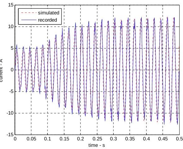
For the direct online start of the motor, the recorded and simulated stator currents are shown in Figure 5.7 and the recorded and simulated data is given in Table 5.9. From this figure it can be seen that the recorded and simulated currents are not the same during fist 4 cycles of the stator current but they are simular after this period. During the first 4 cycles the recorded current is greater then the simulated current. This is due to the relationship between the flux and current becoming non-linear during high currents, due to magnetic flux saturation. The induction motor model is a linear model and does not accommodate this non-linear relationship at high currents.

Magnetic flux saturation within the motor occurs in the leakage and magnetising branches of the induction motor during high currents. During magnetic saturation the rate of change of flux density to the applied current decreases and the effective inductance of the relationship is reduced. Therefore a fixed inductance can only be used to model the flux and current relationship in the linear range. Magnetic saturation in the motor during motor transients is difficult to model as the level of saturation is not constant across all magnetic paths. Therefore each magnetic path needs to be considered separately which significantly increases the complexity of the model. Modelling of the saturation also requires knowledge of the physical arrangement of the motor windings to determine the flux densities.

After the fist 4 cycles of the DOL start the recorded and simulated currents are simular and can be regarded as the same. From Table 5.9, the final steady state recorded currents of the motor are the same and the speeds are simular.

0 0.02 0.04 0.06 0.08 0.1 0.12 0.14 0.16 0.18 0.2 -80

-60 -40 -20 0 20 40 60 80

c

u

rr

e

n

t -

A

time - sec

simulated recorded

Figure 5.7 DOL Start - Simulated and Recorded Stator Current

Table 5.9 DOL Start - Simulated and Recorded Data

Simulated Recorded

Final speed: 156.56 rad/sec 157.1 rad/sec

Final stator current: 3 Arms 3 Arms

0 0.05 0.1 0.15 0.2 0.25 0.3 0.35 0.4 0.45 0.5 -15

-10 -5 0 5 10 15

c

u

rr

en

t -

A

time - s

[image:49.595.138.430.69.306.2]

simulated recorded

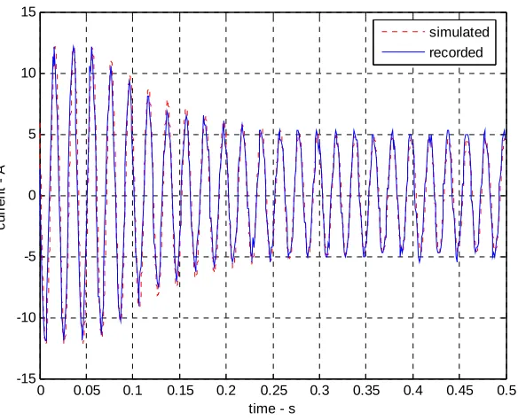
Figure 5.8 Sudden Removal of Load - Recorded and Simulated Stator Current

Table 5.10 Sudden Removal of Load - Simulated and Recorded Data

Simulated Recorded

Initial load: 25 Nm 3.8 Kw / 25 Nm

Final load: 0 Kw 0 Kw

Initial speed: 148 Rad/sec 148.6 rad/sec

Final speed: 155.5 rad/sec 156.6 rad/sec

Initial stator current: 8.42 A rms 8.4 A rms

0 0.05 0.1 0.15 0.2 0.25 0.3 0.35 0.4 0.45 0.5 -15

-10 -5 0 5 10 15

cu

rr

e

n

t

A

time - s simulated

recorded

[image:50.595.134.429.68.308.2]

Figure 5.9 Sudden Application of Load - Recorded and Simulated Stator Currents

Table 5.11 Sudden Application of Load - Simulated and Recorded Data

Simulated Recorded

Initial load: 0 Nm 0 Kw / 0 Nm

Final load: 25.9 Nm 3.85 Kw / 25.9 NM

Initial speed: 155.5 rad/sec 156.6 rad/sec

Final speed: 147.8 rad/sec 148.5 rad/sec

Initial stator current: 3.3 A rms 3.46 A rms

Final stator current 8.46 A rms 8.4 A rms

6.

Principles of AC VSD

6.1 AC VSDs

AC variable speed drives for induction motors are generally of the variable frequency type where the frequency and power of the stator supply are controlled. Other types of variable speed drives include the reduced voltage and rotor resistance types but the variable frequency type is the only type considered in this dissertation as this provides the largest range of operating speed.

The variable frequency type of AC VSDs can be classified into DC-link converter and cycloconverter schemes. The DC-link converter scheme involves the rectification of the AC supply to a DC-link and the inversion of the DC to produce the stator supply at the required frequency and power. Cycloconverter schemes do not have a DC-link and perform direct frequency conversion of the AC supply to the stator supply. Cycloconverter VSDs are generally used in large power applications and are not considered further in this dissertation.

6.2 DC-Link VSD Construction

[image:52.595.114.465.58.284.2]

Figure 6.1 DC-Link Conversion VSD

(source: http://www.sea.siemens.com/step )

The semiconductor switches are installed on heat sinks which are usually cooled by forced air flow or by liquid in some high power units. The units can be installed remotely to the drive motor and require only a 3 phase connection to the drive motor in sensorless control schemes.

Microprocessors are generally installed in modern variable speed drives for controlling the semiconductor switching and user interfaces are usually installed to allow setup and control. Depending upon the control scheme, all controls for the drive may be contained within the variable speed drive unit or external controls such as distributed control systems may be connected for external control and monitoring.

6.3 DC-Link VSD Operation

1. Voltage Source Inverter (VSI). The stator voltage magnitude is the control

variable which is controlled by regulating the DC-Link voltage supplied to the inverter. The inverter is a square waver inverter.

2. Current Source Inverter (CSI). The stator current magnitude is the control

variable which is controlled by regulating the DC-Link current supplied to the inverter. The inverter is square wave inverter.

3. Pulse Width Modulation (PWM). The stator voltage magnitude is the control

variable which is regulated by the inverter using PWM of the output inverter waveform.

Regulation of the DC-Link voltage or current is achieved by using a controlled rectifier. The conduction of the semiconductors in the controlled rectifier are controlled by the VSD control circuity which senses the DC-Link voltage or current. In VSI systems the DC-Link contains a series inductance and shunt capacitor which forms a LC filter and maintains a stable voltage at the inverter. In CSI systems the DC-Link contains only a series inductance which maintains a stable DC current to the inverter.

VSI and CSI VSDs employ a square wave inverter to produce the 3 phase stator supply at the required frequency. The conduction of the inverter semiconductors is controlled by the VSD control circuitry to produce line voltages or currents that have a square waveform with a period of the required frequency. Each stator line is connected to the DC-Link via semiconductor switches which are controlled so that the stator line is connected to the positive DC rail for half the period of the required frequency and connected to the negative DC rail for the remaining half of the period. The timing of this switching is displaced by 120º for each stator line and each semiconductor performs one switching operation during each cycle of the stator waveform.

6.4 Constant V/f Control

Constant V/f induction motor speed control is a control technique which attempts to maintain the flux of the machine constant, independently of speed. If the flux of the induction motor is maintained constant, then the torque of the motor depends only on the slip of the motor and for constant torque operation the slip will remain constant. For this operation, the motor speed becomes a linear function of synchronous speed and the motor speed can be controlled by setting the synchronous speed only.

If the stator resistance of an induction motor is neglected then the stator voltage of the motor is dependant only of the synchronous frequency and the stator flux as given by (6.1).

s s

s ms s

uψ =ω ψψ (6.1)

By rearranging (6.1), (6.2) is obtained which defines the stator flux as a function of the stator voltage and the synchronous frequency. If the ratio of the stator voltage to synchronous frequency is maintained, then the stator flux will be maintained. This is referred to as constant V/f operation.

1 2

s

s s

s

ms

u f

ψ ψ

ψ

π

= (6.2)

For constant flux operation the torque of the induction motor will be dependant only on the slip of the motor. Therefore for constant torque operation the rotor slip remains constant and the motor speed becomes a linear function of the synchronous frequency as given in (6.3).

2

r fs slip

ω =