CLIVAR Exchanges No 33

Exchanges

Exchanges

CLIVAR is an international re-search programme dealing with climate variability and predict-ability on time-scales from months to centuries.

CLIVAR is a component of the World Climate Research Pro-gramme (WCRP). WCRP is sponsored by the World Mete-orological Organization, the In-ternational Council for Science and the Intergovernmental Oceanographic Commission of UNESCO.

This issue has been sponsored by the China Meteorological Administration through the Chinese Academy of Meteorological Sciences

Latest CLIVAR News http://www.clivar.org/recent/

See the CLIVAR Calendar http://www.clivar.org/calendar/index.htm

Call for Contributions

No. 33 (Vol 10, No.2)

April 2005

We would like to invite the CLIVAR community to submit papers to CLIVAR

Exchanges for issue 35. The overarching topic will be on The Southern Ocean

Region and The International Polar Year. The deadline for this issue will be July 31st 2005.

Guidelines for the submission of papers for CLIVAR Exchanges can be found under: http://www.clivar.org/publications/exchanges/guidel.htm

Delayed Mode Sea Level & Moored Instruments British Oceanographic Data Centre

XBTs, Surface Salinity & Satellite winds IFREMER

Surface Met/Air-Sea Fluxes Florida State University

Indian Ocean XBTs

AODC and CSIRO Marine Laboratories Real T ime XBTs & Drifters

Marine Environmental Data Services

Fast Delivery Sea Level University of Hawaii Surface Drifters and Atlantic XBTs

Atlantic Oceanographic and Meteorological Laboratory

Hydrography (CCHDO) & Pacific XBTs Scripps Institution of Oceanography ADCP Data

Japan Oceanographic Data Centre

ADCP Data NOAA Satellite Oceanography

PO.DAAC, Jet Propulsion Laboratory

International CLIVAR Project Office National Oceanography Centre, Southampton

Lowered ADCPs

Lamont Doherty Earth Observatory

From Hill, Page 3: The importance of the assembly of global ocean datasets: the role of the CLIVAR Data Assembly Centres (DACS)

Editorial

Enclosed with this issue of Exchanges is a copy of a flyer outlining the new WCRP COPES initiative. COPES stands for “Coordinated Observation and Prediction of the Earth System” and is WCRP’s new strategy for managing all of the activities that come under the WCRP

umbrella. It is important to note that COPES is not

another WCRP project in the sense that CLIVAR, GEWEX, SPARC and CliC are, but a framework against which the various contributions from WCRP’s projects contribute. Indeed, the projects are essential to delivery of the COPES strategy. A COPES Task Team met in

January 2005 to formulate the modus operandi of COPES.

In consequence, COPES was a major topic the 26th

meeting of the Joint Scientific Committee (JSC) for WCRP held in Guayaquil, Ecuador from 14-18 March 2005, to the discussion of which CLIVAR brought constructive but critical and challenging feedback for the JSC to consider.

As well as COPES, JSC 26 also considered a number of other areas of key interest to CLIVAR. As part of the new way of doing business under COPES, the JSC reviewed overall WCRP progress and strategy in a number of overarching areas, all of relevance to CLIVAR. These covered (i) WCRP monsoon research overall, under which CLIVAR and GEWEX are co-sponsoring and organising the first pan-WCRP Workshop on the Monsoon Climate Systems (Irvine, California, 15-17 June 2005) to further develop the strategy for this area under WCRP; (ii) atmospheric chemistry and climate, a topic for which the JSC decided to establish a new Task Force (in which CLIVAR will be involved) to develop a road map for chemistry-climate models, observations and process studies; (iii) sea level rise which, the JSC agreed, will be the topic of a major WCRP Workshop next year and (iv) anthropogenic climate change, for which the JSC decided to develop an inventory of activities and future roadmap, to be considered by JSC 27 and to which CLIVAR will be a major contributor.

Overall progress with CLIVAR, presented by CLIVAR Co-Chair Tony Busalacchi, was well received by the JSC. The JSC endorsed the decision by CLIVAR’s SSG-13 to follow a four-science theme approach in CLIVAR focussed on (a) ENSO, (b) monsoons, (c) decadal variability and the thermohaline circulation and (iv) anthropogenic climate change. At the same time, the JSC re-emphasised CLIVAR’s predominant role in WCRP to address the overall role of the oceans in climate.

For the first time in a while, this edition of CLIVAR Exchanges contains a variety of articles, not linked to a specific theme of CLIVAR research, though a number of the papers are linked to the issue of seasonal prediction, the theme of our last issue. I would draw particular attention to the first article of this issue, by Katy Hill, which deals with the issue of ocean data management in CLIVAR and in particular the role of the CLIVAR Data

Assembly Centres (DACs). If you are involved in ocean measurements, you are strongly encouraged to submit data to them as appropriate so as to help build the database of CLIVAR-relevant data, make your data available to the wider community and facilitate its use in climate analyses and ocean reanalysis in particular.

Ocean reanalysis was the subject of a major CLIVAR Workshop last November. The workshop, which was held in Boulder with Kevin Trenberth acting as host, brought together a broad spectrum of expertise in this area with over 80 attendees. The outcomes of the Conference were reviewed at the meeting of CLIVAR’s Global Synthesis and Observations Panel (GSOP) which followed it and which was co-chaired by Dean Roemmich and Detlef Stammer. As well as how to move forward with ocean reanalysis, GSOP also considered the range of ocean observations and how best to move forward with aspects of CLIVAR data management. One of the outcomes was a firming up of the CLIVAR data policy, printed on pages 4 and 5 of this edition of Exchanges.

Both the GSOP meeting and the Reanalysis Workshop were staffed from the ICPO by Katy Hill who left us this month in order to take up the offer of a Ph.D studentship in Hobart where she will be working, amongst others, with Steve Rintoul. Katy joined us in November 2002 and over the period that she has been with us has developed into an experienced member of the ICPO staff, responsible for CLIVAR’s Pacific Panel and GSOP, hydrography and carbon links and aspects of CLIVAR data management. We will much miss her expertise and lively way of doing things but wish her well for the future both in her new life in Hobart and in her Ph.D studies. Antonio Caetano Caltabiano (otherwise known as Nico) has joined the ICPO as Katy’s replacement initially on a short-term contract to the end of June. Nico, who is originally from Brazil, has a degree in Oceanography, a masters in remote sensing and applications and has’recently finished his PhD in oceanography here at SOC. His PhD involved him in use of remote sensing and PIRATA and other data in studies of tropical instability waves. He also took part in the first Brazilian cruise for PIRATA mooring deployment. Over recent months he has worked at SOC on validation and scientific use of ENVISAT radar altimeter data and is now settling into his new role here at the ICPO. Welcome Nico.

Howard Cattle

PLEASE NOTE: As from 1st May 2005, The Southampton

Oceanography Centre has become The National

Oceanography Centre, Southampton. The email address

Ocean observations are a key element of the CLIVAR programme. CLIVAR aims to help establish the appropriate mix of measurement platforms and synthesis techniques required to determine the full suite of ocean variables, including air-sea fluxes. Coordinated global collation and quality control of key data streams is essential. Accessing and searching these data is even more critical. CLIVAR is initiating plans to address these needs. As a general policy, CLIVAR encourages the timely and open exchange of data relevant to the programme’s mission. Submission of data to official CLIVAR DACs, national archives and other data centres that support CLIVAR’s mission, is strongly encouraged (see CLIVAR’s Data Policy on page 4). For ocean observations, CLIVAR has enlisted the support of a number of Data Assembly Centres (DACs) dedicated to the collation and archival of ocean data as well as the delivery of data and products (Figure 1, front cover and below). To date there have been a number of scientific cruises and experiments for which data have been recorded, but perhaps not made publicly available. Please make the most of these specialized DACs and help produce the necessary products for climate research by providing relevant data to them. For general observation related enquiries, do not hesitate to contact the International CLIVAR Project Office at [email protected]

_________________________________________________________________

ADCP DACs

ADCP Data Archive at the Japan Oceanographic Data Centre (JODC)

Principal Contact: Nobuyuki Shibayama [email protected] Website: http://www.jodc.go.jp/goin/adcp.html

Hawaii Joint Archive for Shipboard ADCP (JASADCP)

Principal Contact: Patrick Caldwell [email protected] Website: http://ilikai.soest.hawaii.edu/sadcp/

Joint Responsibilities: Shipboard ADCP data.

The co-DACs seek out CLIVAR principal investigators and data contacts for calibrated and quality-controlled shipboard ADCP datasets.

CLIVAR LADCP DAC, Lamont-Doherty Earth Observatory, USA

Principal contact: Andreas Thurnherr [email protected] Website: http://ladcp.ldeo.columbia.edu/ladcp/clivar/ Responsibilities: Lowered ADCP Data. To collect (shared responsibility with E. Firing), process and make available the LADCP data from CLIVAR cruises.

__________________________________________________________________

Drifter DACs (Surface Velocity program)

Marine Environmental Data Service, Fisheries and Oceans Canada (real time)

The importance of the assembly of global ocean datasets: the role of the CLIVAR Data Assembly Centres (DACs)

Katy Hill, ICPO, Southampton, United Kingdom Corresponding author: [email protected]

Principal Contact: J. Robert Keely [email protected]

Website: http://www.meds-sdmm.dfo-mpo.gc.ca/MEDS/ Databases/DRIBU/drifting_buoys_e.htm

Physical Oceanography Division, NOAA-AOML (delayed mode)

Principal contact: Mayra Pazos, [email protected] Website: http://www.aoml.noaa.gov/phod/dac/gdc.html Joint Responsibilities: AOML receives, assembles, processes and applies quality control to the data received by AOML and at Service ARGOS from national and international partners. MEDS acts as the archive and distributor of the data. In this latter respect, MEDS also holds the original data that circulated in real-time and some delayed mode data acquired directly from PIs.

_________________________________________________________________

Hydrographic DAC

CLIVAR/Carbon Hydrographic Data Office (CCHDO).

Principal Contact : Jim Swift [email protected] Website: http://whpo.ucsd.edu

Responsibilities: Formerly the WOCE Hydrographic Project Office, CCHDO collects and manages all hydrographic (ship based) data related to CLIVAR. This includes WOCE hydrographic programme data, CLIVAR repeat hydrography data, global ocean carbon hydrographic data and other similar CTD/hydrographic data.

__________________________________________________________________

Moored Instrument DAC

British Oceanography Data Centre

Principal Contact: Mary Mowat [email protected] Website: http://www.bodc.ac.uk/projects/clivar/

Responsibilities: BODC is responsible for delivering delayed mode moored instrument data for CLIVAR. This will include mainly current meters and ADCPs, but other types of moored instrument such as thermistor chains and sediment traps may also be included. The aim is to assemble a uniformly-processed and quality controlled set of CLIVAR deep water moored instrument records. BODC also runs the Delayed Mode Sea Level DAC.

_________________________________________________________________

Satellite DACs

PO.DAAC

Contact: Jorge Vazquez [email protected] Website: http://podaac.jpl.nasa.gov/

Responsibilities: To archive and distribute satellite oceanography data.

Satellite Winds DAC

Principal Contact: Jean-Francois Piole. [email protected]

Website: http://www.ifremer.fr/cersat

Responsibilities: CERSAT delivers global mean wind fields derived from various scatterometers (ERS-1, ERS-2, NSCAT, QuikSCAT). It is bringing new products such as high frequency blended wind fields (merging scatterometer, altimeter, radiometer and model outputs data) and fluxes derived from satellite observations (latent heat).

_________________________________________________________________

Sea Level DACs

Fast Delivery: The Sea Level Data Centre

Principal Contact: Bernie Kilonsky: [email protected] Website: http://uhslc.soest.hawaii.edu

Delayed Mode: British Oceanography Data Centre

Principal Contact: Elizabeth Bradshaw [email protected] Website: http://www.bodc.ac.uk

Responsibilities: The Sea Level Data Center at the University of Hawaii provides “fast delivery” in-situ sea level data at sites identified by the Global Sea Level Observing System (GLOSS). BODC delivers delayed mode sea level data and maintains the joint archive for Sea Level Research Quality data. _________________________________________________________________

Surface Marine Meteorology DAC

Surface Marine Meteorological Data Assembly Center, Center for Ocean-Atmospheric Prediction Studies, Florida State University.

Principal Contact: Shawn R. Smith [email protected] Website: http://www.coaps.fsu.edu/RVSMDC/CLIVAR/ Responsibilities: To collect, quality control, distribute, and assure archival of underway surface meteorological observations from CLIVAR hydrographic cruises. Additional surface meteorology data will be accepted from CLIVAR-sponsored experiments in the marine environment. We

anticipate data submissions from research vessels and moored buoys that are either observed by nearly-continuous recording systems or ship bridge officers.

_________________________________________________________________

Upper Ocean Thermal DACs

Marine Environmental Data Service, Fisheries and Oceans, Canada

Principal Contact: J. Robert Keely [email protected]

Website: http://www.meds-sdmm.dfo-mpo.gc.ca/meds/ Databases/OCEAN/Realtime_e.htm

Global Subsurface Data Center, IFREMER, France

Principal Contact: Loic Petit de la Villeon [email protected]

Website: http://www.ifremer.fr/sismer/program/gsdc/ homepage.htm

Responsibilities: The Upper Ocean Thermal (UOT) Data Assembly Centres (DACs) are a distributed body with several components working in partnership with the IOC/WMO sponsored Global Temperature Salinity Profile Program (GTSPP). The job of assembling the data sent either over the Global Telecommunications System (GTS) or coming in delayed mode is the task for Canada’s Marine Environmental Data Service (MEDS), IFREMER of France, and the U.S. National Oceanographic Data Center (NODC). Three science centres, the Joint Australian Facility for Ocean Observation System (JAFOOS) in Australia (responsible for Indian Ocean data), Atlantic Oceanographic and Meteorological Laboratory (AOML) of the US National Oceanographic and Atmospheric Administration (responsible for Atlantic Ocean data) and Scripps Institute of Oceanographic (responsible for Pacific Ocean data) in the US carry out scientific quality assessment of the data and return their results to the main archive at the NODC.

Introduction

CLIVAR, a global multidisciplinary climate research project, requires a wide range of data and needs data centres to ingest, quality control, archive and distribute these data. The CLIVAR data policy provides guidelines for how these data should be handled in a consistent manner so as to achieve the project’s scientific objectives. The policy aims to strike a balance between the rights of investigators and the need for widespread access through the free and unrestricted sharing and exchange of CLIVAR data and metadata. CLIVAR data policy is intended to be fully compatible with IOC [1], WMO [2], GCOS [3] and GEOSS [4] data principles.

The multidisciplinary nature of CLIVAR and its subprogrammes means that the principles enshrined in the

data policy must be applied to data in each subprogramme’s implementation plan.

Definitions used in the CLIVAR Data Policy

1. CLIVAR data

relevant to CLIVAR are accessible freely and without restriction, including those collected by other projects and programmes.

2. Metadata

Metadata is defined as the descriptive information such as content, quality, condition that characterizes a set of measurements.

CLIVAR Data Policy and Principles

For CLIVAR to succeed, high-quality data and metadata need to be collected, processed and exchanged without significant delay in a free and unrestricted manner. This was recognized in the CLIVAR Implementation Plan [5] in discussing ‘The Principles for CLIVAR Data’. CLIVAR data policy is enshrined in the CLIVAR data principles below:

1. Free and unrestricted exchange

All CLIVAR data should be made available freely and without restriction. “Freely” means at no more than the cost of reproduction and delivery, without charge for the data itself. “Without restriction” means without discrimination against, for example, individuals, research groups, or nationality. In exceptional circumstances involving highly specialized or experimental data, principal investigators may temporarily limit access until such time as the data can be adequately validated.

2. Timely exchanges

CLIVAR investigators should make data available voluntarily and with minimal delay, preferably also in real-time, to maximize their value to CLIVAR. In cases where extensive post-processing of delayed mode data is needed before a final research quality data set can be generated, early release of a preliminary version of the data is required.

3. Quality Control

CLIVAR investigators retain the primary responsibility for the quality of the data they produce and distribute. Data originators and those generating climate data products are required to ensure that their data meet international quality standards wherever possible.

4. Metadata

Metadata are required to enable the use of data without

ambiguity or uncertainty. Metadata for CLIVAR data sets

will be developed and managed in accordance with international standards.

5. Preservation of data

Long-term survival, integrity, and access to CLIVAR data must be preserved for future generations. Internationally agreed standards should be used for the acquisition, processing, and final archival of data and metadata. Data distributed in real and near-real time should, wherever possible, be replaced in a delayed mode after it has undergone quality control and full documentation.

6. Plan for re-use in reanalysis

While datasets will be used individually and in combination for research purposes, the sum total of all CLIVAR and CLIVAR-relevant data will have great value in reanalysis activities. To aid this, uniformity of data format and quality should be a high priority.

7. Easy access

CLIVAR encourages the use of the most recent advances in communication to ensure widespread access to data collected under auspices of the programme.

8. Use of existing national and international mechanisms and centres

Where feasible, CLIVAR will use existing national and international mechanisms for the exchange and storage of oceanic and atmospheric data, and build on the data management structure of existing programmes. In this way, the effectiveness of the data system will be improved by reducing redundancy and duplication and identifying opportunities and system economies, with financial costs minimized.

9. Reporting requirements

Data and metadata should be submitted to recognized data assembly centers as well as to appropriate national and international archival institutions so that the collected information may be safeguarded for future analysis. Inventories of data and related information should be readily accessible and updated as needed on a routine basis.

References

[1] IOC Data Policy (http://ioc3.unesco.org/iode/ contents.php?id=200)

[2] WMO Resolution 40 (Cg-XII; see http:// www.nws.noaa.gov/im/wmor40.htm)

[3] Implementation plan for the Global Observing System for Climate in support of the UNFCCC, 2004; GCOS – 92, WMO/TD No.1219.

[4] Global Earth Observation System of Systems GEOSS

10-Year Implementation Plan Reference Document (Final Draft) 2005. GEO 204. February 2005.

The last in a series of five regional climate change workshops coordinated by the joint WMO Commission for Climatology/ CLIVAR Expert Team on Climate Change Detection, Monitoring and Indices (ETCCDMI) was held in Pune, India, February 14-19, 2005. Rupa Kumar Kolli and all the people at the Indian Institute of Tropical Meteorology (IITM) did an absolutely wonderful job of hosting the workshop. My workshop teammates Phil Jones (CRU/University of East Anglia), Albert Klein-Tank (KNMI) and Mark New (Oxford University) really put their hearts into the workshop, which inspired the participants to respond in kind.

A workshop “recipe” was developed and refined during this last year. Day one started with seminars that explain how the workshop will contribute to our understanding of climate change in the region, followed by national reports from Mongolia, Kazakhstan, Tajikistan, Uzbekistan, Nepal, Bhutan, Bangladesh, Sri Lanka, Pakistan, Turkmenistan, China and the Kyrgyz Republic and India. Afghanistan was invited but the participant couldn’t make it out of Kabul after a passenger plane crashed in Afghanistan the week before the meeting. Day two was devoted to Quality Control (QC) with both seminars and hands-on QC of the long-term daily data that the participants brought with them, using special software written by Xuebin Zhang (Environment Canada). A suite of 27 indices was calculated on day three, along with continuing work on QC. Day four is dedicated to homogeneity testing.

On day five, an agreement was reached on who will write the multi-authored papers documenting the changes in extremes in the region and availability of information. Participants also prepared reports showing how extremes are changing in their countries. At the workshop in Pune, all 13 countries agreed to provide their indices, the QC details they documented during their work and the homogeneity test results for a journal article and for Lisa Alexander’s (Hadley Centre) global indices paper. Ten of the countries agreed to release their indices on Xuebin

Zhang’s ETCCDMI indices web page. Ten countries also agreed to let the lead author keep their data so he can double check the results as necessary. One country, Sri Lanka, provided its now carefully QC’d GCOS Surface Network (GSN) data from 1869 through to 2004, to put in the GSN archive. The workshop ended at lunch on day six after reports of results from each country were given and certificates of recognition were presented to each of the participants.

The Pune workshop, like three of its predecessors, was funded through GCOS by the U.S. State Department in support of IPCC. Albert Klein-Tank volunteered to be lead author of the journal paper. He will write up the analysis, carefully evaluate each station’s QC, homogeneity and indices, and pass the indices on to Lisa, all before the IPCC’s deadline. Also, Rupa Kumar Kolli volunteered to coordinate a monsoon season regional extremes paper with Pakistan, Sri Lanka, Bangladesh, and Nepal (Bhutan’s data were too short). Xuben Zhang graciously agreed to add two new monsoon specific indices to the software to aid the analysis.

This was a workshop that involved serious hands-on data analysis work. Combined with the results of the earlier workshops in South Africa, Brazil, Guatemala and Turkey (see Figure 1), IPCC will now be able to include analysis of changes in extremes from most of the regions of the world where no results were previously available. For many countries which are unwilling to release time series of daily station data, a suite of climate change indices are being made available for use by scientists working on climate change detection or impacts. These accomplishments would not have been possible without a collaborative, capacity-building approach and the contributions by many people in GCOS, IPCC, WMO Commission for Climatology and CLIVAR who are too numerous to thank individually here. For more information on these workshops see http://cccma.seos.uvic.ca/ ETCCDMI.

The Workshop on Enhancing South and Central Asian Climate Monitoring and Indices, Pune, India, February 14-19, 2005

Thomas C. Peterson, National Climatic Data Center/NOAA, Asheville, NC, USA Corresponding author: [email protected]

Introduction

ECMWF’s seasonal forecast system predicted a large chance of a shift in the position of the Atlantic Ocean’s Intertropical Convergence Zone (ITCZ) for the boreal summer of 2004. However, the accuracy of this prediction was questionable because of the lack of skill of seasonal predictions with dynamical models in the tropical Atlantic. Major errors in the coupled ocean/atmosphere models are the main reasons for the lack of skill and provide compelling arguments for additional research on tropical Atlantic circulation. In June 2004, about 25 specialists on tropical Atlantic circulation met at KNMI in de Bilt (The Netherlands) to discuss recent advances in observing and modelling the tropical Atlantic and to coordinate future plans. These plans include the Tropical Atlantic Climate Experiment (TACE) that focuses on improving the understanding of SST-ITCZ interactions in the eastern Tropical Atlantic region, the African Multidisciplinary Monsoon Analysis (AMMA) that focuses on the African Monsoon and it’s offshore components, and the Atlantic Marine ITCZ (AMI) project.

Summary of the presentations

In the first part of the meeting much attention was directed at the western tropical Atlantic. New hydrographic data shows mounting evidence for large cross-equatorial and cross-gyre transport of Southern Hemisphere surface and thermocline waters in North Brazil current eddies and subsurface eddies. Saline water masses from the South Atlantic are observed at the passages of the Caribbean. After crossing the equator, much of the North Brazil Current transport also feeds the Equatorial Undercurrent, which carries primarily water originating from the Southern Hemisphere. Transport from the North Equatorial Current has been shown to feed both the North Equatorial Countercurrent and the North Equatorial Undercurrent. It was shown that altimeter data and new high-resolution ocean model data confirm this picture of western tropical Atlantic circulation.

The Deep Western Boundary Current and deep equatorial jets dominate deep circulation in the tropical Atlantic. The jets are probably generated by inertial instability. Surprisingly, both in the deep jets and in the Deep Western Boundary Current strong variability is found. In the Deep Western Boundary Current large anticyclonic eddies have been observed along the Brazilian coast.

Satellite data show that the Bjerknes feedback mechanism that relates wind stress to thermocline depth is operating on the equator. Also, these data show intraseasonal variability signals that are not well understood yet. Slow variations in salinity in the ventilated layers are observed in hydrographic data and are probably caused by changes in ventilation rates. However, from ocean models of the Atlantic it is still unclear whether variability in atmospheric forcing and associated variations in

subtropical cells can generate sizeable variability on the equator. Atmospheric connections between remote regions and the tropical Atlantic are indicated by data and need to be studied further. Coupled models show large biases, but careful tuning of mixed layer parameterizations improves the simulation of tropical Atlantic climate. Also, discrepancies in shallow atmospheric convection are found among models and reanalysis sets. Discrepancies in mixed layer climatologies are found as well. Due to the large biases, the skill of the predictions in the tropical Atlantic region is low, while there is large potential predictability of rainfall on the African and South American continent (i.e. if SST is prescribed in the models). Multi-model ensembles overcome some, but certainly not all, problems with the lack of forecast skill. Finally, climate change affects the tropical Atlantic region as well and changes in Sahel rainfall were shown in a coupled model study.

The last day of the workshop was reserved for planning and discussion on future observations and modelling. Current programs and plans for the coming years were presented: the CLIVAR – TACE initiative, the European Union funded AMMA program, the Enabling Grids for E-sciences (EGEE) and Pilot Research Moored Array in the Tropical Atlantic (PIRATA) programs, the US CLIVAR – AMI initiative and the plans of the hydrographic work by University of Bremen, NOAA/AOML and IFM/Geomar.

Discussion sessions and recommendations

The discussion sessions were directed at formulating objectives for the CLIVAR – TACE initiative and coordinating these objectives with the other programs such as AMMA and AMI. There was consensus that the eastern tropical Atlantic is important for climate variability in the tropical Atlantic region. There is a clear connection between eastern tropical Atlantic SST and ITCZ position and strength, while the processes that regulate SST are not well understood. This absence of understanding argues for additional research effort in this region. The central goal of this research would be:

Improve understanding of the interaction between the ITCZ and upwelling zones (Benguella region, Guinea dome, eastern cold tongue) and the implications for predictability.

The discussions set out with this central goal and recommendations for observations and modelling were made.

Figure 1 (page 15) shows the observations needed for TACE (constructed by W. Johns, Rosentiel School of Marine and Atmospheric Science). Several of these observations have already been proposed for AMMA for deployment in 2006 (e.g., additional PIRATA moorings and surface drifting buoys). Figure 1 summarizes the recommendations based on discussions of observational needs. This encompasses an enhanced observation period of 1 – 5 years in the eastern tropical Atlantic that aims to determine:

Report on Tropical Atlantic workshop, 7-9th of June 2004, De Bilt The Netherlands

The scientific basis for climate prediction lies in the predictability determined by slow variations of the ocean and land surface conditions (Charney and Shukla 1981; Shukla 1998). Based on this premise, the atmospheric general circulation models (AGCMs) are expected to be able to capture the predictable portion of the tropical rainfallif the slowly varying boundary forcing is known.

In a recent assessment of AGCM performance in simulation of Asian monsoon, Wang et al. (2004) found that the eleven AGCMs that participated in a CLIVAR-related monsoon intercomparison project show no skill in their ensemble simulations of the summer rainfall anomalies in a large region from 5o_{N to 25}oN _{and from 70}o_{E to 150}o_{E. They speculate that}

neglect of air-sea interaction is a possible cause of the models’ failure.

Here we show that the poor simulation of the summer monsoon rainfall found in Wang et al. (2004) is not specific to the unprecedented 1997/98 El Niño episode, rather it is a general monsoon ‘syndrome’ in monsoon seasonal prediction. We have recently examined the skills of five state-of-the-art

AGCMs in hindcasting seasonal precipitation for a 20-year period from 1979-1998. These models were forced by identical observed SST and sea-ice - a procedure that follows the design of the Atmospheric Model Intercomparison Project (AMIP) (Gates et al. 1999). Each model made 6 to 10 integrations in order to reduce the “noise” due to atmospheric internal dynamics. The multi-model ensemble (MME) sums up all models’ ensemble means to further reduce the uncertainties associated with the models’ physical parameterization of sub-grid scale processes such as cumulus convection.

Figure 1 (page 15) shows the overall skill of the five-model ensemble hindcast. While all models have high skills in the El Niño region (10o_S-5o_{N, 160}o_E-80o_{W), on average these models}

and their MME have virtually no skill in the Asian-Pacific summer monsoon (APSM) region (5o_N-30o_{N, 70-150}o_{E). A}

fundamental question needs to addressed is why nearly all AGCMs, when they are given the observed lower-boundary forcing, unable to forecast the summer monsoon precipitation anomalies?

Challenges in Prediction of Summer Monsoon Rainfall: Inadequacy of the Two-Tier strategy

Bin Wang1_{, Xiouhua Fu}1_{, Qinghua Ding}1_{, In-Sik Kang}2_{, Kyung Jin}2_{, J. Shukla}3_{, and Francisco Doblas-Reyes}4

1_{School of Ocean & Earth Science & Technology, University of Hawaii, USA}

2_{School of Earth and Environmental Sciences, Seoul National University, Korea}

3_{Climate Dynamics, George Mason University, USA}

4_{European Centre for Medium-Range Weather Forecast, UK}

Corresponding author: [email protected]

- Mixed layer heat budget and subsurface heat content

- Surface and subsurface current structure and their role in modulating the heat budget and thermocline properties

- Shallow and deep atmospheric circulation in the marine

ITCZ complex

The recommended oceanic observations focus on a line along 23o_{W, which is the same line where atmospheric observations}

are proposed for the AMMA and AMI projects. Moorings along this line and in the upwelling regions in the Southern Hemisphere are proposed as well as glider sections with oxygen sensors to determine upwelling. Also, enhanced deployment of Argo floats and surface drifters in the region is recommended. The plans will be coordinated with the cruises in the same region planned in the French EGEE project.

The focus on mixed layer heat budget and subsurface heat content in the upwelling zones was welcomed by the modellers at the meeting. In the upwelling regions the models fail to simulate accurately upper layer conditions and validation of the simulated mixed layer and subsurface heat budget by observations is thought to be essential for progress. The modelling studies that are needed aim to:

- Improve SST forecasts in the tropical Atlantic region

(seasonal to interannual)

- Determine the response of tropical Atlantic region to global warming

It was recommended that the main focus of ocean model improvement needs to be on diapycnal oceanic mixing and mixed layer physics. Atmospheric modelers need to focus on stratus clouds/radiation feedbacks and shallow and deep convection. Specific projects that were proposed include a systematic investigation of the impact of ocean model resolution and of the impact of ocean/atmosphere coupling on the simulation of sea surface temperature in the tropical Atlantic region. Also, studies on potential predictability with atmospheric models and studies on the effect of dust were recommended.

The workshop made clear that the emphasis of future work will be on the eastern tropical Atlantic. With a wealth of data available from the western tropical Atlantic it is now the appropriate time for synthesis activities on the western tropical Atlantic. R. Molinari (NOAA/AOML) will coordinate these activities.

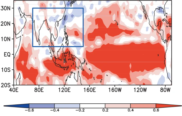
A key to seasonal prediction is to understand the relationship between the slowly varying boundary conditions and rainfall anomalies. We found that all models tend to yield positive SST-rainfall correlations in the heavily precipitating summer monsoon regions that are at odds with observations.As shown inFig. 2a (page 16), the local SST and precipitation anomalies are negatively correlated in the western North Pacific (WNP, 5o_N-30o_{N, 110-150}o_{E) and insignificantly correlated in the Bay}

of Bengal. However, the SST-rainfall correlations in the MME hindcast disagree with observations primarily in the APSM regions, where the model rainfall tends to correlate positively with local SST (Fig. 2b page 16). Over the WNP, the observed correlation is –0.36 while in the multi-model ensemble hindcast it is 0.24, both statistically significant at the 99% confidence level. The models’ inability to predict summer monsoon rainfall appears to happen because the models produce a wrong relationship between rainfall and SST in that region.

In general, a negative correlation between the seasonal-mean SST and rainfall anomalies may indicate that the atmosphere, on average, affects SST more than SST affects the atmosphere; conversely, a positive correlation means that the ocean plays a major role in determining the atmospheric response (Wang et al. 2004). To support this assertion, we further computed the lag correlations between monthly mean SST and rainfall anomalies. As shown in Fig. 3a (page 16), when precipitation leads SST by one month, there is a significant negative relation in the APSM region, suggesting that the atmosphere influences SST variability. Of note is that the simultaneously monthly correlations are also negative though in less degree. However, when SST precedes precipitation by one month, the correlations in the same region become positive. Given the persistence of SST anomalies and the rapid response of the atmosphere to SST, the negative simultaneous correlation and the weak positive lag correlation suggest that the impact of SST on the atmosphere is weak. Thus, the SST anomalies in the APSM region cannot be interpreted as a forcing; rather the SST anomalies in this region are, on an average, determined by the anomalous atmospheric conditions.

The finding that the models are unable to reproduce the observed SST-rainfall relationship provides a clue to why these models are unsuccessful in hindcasting summer monsoon rainfall. While the models’ deficiencies are somewhat to blame, we offer that the models’ failures are likely due to the lack of atmospheric feedback to the ocean, an inherent problem in the experimental design, because in the hindcast experiments the SST is prescribed as a forcing.

To test this idea, we performed a suite of numerical experiments with a coupled atmosphere-ocean model. The atmospheric component of this coupled model is the T30 version of the ECMWF-Hamburg (ECHAM4) AGCM (Roeckner et al. 1996). The ocean component is a 2-layer tropical upper-ocean model (Wang et al., 1995; Fu and Wang, 2001). The coupling, namely atmosphere-ocean interaction, was through both the momentum and heat flux exchanges without flux correction. Daily coupling was applied to the global tropics between 30o_S

and 30o_{N and climatological SSTs outside the tropics and sea}

ice were specified. The coupled model was integrated for 50 years, and the last 40 years of data were used for analysis. This

coupled model, in general, realistically simulates the climatological mean precipitation and SST, the spatial pattern and temporal characteristics of El Niño-Southern Oscillation, and the tropical intraseasonal oscillation (Fu et al. 2003). In the coupled experiment, the AGCM is allowed to interact with a tropical ocean model. For comparison a “forced” experiment was also performed in which the same AGCM was integrated using, as lower boundary forcing, the same SSTs that were produced by the coupled model. The only difference between the coupled and forced experiments is in their initial conditions, which are trivial for climate simulation and prediction. The differences in the simulation outcomes between the two experiments can be interpreted as being due to the lack of atmospheric feedback.

Figure 3b (page 16) presents the results obtained from the coupled model simulation. The simultaneous and the lag correlation patterns bear qualitative similarities with the corresponding observed counterparts, although in the coupled simulation the simultaneous negative correlations are somewhat lower and the positive correlations at lag +1 are higher. When rainfall leads SST by 1-month, the monsoon precipitation and SST are significantly negatively correlated, resembling closely the observations. In contrast, the results obtained from the forced experiment (Fig. 3c) show a significant concurrent positive correlation and similar positive, but lower, lead-lag correlations. This persistent positive correlation pattern with a concurrent maximum suggests that the slow variations of SST in the model act to regulate local rainfall anomalies. The atmospheric response to the underlying SST forcing is sufficiently rapid to cause the maximum monthly correlation to occur without a lag.

The coupled model results have been compared with the newly released multi-model seasonal prediction experimental results from the European Union-funded DEMETER project (Development of a European Multi-model Ensemble system for seasonal to interannual prediction) (Palmer et al. 2004). The coupled model forecasts for boreal summer (May to October) demonstrate that the local SST-precipitation relationships in all the models are similar to that shown in Fig. 3b, confirming that these coupled models, despite their different physical schemes, are able to produce qualitatively realistic SST-rainfall relationships. In addition, when these atmospheric models are driven by persistent SSTs the local SST-rainfall correlations become similar to those found in the forced run (Fig. 3c).

response tends to produce a positive local rainfall-SST relationship.

The present finding suggests that contrary to conventional notion, the heavy summer monsoon rainfall cannot be simulated or predicted correctly by prescribing lower boundary forcing. The coupled atmosphere-ocean processes are extremely important for seasonal prediction of monsoon rainfall. This calls for rethinking current strategies for validating dynamic climate models and for climate prediction. To adequately identify the deficiencies of models in simulating summer monsoon variability, a coupled atmosphere-ocean model is needed. The current two-tier approach predicts future atmospheric conditions using an AGCM alone forced by pre-forecast SSTs (Bengtsson et al. 1993). This strategy works for the most important forcing (Equatorial Pacific SST forced heating) and for those regions where SST determines the local wind convergence and SST itself is primarily determined by ocean processes. However, in the Asian-Pacific summer monsoon regions, where atmospheric feedback plays a major role in determining local SST, the two-tier approach would yield a forced solution that differs from realistic coupled solutions. Therefore, only coupled atmosphere-ocean models or regionally coupled models will be able to correctly forecast the predictable portion of the monsoon rainfall. Further studies of the climate predictability in the summer monsoon regions using more models and longer term integrations are needed to confirm that the present conclusions are independent of models’ physical parameterizations.

Acknowledgments

This work is in part supported by NSF Climate Dynamics program and NOAA OGP/Pacific Program. DR was supported by the EU-funded DEMETER project (EVK2-1999-00024).

References

Bengtsson, L., U. Schlese, E. Roeckner, M. Latif, T. Barnett, and N. Graham, 1993: A two-tiered approach to long-range climate forecasting. Science, 261, 1026-1029.

Charney, J. G., and J. Shukla, 1981: Predictability of monsoons.

Monsoon Dynamics, J. Lighthill and R. P. Pearce, Eds., Cambridge University Press, 99-109.

Fu, X., and B. Wang, 2001: A coupled modeling study of the seasonal cycle of the Pacific cold tongue. Part I: simulation and sensitivity experiments. J. Climate, 14, 765-779.

Fu, X., B. Wang, T. Li, and J. P. McCreary, 2003: Coupling between northward-propagating, intraseasonal oscillations and sea-surface temperature in the Indian Ocean. J. Atmos. Sci., 60, 1733-1753.

Gadgil, S., and S. Sajani, 1998: Monsoon precipitation in the AMIP runs. Climate Dyn., 14, 659-689.

Gates, W. L., and coauthors, 1999: An overview of the results of the Atmospheric Model Intercomparison Project (AMIP I). Bull. Amer. Meteor. Soc., 80, 29-56.

Palmer, T. N., and coauthors, 2004: Development of a European multi-model ensemble system for seasonal to inter-annual prediction (DEMETER).

Bull. Amer. Meteor. Soc., in press.

Reynolds, R. W., N. A. Rayner, T. M. Smith, D. C. Stokes, and W. Wang, 2002: An improved in situ and satellite SST analysis for climate. J. Climate, 15, 1609-1625.

Roeckner, E., and coauthors, 1996: The atmospheric general circulation model ECHAM-4: model description and simulation of present-day climate. Max-Planck-Institute for Meteorology, Rep.218, 90 pp.

Shukla, J., 1998: Predictability in the Midst of Chaos: A scientific basis for climate forecasting. Science, 282, 728-731. Wang, B., T. Li, and P. Chang, 1995: An intermediate model of

the tropical Pacific Ocean. J. Phys. Oceanogr., 25, 1599-1616.

Wang, B., I. S. Kang, and J. Y. Lee, 2004: Ensemble simulations of Asian-Australian monsoon variability by 11 AGCMs.

J. Climate, 17, 803-818.

Xie, P., and P. A. Arkin, 1997: Global precipitation: A 17-year monthly analysis based on gauge observation, satellite estimates, and numerical model outputs. Bull. Amer. Meteor. Soc., 78, 2539-2558

WCRP is celebrating its 25th anniversary and, as a first way to mark the event, has published a new WCRP Brochure

Abstract

A multi-model system has been used to predict the seasonal and annual sea surface temperature anomalies (SSTA) over the tropical Pacific Ocean since 1997 in the National Climate Center (China). The evaluations of the model system indicated that the ensemble multi-model predictions were better than those using by a single model.

Introduction

Many Chinese researchers have pointed out the significant correlations between the SSTA over the ENSO regions, Kuroshio and the warm pool areas of the tropical Pacific Ocean and the summer rainfall in China, as well as typhoons over the northwestern Pacific Ocean (Wang, 2001). Therefore, it is important to forecast the SSTA over the tropical Pacific Ocean.

A project on the use of a multi-model system for seasonal and annual forecasts of the SSTA over the tropical Pacific Ocean was conducted in China during the period 1996 to 2000. Several modelling groups such as the National Climate Center (NCC, China), Chinese Academy of Meteorological Sciences (CAMS), Peking University (PKU), Nanjing University (NJU), Nanjing Institute of Meteorology (NIM) and Institute of Shanghai Typhoon (STI) took part into this project (Zhao et al., 2001). Since the beginning of 1997, the multi-model system joined the National Workshops on multi-seasonal predictions in China held by the China Meteorological Administration and Hydrological Department.

In this paper, a brief description of the multi-model system and its predictions will be introduced.

Brief description of the multi-model system

There are five models in the multi-model system (Li et al., 2000; Zhao et al., 2001). They are the NCCo based on Zebiak and Cane (1987, ZC87) with improved initial conditions (Li and Zhao, 2001), NCCn based on ZC87 with improvements to some parameters in the model (Zhang and Zhao, 2000 ), CAMS/NJU based on ZC87 and developed for the global tropical Ocean (Atlantic, Indian and Pacific Oceans) (Ni et al., 2000; Shi et al., 2000), STI/NCC based on ZC87 but with assimilation of inputs as in Duan et al., 2000; Liang et al., 2000, and NIM/NCC based on the Oxford model (Balmaseda et al, 1994) with improvements to the statistical atmosphere and some parameters in the ocean model (Zhang and Ding, 2000).

In the multi-seasonal predictions by the multi-model system, each model was first run to produce an ensemble size of 5 or 6; secondly, the ensemble of the five sets of

model predictions was taken as the multi-model system’s predictions. Because the National Workshop is held in March of each year, the multi-model system predicted the period of the coming March to the following February. The system predicted the monthly SSTA over the tropical Pacific Ocean and in NINO regions (such as Nino1+2, Nino3, Nino3.4 and Nino4). The multi-model system also provided the predictions of SSTA (October ~ next September and June ~ next May) in the Annual Workshop held in October and the Special Summer Workshop of China held in June, respectively.

The seasonal and annual hindcasts and prediction of Nino3 index by the multi-model system have been evaluated for the periods of 1961~1996, 1997~2000 and 2001~2004 using anomalous correlation coefficients and standard deviations, respectively (Li et al., 2000; Zhao et al., 2000; Zhang, 2004).

Predictions

The evaluations of the seasonal and annual hindcasts of Nino3 index by the multi-model system indicated that the ensemble multi-model were better than a single model. For 1997~2004, the multi-models system predicted the weakening of El Nino events reasonably, but the starting time of El Nino events was unstable. As two examples from 2000~2004, Fig.1 and Fig.2 (page 17) give the predictions of Nino3 index for March 2001 ~ January 2002 predicted by February 2001 and for October 2003 ~ September 2004 predicted by September 2003, respectively.

Future

The multi-model system for the seasonal and annual predictions of SSTA was made up of the simplified models. The system is going to be improved in future. The predictions of SSTA by the coupled AOGCM of NCC will be combined with the system.

Acknowledgements

This research was supported by the National Key Projects and extension project of China. We sincerely thank M.Cane and S.Zebiak and National Climate Center (China) for their guidance and support.

References

Balmaseda, M. A., D. L. T. Anderson and M. K. Davey, 1994: ENSO prediction using a dynamical ocean

model coupled to statistical atmospheres. Tellus,

46A, 497-511.

Duan, Y and Liang X, 2000, Investigation of STI/NCC,

Acta Meteorologica Sinica, 870-880 (in Chinese). Seasonal and annual predictions of sea surface temperature anomalies over the tropical Pacific Ocean by using a multi-models system

Zong-Ci Zhao, Zuqiang Zhang and Qingquan Li

Li, Q, Zhao Z-c, Zhang Z, Yi L, Zhang Q, Liang X, Duan Y, Li Y, Shi L, Yin Y, Ni Y, 2000, The predictions of the 1997~1999 El Nino/La Nina events by using an intermediate ocean-atmosphere coupled model

system, Acta Meteorologica Sinica, 838-847 (in

Chinese).

Li Q and Zhao Z-c, 2001, Diagnostic analysis and verification of prediction of the tropical Pacific Sea surface temperature anomalies during 1997~1998,

J.of Tropical Meteorology, 7, 144-153.

Li, Q, 2001, Prediction of SSTA for 2001, report at National Workshop of 2001 (in Chinese).

Liang X and Duan Y, 2000, Predictions of ENSO by STI/

NCC, Acta Meteorologica Sinica, 891-897 (in

Chinese)

Ni, Y, Li S and Yonghong Y, 2000, Investigation of CAMS/ NJU, Acta Meteorologica Sinica, 848-858 (in Chinese).

Shi, L, Yongqi N and Yin Y, 2000, Experiments of SSTA

predictions over the global tropical oceans, Acta

Meteorologica Sinica, 859-869 (in Chinese).

Wang, S-W, ed, 2001, Advances on modern climatology, China Meteorological Press, Beijing, China, pp450 (in Chinese).

Zebiak,S.E. and Cane,M.A.,1987:A model of the El

Nino-Southern Oscillation. Mon.Wea.Rev.115,2262-2278.

Zhang, Q and Yihui D, 2000, Investigation on NIM/NCC model and its prediction, Acta Meteorologica Sinica, 880-890 (in Chinese).

Zhang Z and Zhao Z-c, 2000, The simplified ENSO prediction model NCCn, Short-term Climate Prediction Operation Dynamic Model, ed. By 96-908 Project, China Meteorological Press, 351-361 (in Chinese).

Zhang, Z, 2003, Annual predictions of SSTA, report at National Workshop of 2003 (in Chinese).

Zhang, Z, 2004, Perfomance of the NCC multi-models system for the prediction of SSTA, Report of NCC (in Chinese).

Zhao, Z-c, Qingquan L, Zuqiang Z, Lan Y and Zongqun Z, 2000, Relationships between ENSO and climate

change in China and predictions of ENSO, World

Resource Review (USA), 12, 2, 269-279.

Zhao Z-c, Li Q, Zhang Z, Yi L, Zhang Q, Liang X, Duan Y, Li Y, Shi L, Yin Y, Ni Y,, Qian W, Li L, and Sun Y, 2001, Advances on a dynamic prediction model system of ENSO, Short-term climate prediction dynamic model system, ed. By 96-908, China Meteorological Press, 323-335 (in Chinese).

A significant decrease of rainfall has been detected during March in the second half of the 20th century in Spain and Portugal (Trigo and DaCamara, 2000) and in the whole Mediterranean-Atlantic region (Norrant and Douguédroit, 2004). A link between Pacific atmospheric circulation indices, particularly ENSO, and springtime precipitation in Spain has been detected (Rodo et al., 1997, Knippertz et al., 2003). Our research looks for the low frequency circulation patterns of the northern hemisphere that can influence the March precipitation decrease in the Mediterranean-Atlantic region from 1951 to 2000. The relationship was studied simultaneously and with a one and two month lead time, to take into account the delay necessity for the Rossby waves to propagate from the Pacific to the western Mediterranean (Benedict et al., 2004).

1. Data and methods

Scores linked with the factor of a Rotated Principal Component Analysis (RPCA), of R type and with a Varimax rotation (Richman, 1986), on 61 stations of the Mediterranean Basin and the Atlantic coast at the same latitude from March 1951 to March 2000, form the precipitation data.

The 500hPa geopotential height data (March, February and January) come from the NCEP/NCAR reanalysis project; a

window of the northern hemisphere north of 20°N has been

retained, with a diamond grid similar to that of Barnston and Livezey (1987). The main hemispheric teleconnection indices (NCEP/NCAR) have also been used.

RPCAs, R type, have been performed on the March, February and January 500hPa geopotential heights in order to detect the main low frequency patterns of the atmospheric circulation.

2. Results

2.1. RPCA on the 500hPa geopotential height

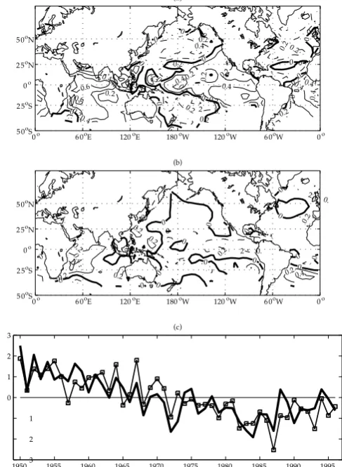
In the 12 retained factors (79,7% of the total variance) of the RPCA on the March 500hPa geopotential height, four patterns are significantly correlated with the Mediterranean-Atlantic region rainfall and explain 36% of their total variance. Two of them fit the EAtl/WRussia and NAO patterns spatial schemes (Barnston and Livezey, 1987) (Figure1, Table 1).

Among the fifteen factors retained from the RPCA on the February 500hPa geopotential height, 3 significantly correlated with the Mediterranean-Atlantic region only represent 16% of the total variance. For January they are, among a total of thirteen, 3 with 33% of explained variance (Figure 2, Table2). The strong negative correlation with the January PNA which explains on its own nearly 25% of the March rainfall in the Mediterranean-Atlantic region can be highlighted.

Predictability of the March precipitation in the Mediterraneo-Atlantic region by the PNA pattern

C. Norrant and A. Douguédroit

2.2. Correlation with the main hemispheric teleconnection indices

The correlation give the same results as the RPCA but new teleconnections with significant but weak correlation are discovered (WPac, AO) (Table 1). With a one month lead time, the single EAtl index is significantly correlated. With a two months leading time the teleconnections with the PNA index are found again. March rainfall in the Mediterranean-Atlantic region is explained at 25% by the PNA, which is the only pattern representing an important variance in the analysis.

3. Conclusion

36-40% only of the March rainfall in the Mediterranean-Atlantic region is explained by correlation with March RPCA patterns and teleconnection indices. A significant result has been obtained for their prediction with a two months lead time: PNA pattern explains 25% of their total variance. It seems to confirm the relationship previously established between Pacific and spring precipitation in western Europe by the ENSO index at a seasonal leading time (Rodo et al., 1997, Knippertz et al., 2003).

Fig.1: March patterns significantly correlated with the March rainfall of the Mediterraneo-Atlantic region. Solid line: positive correlation; dashed line: negative correlation; bold: correlation ≥0,5; contour increment: 0,1

Fig.2: January patterns significantly correlated with March rainfall of the Mediterraneo-Atlantic region. Solid line: positive correlation; dashed line: negative correlation; bold: correlation ≥0,5; contour increment: 0,1

Tab.1: Correlation of March rainfall in the Mediterraneo-Atlantic region with the main hemispheric teleconnection indices. Significant correlations are in bold.

EAtl EAtl/WRussia EPac NAO PNA Scan WPac AO SOI March -.11 .25 -.19 -.45 -.29 .13 -.23 -.34 .18

Feb -.36 .05 -.03 -.13 -.01 .13 -.03 -.19 .10

Jan -.28 -.09 -.07 .12 -.49 -.20 -.29 .06 .19

Tab. 2 Significant correlation between the scores of the March and January 500hPa geopotential height patterns and the March rainfall of the Mediterraneo-Atlantic region.

Patterns Eastern Canada EAtl / WRussia NAO Northern Siberia PNA EAtl Eurasia

March -.36 .32 -.39 .20 - -

Skill of Sahelian rainfall index in two atmospheric General Circulation model ensembles forced by prescribed sea surface temperatures

Vincent Moron

International Research Institute for Climate Prediction, Columbia University, Palisades, USA Corresponding author: [email protected]

Introduction

Sea surface temperatures (SST) changes have long been recognized as a forcing mechanism for rainfall variations in the West-African monsoon area (e.g. Rowell et al., 1995; Ward, 1998; Thiaw et al., 1999). For example, anomalous negative (positive) rainfall anomalies over the Sahelian belt (approximately between 10o _{and 20}o_{N across tropical North}

Africa) have been associated with positive (negative) SST anomalies (SSTA) throughout almost much of Indian Ocean, South and equatorial Atlantic, negative (positive) SSTA over the tropical Northern Atlantic and warm (cold) El Niño Southern Oscillation events (e.g. Rowell et al., 1995 ; Ward, 1998). SST forcing is thus potentially able to provide predictability to the Sahelian belt at seasonal time scales. Hindcast (i.e. forecast for past periods) ensembles are a standard method of estimating the uncertainty in seasonal climate prediction by sampling the distribution of possible outcomes conditional upon a given SST pattern. The potential predictability (estimated through the degree of similarity amongst an ensemble of runs that differ only by their initial conditions) and skill (estimated through the similarity between simulated and observed variability) could be based on atmospheric general circulation model (AGCM) simulation using observed SST (Sperber and Palmer, 1996). These AGCM simulations provide an indication of model performance assuming perfect SST forecasts. There are various sources of errors, decreasing the potential predictability and skill of any simulated variable such as rainfall. The chaotic evolution of the atmosphere is one major source. Over the Sahel, the percentage of SST-forced variance in seasonal rainfall amount is typically below 25-50% (10-30%) on a regional (grid-point) basis. A large part of the inter-annual variability of the seasonal rainfall is thus unpredictable from the global SST anomalies. The simulated rainfall fields could be shifted spatially relatively to observation. There are also deficiencies due to truncation and the parametrization schemes used to generate rainfall in the AGCMs. All these errors may be model- and time scale-dependent. The skill of a Sahelian rainfall index is here

investigated in two large AGCM ensembles forced by prescribed SST over the post-war II period.

Models experiments and observed data

The simulated rainfall were provided by the outputs of the ARPEGE and ECHAM 4.5 AGCMs, run respectively at the T63L30 and T42L19 resolution in a simulation mode, are used. Both ensembles (8-member for ARPEGE and 24-member for ECHAM 4.5) are forced by prescribed SST from 1948 to 1997 (ARPEGE) and from 1950 (ECHAM 4.5). These runs have been extensively presented elsewhere (Cassou and Terray, 2001; Moron et al., 2003, 2004 for ARPEGE; Tippett et al., 2004; Gong

et al., 2003 for ECHAM 4.5). The observed rainfall was obtained from the Climatic Research Unit dataset (version 1.0 ; http://

www.cru.uea.ac.uk/~mikeh/datasets/global/ ) at the 3.75o

x 2.5o _{resolution. Monthly data are available from 1901 to 1998}

but 1997 is completely missing over the Sahel. So, the data from 1950 to 1996 are used in the following analysis. In this paper, we define the Sahel as the region between 16o_W-20o_E

and 11.25o_-18.75o_{N. Time series of seasonal rainfall within the}

sahelian box are standardized to zero mean and unit variance. The standardized anomaly index (SRI hereafter) is the mean of these values (Katz and Glantz, 1986). To ease the comparison between observation and models, SRI is then re-standardized to unit varinace. Each run of both AGCMs is processed independently from each others (i.e. data are firstly standardized on a grid-point basis, then averaged into the SRI box, and SRI is thus standardized to unit variance). In the following SRI_obs, SRI_echam and SRI_arp refer respectively to observed SRI, and simulated SRI with ECHAM 4.5 and ARPEGE. Some of the correlations are computed on two different time scales, following Ward (1998). The low frequency (LF hereafter) time scale is firstly extracted from the original time series using a nine order Butterworth low-pass filter with a cut-off at 1/8 cycle-per-year (i.e. retaining only periods less than 0.125 cpy). The high frequency (HF) variability is then defined as the difference between the original time series and the LF ones.

References

Barnston AG, Livezey RE, 1987: Classification, seasonality and persistence of low frequency atmospheric circulation patterns, Monthly Weather Review, 115: 1825-1850

Benedict JJ, Lee S, Feldstein SB, 2004 : Synoptic view of the North Atlantic Oscillation, J. Atm. Sc., 61: 121-144 Knippertz P, Ulbricht U, Marques F, Corte-Real J, 2003 : Decadal

changes in the link between El Niño and springtime North Atlantic Oscillation and European-North African rainfall, Int. J. Climatol., 23: 1293-1311

Norrant C; Douguédroit A, 2004 : Monthly and daily precipitation trends in the Mediterranean (1950-2000),

Theor. Appl. Climatol., submitted

Richman MB, 1986: Rotation of principal component, J.

Climatol., 6: 293-335

Rodo X, Baert E, Comin FA, 1997 : Variations in seasonal rainfall in Southern Europe during the present century : relationships with the North Atlantic Oscillation and El Niño – Southern Oscilation, Climate Dynamics, 13 : 275-285

Trigo RM, DaCamara CC, 2000: Circulation weather types and their influence on the precipitation regime in Portugal,

From Hazeleger, Page 7: Report on Tropical Atlantic Workshop

Figure 1: Scheme showing proposed observtions during the 1-5 year enhanced observation period of CLIVAR-TACE (courtesy of W. John, RSMAS)

From Wang et al Page 8: Challenges in Prediction of Summer Monsoon Rainfall: Inadequacy of the two-tier strategy.

From Wang et al Page 8: Challenges in Prediction of Summer Monsoon Rainfall: Inadequacy of the two-tier strategy.

Fig. 2. (a) Observed and (b) simulated correlation coefficients between the June-August SST and precipitation anomalies (the color shadings). The contours denote the climatological June-August mean rainfall rate (in units of mm day-1_{) that highlight the}

regions of heavy precipitation. The observed correlations were computed using 20 years of data (1982-2001) derived from CMAP rainfall (Xie and Arkin 1997) and Reynolds (Reynolds et al. 2002) SST. The simulated results were made by 5 AGCM’s multi-model ensemble hindcast.

From Zhao et al, Page 11: Seasonal and annual predictions of sea surface temperature anomalies over the tropical Pacific Ocean by using a multi-models system

Fig.1 Multi-seasonal predictions of Nino3 index for March 2001 ~ January 2002 (Li, 2001)

Fig.2 Multi-seasonal predictions of Nino3 index for October 2003 ~ September 2004 (Zhang, 2003)

Figure 1 - Rainfall rate (mm/day; shaded) and SST (ºC; contour) for (a) CTRK, (b)

CK, (c) WK,(d) CRTA,(e) CA and (f) WA

experiments.

From Chaves and Ambrizzi, page 24: Atmospheric response for two convection schemes in sensitivity experiments using SST anomalies over the South Atlantic Ocean

Fig. 2. Logarithm of the (negative) vertical integral of the passive salinity anomaly tracer in the EBM experiment. The tracer shows the direct effect of the fresh water flux anomaly around the coasts of Greenland. The figure shows the average over the last twenty years (80-100) of the experiment.

Figure 1. Elevation (mm) for tropical South America. The box (10º-22ºS, 42º-55ºW) includes the headwater regions for major rivers flowing into the 1) Tocantins, 2) São Francisco, and 3) Paraná/ La Plata basins. The numbers on the map indicate the locations of the following water reservoirs: 1) Sobradinho, 2) Três Marias, 3) Emborcação, 4) Itumbiara, 5) Furnas, and 6) Jurumim.

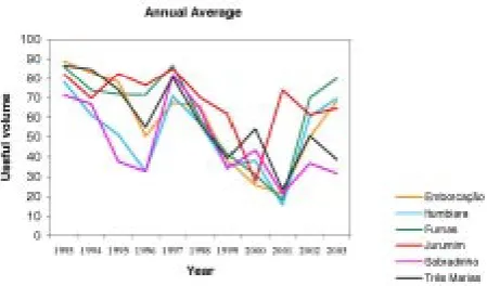
Figure 2. The mean annual cycle of precipitation (mm) for central Brazil (10º-22ºS, 42º-55ºW), as indicated in Fig. 1, and the mean annual cycle for the useful water volume (%) for the six reservoirs. The useful volume is the water volume between the maximum and minimum levels for which the dam can produce electricity From Silva et al, Page 23: CLIVAR Science: application to energy: The 2001 energy crisis in Brazil

Figure 3. Useful volume annual average (%) from 1993 to 2003 for reservoirs indicated in Fig. 1. The useful volume is the water volume between the maximum and minimum levels for which the dam can produce electricity.

Figure 4. Mean anomalous precipitation for October-April 1995/96 to 2000/01. Data are derived from the daily gridded analyses of precipitation produced by the NOAA/ Climate Prediction Center

Raw and adjusted skill of ECHAM 4.5 and ARPEGE

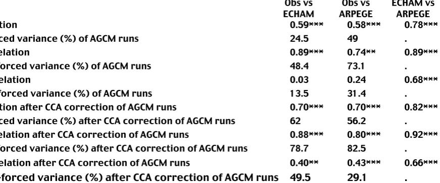
Figure 1 displays the one–point correlation between SRI_obs and the observed gridded rainfall (Figure 1a), then with ARPEGE (Figure 1b) and ECHAM 4.5 (Figure 1c) simulated rainfall. Concerning observations (Figure 1a), the zonal consistency of the Sahelian rainfall variability is striking with correlations over 0.5-0.6 stretched eastward outside the SRI box, to the Red Sea. Note also large positive correlations over Guinean mountains and also over the Southern Chad and the Sudan (Figure 1a). The correlations between SRI_obs and ARPEGE rainfall (Figure 1b) match the observed pattern quite well, with a slight northward shift. The correlations are also weaker over the western part of the SRI box (Figure 1b). The maximum in the correlations between SRI_obs and ECHAM 4.5 simulation (Figure 1c) are slightly southward shifted over central Sahel, with a large northeastward extension of positive correlations over the eastern Sahara (Figure 1c). Even if the correlations inside the SRI box are significant, slight shifts of the pattern occur for both AGCMs. When the same boundary limits as in observation are considered, the correlations between SRI_obs and simulated SRI are significant at the 0.01 one-sided level, but the skill is largely due to decadal variability and trends (Table 1). At high-frequency time scales (Table 1), the correlations are not significantly different from zero for both AGCMs. Both AGCMs remain significantly correlated with each other on LF but also on HF time scale (Table 1), suggesting that the SST-forced component is quite robust and almost unconditional upon the AGCM used.

The spatial shift of the teleconnection observed in Figure 1b and 1c, could be easily corrected by a linear method such as Canonical Correlation Analysis (CCA). Model outputs are adjusted based on the leading two CCA modes between the large-scale (i.e. concatenated runs on 50o_W-50o_{E and 0}o_-35o_N)

simulated rainfall and the regional-scale observed rainfall inside the SRI box (Ward and Navarra, 1997 ; Moron et al., 2001). To avoid overfitting, 5 years from 1950 to 1996 are held out in turn and CCA is used to develop a prediction model using the remaining 42 years. The temporal correlation

between the CCA cross-validated hindcasts and SRI_obs is

improved, mainly at HF time scale (Table 1). In the following, SRI_arp and SRI_echam refer to simulated rainfall obtained from the CCA cross-validated hindcasts.

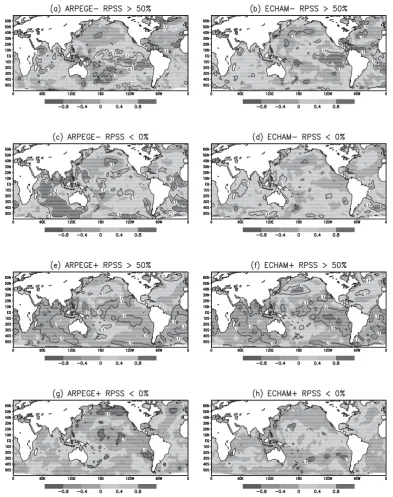
The skill for each year is evaluated using the Rank Probability Skill Score –RPSS hereafter-(Doblas-Reyes et al., 2000). Rank Probability Score (RPS, Epstein, 1969) is here defined with terciles (SRI_obs time series is divided into three categories having respectively 16,15 and 16 members and SRI_arp and SRI_echam are ranked into these categories). RPS is referred to climatology to give RPSS, which represents a percentage improvement in RPS over the 1950-1996 climatology. A RPSS of 100% means that all runs are in the same class as the observed value. A negative RPSS indicates skill worse than climatology. RPSS is below zero in 1960, 1973, 1976, 1981, 1985, 1988, 1993, 1994 and 1995 for both AGCMs, 1970, 1979, 1987, 1990 for ARPEGE only and 1951, 1965, 1966, 1969, 1977, 1978, 1996 for ECHAM only (Figure 2). It seems that the unskillful years are thus concentrated during the dry period, from 1968. On the contrary, the most

skillful years, having a RPSS over 50%, occur mostly during the wet period, till 1967 (Figure 2).

The origin of errors could be various. First of all, it is known that the observed network deteriorates from the 1970s. Fewer stations could decrease the signal-to-noise ratio of the regional index and thus make it less predictable. The CPC merged analysis of precipitation (CMAP) dataset, from gauge data and satellite estimates, could be used as an alternative of the surface CRU dataset. The data are available from 1979 on a 2.5 x 2.5 grid. The SRI computed from the CMAP dataset is correlated at 0.93*** (in the following, one, two and three stars indicate significant correlations at the one-sided 0.1, 0.05, 0.01 levels according to a random-phase test (Janicot et al., 1996) with 10000 random time series) with SRI_obs on the 1979-1996 period and no systematic increase of the difference between both indices is observed (not shown), suggesting that the decrease of the skill of the AGCMs may not be related to the deterioration in the observed network. Of course, these errors could be due to sampling variations but the apparent concentration of the unskillful years during the dry period for both AGCMs is intriguing. Firstly, the AGCM could be wrong in the transmission of a particular SST forcing onto the atmosphere,

Figure 1 : correlation (x 100) maps between SRI_obs and (a) observed JAS seasonal rainfall (from CRU dataset) ; (b) simulated JAS seasonal rainfall (mean ensemble from ARPEGE) ; (c) simulated JAS seasonal rainfall (mean ensemble from ECHAM 4.5). In panels (b) and (c), contours are traced at 30, 40, 50 and 60 only. The SRI box is contoured on each map

Continued from page 14

(a)

5 22 24 223 15 26 19 4 2 4 1 116 16 22 28 3115 27 25 10 27 34 3 5 2 1 0 6 6 15 33 15 9 52 19 2 28 35 24 311 3 7 5 6 4 5 4 5 2 0 4 7 2 8 24 72 76 51 29 11 34 15 26 66 72 52 59 55 41 45 68 38 82 77 85 83 79 83 83 84 83 71 82 78 71 70 51 49 43 69 83 82 82 83 91 89 78 65 78 76 75 53 34 20 9 4 4 2 567 78 71 78 835 3 75 51 38 59 563 68 190 5 0 5 0

11 23 41 16

10 13 0 0 0 1 3

25 17 1715 1 7 14 0 0

2 3 8 5 15 12 9 8 2 105 17 11 7 25 37 7 16 28 32 13 7 5 2 5 4 219 6 7 10 1

1 7 12 112 1 6 6 13 0 7 1 6

1 5oW 0o 1 5oE 3 0oE 4 5oE 0o

8oN 1 6oN 2 4oN 3 2oN

(b) 30 30 30 30 30 30 30 30 30 30 30 30 30 40 40 40 40 40 40 40 40 40 50 50 50 50 50 60 60 60 60

4 0oW 2 0oW 0o 2 0oE 4 0oE 0o

6oN 1 2oN 1 8oN 2 4oN 3 0oN

(c) 30 30 30 30 30 30 30 30 30 30 30 30 30 40 40 40 40 40 40 40 40 40 40 40 50 50 50 50 50 50 50 50 50 60 60 60 60 60

4 0oW 2 0oW 0o 2 0oE 4 0oE 0o

6o_N

1 2oN 1 8o_N