An agenda based framework for multi issues negotiation

An agenda-based framework

for multi-issue negotiation

Shaheen S. Fatima

_{, Michael Wooldridge}

_{, Nicholas R. Jennings}

b_{Department of Electronics and Computer Science, University of Southampton, Southampton SO17 1BJ, UK}

Received 28 April 2002; received in revised form 28 March 2003

Abstract

This paper presents a new model for multi-issue negotiation under time constraints in an incomplete information setting. The issues to be bargained over can be associated with a single good/service or multiple goods/services. In our agenda-based model, the order in which issues are bargained over and agreements are reached is determined endogenously, as part of the bargaining equilibrium. In this context we determine the conditions under which agents have similar preferences over the implementation scheme and the conditions under which they have conflicting preferences. Our analysis shows the existence of equilibrium even when both players have uncertain information about each other, and each agent’s information is its private knowledge. We also study the properties of the equilibrium solution and determine conditions under which it is unique, symmetric, and Pareto-optimal.

2003 Elsevier B.V. All rights reserved.

Keywords: Multi-issue negotiation; Game theory; Agendas; Intelligent agents

1. Introduction

Negotiation is a means for agents to communicate and compromise to reach mutually beneficial agreements [11,14,18,29,30,40]. In such situations, agents have a common interest to cooperate, but have conflicting interests over exactly how to cooperate. Put differently, agents can mutually benefit from reaching agreement on an outcome from a

*_{Corresponding author.}

E-mail addresses: [email protected] (S.S. Fatima), [email protected] (M. Wooldridge), [email protected] (N.R. Jennings).

set of possible outcomes, but have conflicting interests over the set of outcomes. In this context, the main problem that confronts agents is to decide how to cooperate—before they actually enact the cooperation and obtain the associated benefits. On the one hand, each agent would like to reach some agreement rather than disagree and not reach any agreement. But, on the other hand, each agent would like to reach an agreement that is as favourable to it as possible.

To this end, a number of negotiation models that address this problem have been developed and applied to data allocation in information servers, resource allocation and task distribution [18,19,27,31,32]. Apart from these, another application area in which agent-mediated negotiation has received considerable attention is in the field of electronic commerce [22–24,35,36]. In this domain, which is the main focus of this paper, the aim is to build software agents that will optimally negotiate with other agents on behalf of users for buying and selling goods/services. Here we look at one-to-one negotiation between a buyer and a seller. In order to develop software agents for such bilateral encounters, we first examine the important features of real-life bargaining situations that need to be incorporated in the software agents. To this end, the three crucial features of most practical bargaining processes are as follows [28]:

(1) The time constraints of the bargainers. (2) The information state of the bargainers. (3) The number of issues to be bargained over.

We first explain the role of time in negotiation. Consider an e-commerce scenario in which a buyer agent and a seller agent negotiate over the price of a good or service. The buyer clearly prefers a low price, while the seller prefers a high one (hence the competitive nature of the encounter). In addition to attempting to obtain the best price, agents also usually need to ensure that negotiation ends before a certain deadline. However, the end point may not be the only way in which time influences negotiation behaviour. Consider the case in which the service is provided immediately after negotiation ends successfully (say at priceP and timeT). In some situations, it is not sufficient merely for an agent to ensure thatT is any time less than its deadline. This may be the case, for instance, because one of the agents, say the buyer, could be losing utility with time as a result of not getting the service. On the other hand, the seller may perhaps gain more utility by providing the service as late as possible. Thus, in this case, the seller tries to maximizeT (within the limit of its deadline) and the buyer tries to minimizeT. In short, it is clear that agents can have different attitudes toward time. Generally speaking, the most common time effects in bargaining situations are time discounting and deadlines [10,21]. An agent that gains utility with time and has the incentive to reach a late agreement (within its deadline) is said to be a strong or patient player. An agent that loses utility with time and tries to reach an early agreement is said to be a weak or impatient player. As we will show, this disposition and the actual deadline itself strongly influence the negotiation outcome.

which affect the ability of an individual to make choices in a given situation. For instance, in bargaining between a buyer and a seller, information includes not only information about an agent’s own parameters (such as its reservation price or its preferences over possible outcomes), but also those of its opponent. In most realistic cases agents have only incomplete information about their opponent.

To this end, game theoretic models have already been proposed for bargaining with incomplete information. For instance, Rubinstein [34] developed a model in which agents have incomplete information about time preferences. Fudenberg et al. [12] analyse buyer-seller negotiation in which reservation prices are uncertain. Sandholm and Vulkan [37] consider uncertainty over agent deadlines. All these models are built on the assumption that information about the uncertain parameter (in the form of possible values and a probability distribution over them) is the agents’ common knowledge. However, in practice, perhaps the main way of acquiring information about the opponent is through learning from previous encounters. In such cases, an agent’s beliefs about its opponent will not be known to its opponent. We therefore study the strategic behaviour of agents by treating each agent’s information as its private knowledge.

The third key feature is the number of issues that have to be negotiated. In many of the applications that are conceived in the domain of e-commerce, it is important that the agents should not only bargain over the price of a product, but also take into account issues such as the delivery time, quality, payment methods, and other product specific properties. In such multi-issue negotiations, one approach is to bundle all the issues and discuss them simultaneously as a complete package. This allows the players to exploit trade-offs among different issues, but requires complex computations to be carried out [4,17]. The other approach, which is computationally simpler, is to negotiate the issues sequentially. A second and more important reason why parties may choose to settle issues one by one is the strategic implications of the choice of the negotiation procedure (i.e., issue-by-issue vs. complete package). When there are two objects to negotiate, the decision to negotiate them simultaneously or one by one is by no means neutral to the outcome [2,38]. Although issue-by-issue negotiation minimizes the complexity of the negotiation procedure, an important question that arises is the order in which the issues are bargained over. This ordering is called the negotiation agenda and it has been shown to be one of the factors that determines the outcome of negotiation [9]. For instance, if there are two issues,

X andY, the two agendasXY andY X can lead to two different outcomes. The agents need not have identical preferences over these outcomes and one of them may prefer the agendaXY toY X, while the other may preferY XtoXY. Given this fact, exploring the role of the bargaining agenda, and how players might manipulate it, is timely, especially given that many real-life negotiations involve multiple issues.

There are two ways of incorporating agendas in the negotiation model. One is to fix the agenda exogenously as part of the negotiation procedure. Considering the above example, one of the agendas, say XY is imposed exogenously. Then the bargainers have to settle

Existing game theoretic models for issue-by-issue negotiation [1,9,16], which are basically extensions of [33,34], have two main shortcomings. Firstly, they study the strategic behaviour of agents by treating the information they have as common knowledge. In practice however, the information that a player has about its opponent is mostly acquired through learning from previous encounters. An agent’s beliefs about its opponent will therefore not be known to its opponent. Secondly, these models do not consider agent deadlines. We overcome these problems by considering each agent to have its own deadline and by treating each agent’s information state as its private knowledge. In this case we obtain the connection between this private knowledge and the existence of equilibrium for single issue negotiation. We then extend this model for multi-issue negotiation and study the properties of the equilibrium solution.

To provide a setting for our negotiation model, we consider the case in which negotiation needs to be completed by a specified time, which may be different for different parties (since this is the most realistic case). Apart from the agents’ respective deadlines, the time at which agreement is reached can affect the agents (patient or impatient) in different ways [7]. To this end, Fatima et al. [7] presented a single-issue model for negotiation between two agents under time constraints and in an incomplete information setting by considering the agents’ information as its private knowledge. Within this context, they determined optimal strategies for agents but did not address the issue of the existence of equilibrium. Here we adopt this framework and prove that mutual strategic behavior of agents, where both use their respective optimal strategies, results in equilibrium. We then extend this framework for multi-issue negotiation. The order in which issues are bargained over and agreements are reached is determined by the equilibrium strategies. The time of equilibrium agreement may not be equal for all the issues. Consequently, the outcome of multi-issue negotiation can be implemented in two ways: sequentially or simultaneously. We then determine conditions under which agents have similar, as well as conflicting, preferences over the implementation scheme. Finally, we study the properties of the equilibrium solution.

This work extends the state of the art in multi-issue negotiation by presenting a more realistic negotiation model that captures the three aspects, mentioned above, that are associated with many real-life bargaining situations. Firstly, it is a model for negotiating multiple issues. Secondly, it takes the time constraints of bargainers into consideration, both in the form of agent deadlines and their discounting factors. Thirdly, it allows agents to have incomplete information about each other, and each agent’s information is treated as its private knowledge. Although we study bargaining in which agents have one specific information state and the agenda is endogenous, our negotiation framework is general and can be used for exploring a wide range of negotiation environments by changing the agents’ information states or the way in which the players manipulate the agenda.

2. Components of a negotiation model

The four components of a negotiation model are as follows [31]:

(1) The negotiation protocol. (2) The negotiation strategies. (3) The information state of agents. (4) The negotiation equilibrium.

The protocol specifies the rules of encounter between the negotiation participants. That is, it defines the circumstances under which the interaction between agents takes place, what deals can be made and what sequences of offers are allowed. In general, agents must reach agreement on the negotiation protocol to use before negotiation proper begins. A negotiation protocol can be designed for handling a single issue or multiple issues. Within the class of multi-issue negotiations, we can have protocols that negotiate on all the issues together or one by one.

An agent’s negotiation strategy is a specification of the sequence of actions (usually offers or responses) the agent plans to make during negotiation. There will usually be many strategies that are compatible with a particular protocol, each of which may produce a different outcome. For example, an agent could concede in the first round or bargain very hard throughout negotiation until its timeout is reached. It follows that the negotiation strategy that an agent employs is crucial with respect to the outcome of negotiation. It should also be clear that the strategies which perform well with certain protocols will not necessarily do so with others. The choice of a strategy to use is thus a function not just of the specifics of the negotiation scenario, but also the protocol in use.

An agent’s information state describes the information it has about the negotiation game. Von Neumann and Morgenstern [26] introduced the fundamental classification of games into those of complete information and those of incomplete information. The former category is basic. In these games the players are assumed to know all relevant information about the rules of the game and players’ preferences that are represented by utility functions. In the latter category, information may be lacking about a variety of factors in the bargaining problem. Thus each player may have some private information about his own situation that is unavailable to the other players, while having only probabilistic information about the private information of other players. Following Harsanyi [14,15], models of games of incomplete information proceed from the assumption that all players start with the same probability distribution on this private information and that these priors are common knowledge. This is modelled by having the game begin with a probability distribution, known to all players. Thus players not only have priors over other players’ private information, they also know what priors the other players have over their own private information. Strategic models of incomplete information thus include an extra level of detail, since they specify not only the actions and information available to the other players in the course of the game, but also their probability distributions and information prior to the start of the game.

a strategy profile must constitute an equilibrium), the earliest concept of which was the Nash equilibrium for games of simultaneous offers [25]. Two strategies are in Nash equi-librium if each agent’s strategy is a best response to its opponent’s strategy. This is a neces-sary condition for system stability where both agents act strategically. For sequential offer protocols, the Nash equilibrium concept was strengthened in several ways by requiring that the strategies stay in equilibrium at every step of the game [39]. In summary, ratio-nality, as understood in game theory, requires that each agent will select an equilibrium strategy when choosing independently. Given this, game theory prescribes the following main criteria [28] for evaluating the equilibrium outcome:

(1) Uniqueness. If the solution of the negotiation game is unique, then it can be identified unequivocally.

(2) Efficiency. An agreement is efficient if there is no wasted utility (i.e., the agreement satisfies Pareto-optimality). An outcome is Pareto-efficient if there is no other outcome that improves the payoff of one agent without making another agent worse off. All other things being equal, Pareto-efficient solutions are preferred over those that are not.

(3) Symmetry. A bargaining mechanism is said to be symmetric if it does not treat the players differently on the basis of inappropriate criteria. Exactly what constitutes inappropriate criteria depends on the specific domain. For example, if the bargaining outcome remains the same irrespective of which player starts the process of bargaining, then it is said to be symmetric with respect to the identity of the first player.

(4) Distribution. This property relates to the issue of how the gains from trade are split between the players; does the outcome split the gains equally between the traders or does it favour one agent more than the other? In this paper, our aim is not to design a negotiation mechanism that divides the gains fairly among players but to study the outcome that results when both agents are self-interested.

With these broad guidelines in mind, many different models can be designed. Below, we report on the development of a new model based on negotiation decision functions (see Section 3.2) for bargaining over multiple issues. We first describe the single issue model and study its equilibrium strategies and outcomes. We then extend this model for multi-issue negotiation and study its equilibrium properties.

3. The single-issue negotiation model

We first describe the single issue negotiation protocol and obtain the agents’ optimal strategies. We then prove that the optimal strategy profiles form sequential equilibrium.

3.1. The negotiation protocol

acceptable to both b ands (i.e., the zone of agreement) is the interval [RPs,RPb] and (RPb−RPs) is known as the price-surplus. The buyer’s initial price, IPb, has a value less than the seller’s reservation price. Similarly, the seller’s initial price has a value greater than the buyer’s reservation price. In other words, both IPband IPs lie outside the zone of agreement.

The agents alternately propose offers at times in T = {0,1, . . .}. Each agent has a deadline.Tadenotes agenta’s deadline whereTa∈T. Letpt_b→s denote the price offered by agent b at time t. Negotiation starts when the first offer is made by an agent. The agent who makes the initial offer is selected randomly at the beginning of negotiation. When an agent, say s, receives an offer from agent b at timet, i.e., pt_b→s, it rates the offer using its utility functionUs. If the value of Us forpt_b→s at timet is greater than the value of the counter-offer agent s is ready to send in the next time period,t , i.e.,

Us(p_bt_→s, t)Us(pt_s→b, t)fort =t+1, then agents accepts the offer at timet and negotiation ends successfully in an agreement. Otherwise a counter-offer is made in the next time period,t . Thus the action,As, that agents takes at timet, in response to the offerp_bt_→s, is defined as:

Ast, pt_b→s=

  

Quit ift > Ts,

Accept ifUs(p_bt_→s)Us(pt_s→b), Offerpt_s→batt otherwise.

Agents’ utilities are defined with the following two von Neumann–Morgenstern utility functions [17] that incorporate the effect of time discounting

Ua(p, t)=U_pa(p)U_ta(t). (1)

U_pa andU_ta are unidimensional utility functions. Here, preferences for attributep, given the other attributet, do not depend on the level oft.U_pais defined as:

Ua(p)=

RPb−p for the buyer,

p−RPs for the seller.

U_tais defined asU_ta(t)=(δa)t, whereδais the discounting factor. Thus when(δa>1)the agent is patient and gains utility with time and when(δa<1)the agent is impatient and loses utility with time. The utility from conflict is lower than the utility from any of the possible agreements for both agents. Each agent prefers to reach an agreement, rather than disagree and not reach any agreement at all, since the utility from an agreement is always higher than conflict utility. Consequently, it is optimal for agentato offer RPaat the latest by its deadline, if it has not done so earlier, and avoid a conflict (see Section 3.5 for details on an agent’s optimal strategy). Agents are said to have similar time preferences if both gain on time or both lose on time. Otherwise they have conflicting time preferences.

3.2. Counter-offer generation

price depending on t andTa. The initial offer is a point in the interval [IPa, RPa]. The constant ka multiplied by the size of interval determines the price to be offered in the first proposal by agenta. The offer made by agenta to agentaˆ at timet (0tTa) is modelled as a functionφadepending on time as follows:

p_at_→ˆa=

IPa+φa(t)(RPa−IPa) fora=b,

RPa+(1−φa(t))(IPa−RPa) fora=s.

A wide range of time-dependent functions can be defined by varying the way in which

φa(t)is computed (see [3] for more details). However, functions must ensure that 0

φa(t)1,φa(0)=ka (whereka lies in the interval[0,1]), andφa(Ta)=1. That is, the offer will always be between the range[IPa,RPa], at the beginning it will give the initial constant and when the deadline is reached it will offer the reservation value. The initial offer is IPa ifka=0, lies between IPa and RPafor 0< ka<1, and is RPa forka=1. Thus by varyingkabetween 0 and 1, the initial price that is offered can be varied between

IPaand RPa. Since we want IPato be the initial offer, we setka _{to 0. Functionφ}a_(t)is called the negotiation decision function (NDF) and is defined as follows:

φa(t)=ka+1−ka t Ta

1/ψ

. (2)

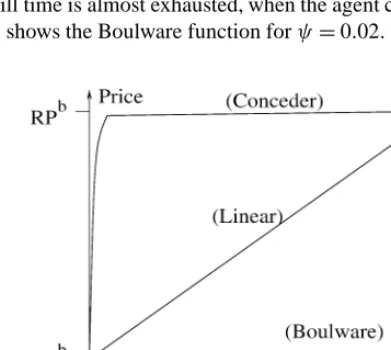
These NDFs represent an infinite number of possible tactics, one for each value ofψ(see [3] for more details). However, depending on the value of ψ, three extreme sets show clearly different patterns of behaviour (see Fig. 1).

(1) Boulware (B) [30]. For this tactic, ψ <1 and close to zero. The initial offer is maintained till time is almost exhausted, when the agent concedes up to its reservation value. Fig. 1 shows the Boulware function forψ=0.02.

(2) Conceder (C) [29]. For this tactic,ψ >1. The agent goes to its reservation value very quickly1 and maintains the same offer till the deadline. Fig. 1 shows the Conceder function forψ=50.

(3) Linear (L) Finally, whenψ=1, price is increased linearly.

The value of a counter offer depends on the initial price (IP) at which the agent starts negotiation, the final price (FP) beyond which the agent does not concede, the timet at which it offers the final price, andψ. These four variables form an agent’s strategy.

Definition 1. An agent’s strategy Sa is defined as a quadruple whose elements are the initial price(IPa)at which the agent starts negotiation, the final price(FPa)beyond which the agent does not concede, time (ta) at which the final price is offered, andψa. Thus

Sa= IPa,FPa, ta, ψa.

Agentauses its strategy,Sa, to generate an offer,pt

a→ˆa, fortt

a_{. Different strategies}

can be defined for different values of these four elements. For example, when b starts making offers ats’s reservation price, and offers its own reservation price at a time, say

T, and uses an extreme Boulware NDF, thenSbis defined asSb= RPs,RPb, T , B. Note that theB inSbis a value forψ that gives the Boulware function. In general, we useB,

C, andLto indicate a value forψthat gives the Boulware, Conceder, and Linear NDFs respectively. When both agents use strategies of this form, negotiation can end either in an agreement or a conflict, depending on the four elements that constitute each agent’s strategy.

Definition 2. The negotiation outcome (O)is an element of (p, t),C. The pair(p, t)

denotes the price and time of agreement wherep∈ [RPs,RPb]andt∈ [0,min(Tb, Ts)].

C denotes the conflict outcome.

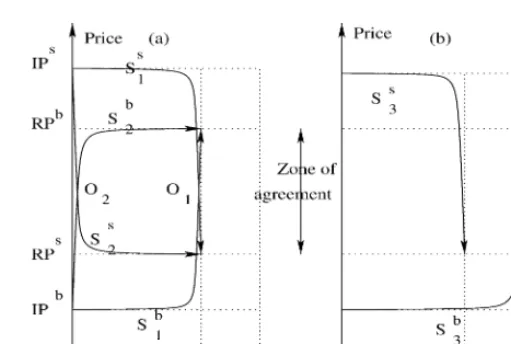
As an illustration, when agent b’s strategy is defined as S₁b= IPb,RPb, Ts, B and agents’s strategy is defined as S₁s = IPs,RPs, Ts, B, the outcome (O1) that results is

shown in Fig. 2(a) (i.e., the point where S₁b andS₁s converge). As shown in the figure, agreement is reached at a price RPs+(price-surplus/2)and at a time close toTs. Similarly when the NDF in both strategies is replaced with C, then agreement (O2) is reached at

the same price but towards the beginning of negotiation. If the agents’ strategies do not converge before the deadline, then negotiation results in a conflict. This is illustrated in Fig. 2(b), where both agents use the extreme Boulware NDF, but offer the final price at different times, thereby resulting in conflict.

Since agents are assumed to be Von Neumann and Morgenstern [26] expected utility maximizers, we need to determine the four elements of each agent’s strategy that will give

Fig. 2. Negotiation outcome for Boulware and Conceder functions. (a) Agreement. (b) Conflict.

it maximum possible utility. An agent’s optimal strategy depends on the information it has about the negotiation parameters. We therefore define the information state for each agent and then show how the optimal strategies are determined.

3.3. Agents’ information states

Each agent has a reservation limit, a deadline, a utility function and a strategy. Thus the buyer and seller each have four parameters denoted RPb, Tb, Ub, Sb and RPs, Ts, Us, Ss respectively. The outcome of negotiation depends on all these eight parameters. The information state, Ia, of an agenta is the information it has about the negotiation parameters. An agent’s own parameters are known to it, but the information it has about the opponent is not complete. We defineIbandIs as:

Ib= RPb, Tb, Ub, Sb, Ls_p, Ls_t

and

Is= RPs, Ts, Us, Ss, Lb_p, Lb_t,

where RPb,Tb_,Ub_andSb_{are the information about the buyer’s own parameters andL}s p andLs_t are its beliefs about the seller. Similarly, RPs,Ts,Us andSs are the seller’s own parameters andLb_pandLb_t are its beliefs about the buyer.Ls_t andLs_p are two probability distributions2that denote agentb’s beliefs about agents’s deadline and reservation price.

Ls_t is ann-tuple of ordered pairs of the formT_is, αs_i, where 1in. The first element in a pair,T_is, (whereT_is∈T for 1in) denotes a possible value for the seller’s deadline and the second element,α_is, denotes the probability with which the seller’s deadline isT_is.

In other words, the pairs are possible time values for agents’s deadline and the associated probabilities. One of the n possible values is agent s’s actual deadline. The pairs are assumed to be arranged in ascending order of time values, i.e.,T_is< T_is₊₁for 1in−1.

Ls_pis analogous toLs_t and denotes the buyer’s beliefs about the seller’s reservation price. The elements ofLs_p are pairs are denotedRPs_i, β_iswhere 1im. The first element is a possible value for the seller’s reservation price and β_is is the associated probability. SimilarlyLb_t andLb_pare two probability distributions that denote the seller’s beliefs about the buyer’s deadline and reservation price. The elements ofLb_t are of the formT_ib, αb_i

(whereT_ib∈T for 1in) and the elements ofLb_pare of the formRPb_i, β_ib. For our present analysis we consider the case where RPs₁<RPb_m, i.e., the highest possible value for the seller’s reservation price is less than the lowest possible value for the buyer’s reservation price.3_{We treat the agents’ beliefs as being static}4_{and not changing during negotiation.}

Thus agents have uncertain information about each other’s deadline and reservation value. Moreover, agents do not know their opponent’s utility function or strategy. In other words, an agent’s information state models two5 parameters of the opponent: the opponent’s reservation price and its deadline. Each agent’s information state is its private information that is not known to its opponent.

3.4. Negotiation scenarios

On the basis of the relationship between agent deadlines and their discounting factors, we define six negotiation scenarios. An agent negotiates in one of these six scenarios. The buyer believes that with probabilityαs_i, the seller’s deadline isT_is. This gives rise to three relations between agent deadlines. All the npossible seller deadlines could be less than the buyer’s deadline, some of them could be less and the others greater, and finally all of them could be greater than the buyer’s deadline. For each of the two possible realizations of the buyer’s discounting factor, these three relations can hold between agent deadlines. In other words, negotiation can take place in any one of the six scenarios,N1, . . . , N6, listed

in Table 1. The set of negotiation scenarios for the seller can be defined in the same way. The scenario combinations that are possible for the two agents to interact are listed in Table 2. For instance, when agentbis in scenarioN1,Tsis less thanTb. In such a situation,

agentscan only be in one of the four scenariosN2,N3,N5 orN6, sinceTs can be less

thenTbin only these four scenarios. Recall that one of the possible values is the opponent’s actual deadline. This implies that when agentbis in scenarioN1, agentscan neither be in

scenarioN1nor inN4. Thus in general when agentais in scenarioN1, agentaˆmay be in

any one of the four scenarios—N2,N3,N5, orN6. The remaining scenario combinations,

listed in Table 2 can be obtained using similar reasoning. Note that it is possible for the agents to have equal deadlines in the following cases: when both agents are in scenarioN2,

3_{Future work will deal with the situation where RP}s 1>RPbm.

Table 1

Possible negotiation scenarios for agentb

Negotiation scenario Relationship between agent deadlines Discounting factor

N1 Tns< Tb δb>1

N2 T_ks< TbT_ks₊₁ fork+1< n δb>1

N3 Tb< T1s δb>1

N4 Tns< Tb δb<1

N5 Tks< TbTks+1 fork+1< n δb<1

N6 Tb< T1s δb<1

Table 2

Possible negotiation scenarios for buyer-seller interactions

Agenta Agentaˆ

N1 N2,N3,N5,N6

N2 N1,N2,N3,N4,N5,N6

N3 N1,N2,N4,N5

N4 N2,N3,N5,N6

N5 N1,N2,N3,N4,N5,N6

N6 N1,N2,N4,N5

or when both agents are in scenarioN5, or when agentais in scenarioN2and agentaˆis

in scenarioN5. For all the other combinations, the agents have different deadlines.

3.5. Optimal strategies

We describe how optimal strategies are obtained for players that are von Neumann– Morgenstern expected utility maximizers. The discussion is from the perspective of the buyer (although the same analysis can be taken from the perspective of the seller). In order to simplify the discussion we first assume thatLs_p contains a single element, which is the seller’s reservation price, and obtain the optimal strategy. We then extend the analysis to the more general case whereLs_pcontainsmelements.

Each agent’s optimal strategy is determined on the basis of its own information state, i.e., the buyer’s optimal strategy is determined on the basis ofIband the seller’s optimal strategy is determined on the basis of Is. We then determine if this mutual strategic behavior of agents results in equilibrium.

3.5.1. Optimal strategies for the buyer whenLs_pcontains a single element

In all the six scenarios, the strategies should ensure agreement by the earlier deadline (i.e.,TsifTs< TbandTbifTb< Ts). Otherwise the agent with the earlier deadline quits and negotiation ends in a conflict, a situation which both agents prefer to avoid. We begin with scenarioN1where all thenpossible values for the seller’s deadline are less thanTb.

Since δb>1 in scenario N1, the buyer prefers to reach agreement at the latest possible

time and at the lowest possible price. AsTs < Tbin scenarioN1, the latest possible time

Fig. 3. Buyer strategies in different scenarios whenLspcontains a single element.

The outcome of negotiation depends on both agents’ strategies. Since both agents use a time-dependent strategy, an agent always plays a strategy that offers its own reservation price at its deadline. The buyer does not know the seller’s deadline, but it has a lottery

(Ls_t)overnpossible values for the seller’s deadline. So the buyer knows that if the seller’s deadline isT_is, then the seller will play a strategy,S_is, that offers RPs atT_is. The probability that the seller’s deadline isT_is isα_is, i.e., the seller will play strategyS_is with probability

αs_i. From its lottery(Ls_t)the buyer knows that the seller can playndifferent strategies, and will play strategyS_is with probabilityα_is. In other words, although the buyer does not know the seller’s actual strategy, it knows6the possible strategies the seller can play and the associated probabilities.

Since the maximum possible value for the seller’s deadline is less than Tb, the buyer can minimize the price of agreement by waiting for the seller to offer RPs. Thus the

optimal price of agreement, denoted P_ob, is RPs. As an agent’s utility also depends on time, andδb>1, the buyer tries to maximize the time of agreement. Since the buyer hasn

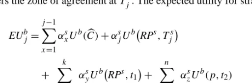
possible values for the seller’s deadline, it hasnstrategies to choose from. At timetduring negotiation, strategyS_jb is defined asIPb,RPs, T_js, Bfor all tT_js. At all later times, (i.e., betweenT_jsandT_ns) the strategy offers the price RPs. Thus the earliest time at which agreement can be reached using strategyS_jbisT_js and the latest time isT_ns. If the seller’s actual deadline is less thanT_js, thenS_jbresults in conflict. These strategies are depicted in Fig. 3(a). Out of these nstrategies, the one that gives the buyer the maximum expected utility(EUb_o)is its optimal strategy(S_ob). Agentb’s expected utility from strategyS_jb, is:

EUb_j=

j−1

x=1

α_xsUb(C) +α_jsUbRPs, T_js+

n

y=j+1

α_ysUbRPs, t (3)

whereT_jstT_ns.

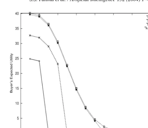
This is the general expression for the buyer’s EU from different strategies. Here, the value oft depends on the opponent’s strategy. In Section 3.5.2 we will explain how to obtain the value oft. For the present assume that this value is known to us. For this given value oft, the expected utility depends on the probability distribution (αs), the utility function (Ub), andj. For example, the EU for different values ofj between 1 and 15 is illustrated in Fig. 4. In this example,αs was defined as a Poisson distribution andδbwas 1.6 (a value greater than 1). As seen in the figure, EUb_j is maximum at j =7, indicating that the optimal time for entering the zone of agreement, denotedT_Js, isT₇s. The optimal strategy is thereforeS₇b. In this figure, the time points are at uniform discrete intervals. However, this is not necessary as long as the conditions for convergence of agents’ strategies (listed

Table 3

Optimal buyer strategies in different negotiation scenarios whenLsp contains a single element.T denotes the second time period, i.e., if negotiation begins at timet,T =t+1

Negotiation scenario Timetduring negotiation Optimal strategy

N1 tTJs IPb,RPs, TJs, B

t > T_Js RPs,RPs, Tns, L

N2 tTJs IPb,RPs, TJs, B

T_Js< tT_ks RPs,RPs, T_ks, L

t > T_ks RPs,RPb, Tb, B

N3 tTb IPb,RPb, Tb, B

N4 tT IPb,RPs, T , C

t > T RPs,RPs, Tns, L

N5 tT IPb,RPs, T , C

T < tT_ks RPs,RPs, T_ks, L

t > T_ks RPs,RPb, Tb, B

N6 tT IPb,RPb, T , C

t > T RPb,RPb, Tb, L

in Section 3.5.3) are satisfied. For a higher value ofδb, EUb_j is maximum at a higher value ofj. Lowering the value ofδb causes the peak of the curve to shift left. In other words

T_Js increases as δb increases and T_Js decreases asδb decreases. Forδb=1, EUb is at a maximum forj =1. This happens because the agent is indifferent to time. Higher values ofj result in some conflict situations and thus give a lower utility. But whenδb>1, the agent gains utility with time and the maximum utility is obtained forj >1.

The buyer’s optimal strategy for scenarioN1is listed in Table 3. LetSob(t)denote the price generated by the buyer’s optimal strategy at timet. The buyer’s action function for scenarioN1is defined as follows:

Abt, p_st_→b=

  

Quit ift > Tb_,

Accept ifp_st_→bSb

o(t), OfferS_ob(t)in the next time periodt otherwise.

In the definition of an agent’s action given in Section 3.1, the opponent’s offer is accepted if the utility from the opponent’s offer at timetis greater than or equal to the utility of the offer the agent is willing to generate at timet. But here, in order to decide when to accept the seller’s offer, the price offered by the seller at timet(p_st_→b) is compared with the price generated by the buyer’s optimal strategy (S_ob) at timet. This is because the seller’s actual deadline is not known to the buyer, andtcould be the seller’s deadline, in which case the seller quits and negotiation ends in a conflict if the buyer does not accept the offer at time

t. So even though the buyer’s utility increases with time, it has to accept the seller’s offer ifpt_s→bS_ob(t)and thereby avoid the chance of a conflict.

In scenario N2, the seller’s deadline can be either less than or greater thanTb. Since

than RPs. If an agreement is not reached by T_ks, it implies that the seller’s deadline is greater than Tb and to avoid conflict, the buyer needs to offer its reservation price RPb at Tb. Thus agentb should enter the zone of agreement at the latest possible time (to ensure that agreement is not reached earlier than that), remain at RPs untilT_ks and then offer/accept its own reservation price, RPb, atTb. The possible times for entering the zone of agreement areT₁s, . . . , T_ks. These strategies are depicted in Fig. 3(b), where strategyS_jb

enters the zone of agreement atT_js. The expected utility for strategyS_jbis:

EUb_j=

j−1

x=1

α_xsUb(C) +αs_jUbRPs, T_js

+ k

y=j+1

αs_yUbRPs, t1

+ n

z=k+1

αs_zUb(p, t2) (4)

where RPspRPbandT_jst1Tys andTjst2Tb.

As for scenarioN1, assume that the values ofp,t1, andt2, are known. In Section 3.5.2 we

will explain how to obtain these values. For the given values ofp,t1, andt2, the values

of EUb_j for different values ofj between 1 and 15 andδb_{=1.6 (whereα}s _{is a Poisson} distribution) are depicted in Fig. 5. As seen in the figure, the value ofj for which EUb_j is maximum depends on the value ofk. For higher values ofδb, we get the same pattern as in Fig. 5 but the peak of the curve shifts to the right. Lowering the value ofδbshifts the peak to the left. In other words, the optimal time (T_Js) for entering the zone of agreement increases asδb_{increases and decreases asδ}b_{decreases. Fig. 6 shows EU}b_forδb_{=1. As seen from} the figure, EUb is maximum at j =1. This happens because, for δb_{=1, the agent is}

Fig. 6. Buyer’s EU for different strategies in scenarioN2whenδb=1.

indifferent to time. Higher values of j result in some conflict situations and thus give a lower utility. But whenδb>1, the agent gains utility with time and the maximum utility is obtained forj >1. The buyer’s optimal strategy for scenarioN2is listed in Table 3. The

buyer’s action function for scenarioN2is the same as that for scenarioN1.

In scenarioN3, the buyer gains utility with time (i.e.,δb>1)andTb< T₁s. The buyer’s

optimal strategy here isS_ob= IPb,RPb, Tb, B. This strategy (shown in Fig. 3(c)) enters the zone of agreement at the latest possible time, which is close to the earlier deadlineTb, and thereby maximizes the time of agreement. It also optimizes the price of agreement by offering RPbonly atTb.

In the remaining three scenarios,N4toN6,δb<1 and the buyer loses utility with time.

In scenarioN4(shown in Fig. 3(d)), it is clear that the buyer can optimize both the price

and the time of agreement by offering RPs right from the beginning of negotiation, until

T_ns (see Table 3). Contrast this withS_obof scenarioN1, in which the zone of agreement is

entered atT_Js, whereas here it is entered at the beginning of negotiation using the Conceder function (sinceδb<1).

In scenario N5, the buyer’s optimal strategy is to offer RPs from the beginning of

negotiation until T_ks. If Ts T_ks, then negotiation ends at the latest byT_ks. Otherwise it continues beyond T_ks. The buyer then has to concede up to RPb in order to ensure agreement (see Fig. 3(e)). This strategy is listed in Table 3.

Finally, in scenario N6, the buyer’s optimal strategy is to offer RPb right from the

beginning of negotiation until Tb (see Fig. 3(f)). This is because when the buyer is in scenario N6, the possible scenarios for the opponent are N1, N2, N4 orN5. Since

buyer’s optimal strategies in all the six negotiation scenarios. The buyer’s action function in all the scenarios is the same as that for scenarioN1.

3.5.2. Optimal strategies for the buyer whenLs_pcontains more than one element

Optimal strategies for the buyer whenLs_p contains more than one element remain the same as those obtained in Section 3.5.1 in some, but not all, negotiation scenarios. Only those optimal strategies (listed in Table 3) that depend on the opponent’s reservation price change, while the others remain the same. More specifically, the optimal strategies in scenariosN3andN6remain the same, while those in scenariosN1,N2,N4, andN5change

whenLs_pcontains more than one element. We analyze each of these four scenarios below. The buyer’s action function,Ab, does not depend on the number of elements inLs_p and therefore remains the same as defined in Section 3.5.1 for all the scenarios.

As mentioned in Section 3.3, the information state of the buyer, Ib_{, hasn possible} values for the seller’s deadline andmpossible values for its reservation price. Also, recall that agentbbelieves thatβ_is is the probability that the opponent’s reservation price is RPs_i and thatα_js is the probability that the opponent’s deadline isT_js. The probability that the seller has the reservation price RPs_i and deadlineT_js is thus the product ofβ_is andα_js, and is denotedγ_i,js .

Consider scenarioN1first. The possible buyer strategies for this scenario are depicted in

Fig. 7. The number of possible strategies here ism×n. We useS_i,jb to denote the strategy that starts making offers at IPb, offers RPs_i atT_js using the Boulware function, and does not change the price thereafter. The strategy that yields the highest EU is the buyer’s optimal strategy. LetIandJ denote the values ofiandj that give agentbthe highest utility. Here we need to find these two values. Contrast this with the case whereLs_phad a single element which required finding only the optimal value ofj, i.e.,J.

The outcome of negotiation depends on both the buyer’s and the seller’s strategy. The buyer does not know the seller’s strategy, but it has two lotteries, Ls_p andLs_t, over the seller’s reservation price and deadline. So if the seller’s reservation price and deadline are

RP_isandT_js, then it plays strategyS_i,js that offers RPs_i atT_js. The probability with which the seller plays strategyS_i,js isγ_i,js . Thus although the buyer does not know the seller’s actual strategy, it knows that the seller can play m×n different strategies and the associated probabilities.

Consider the strategy S_m,nb . This strategy results in an agreement only if the seller’s actual reservation price is RPs_mand its deadline isT_ns. All the other values for the seller’s reservation price or deadline result in a conflict. Thus the EU from strategyS_m,nb is:

EUb_m,n=

m−1

x=1

n

y=1

γ_x,ys Ub(C) +

n−1

x=1

γ_m,xs Ub(C) +γ_m,ns UbRPs_m, T_ns. (5)

In general, strategyS_i,jb results in conflict if either the seller’s reservation price is higher than RPs_i, or its deadline is less thanT_js. The utility fromS_i,jb is therefore:

EUb_i,j=

i−1

c=1

n

d=1

γ_c,ds Ub(C) +

j−1

c=1

γ_i,cs Ub(C)

+γ_i,js UbRPs_i, T_js+

n

x=j+1

γ_i,xs UbRPs_i, t1

+ m

y=i+1 _j−1

z=1

γ_y,zs Ub(C) +γ_y,js Ubp1, Tjs

+ n

z=j+1

γ_y,zs Ub(p2, t2)

(6)

where RPs_yp1RPsi and RPsyp2RPsi andT_jst1TxsandT

s

j t2Tzs.

In the above expression, the values of p1 andp2depend on two factors: the opponent’s

strategy and the identity of the player that makes a move at the earlier deadline. The values oft1andt2depend only on the opponent’s strategy. Although the buyer does not know the

opponent’s actual strategy, it does know that the opponent will also behave strategically. This strategic behavior depends on the opponent’s scenario. Recall that when the buyer’s scenario isN1, the seller can be in any of the four scenarios:N2,N3,N5, orN6. We know

from Section 3.5.1 that in scenarioN6, an agent’s optimal strategy is to offer its reservation

price using the Conceder function. Thus if agentsis in scenarioN6, its optimal strategy is

to offer RPs using the Conceder function. In addition to the seller’s strategy, the values of

p1andp2also depend on who makes an offer at the earlier deadline. The player that makes

an offer at the earlier deadline could be the buyer or the seller, depending on who made the initial offer. Consider the case where it is the seller’s turn to make a move at the earlier deadline. The seller’s optimal strategy in scenarioN6is to offer RPs using the Conceder

function. As per the buyer’s action function, the buyer accepts the seller’s offer atT_js. We therefore getp1=p2=RPsy andt1=t2=T_js. On the other hand, if it is the buyer’s turn

accepts the buyer’s offer at timeT_js. This makesp1=p2=RPsi andt1=t2=Tjs. Using similar analysis, it can be seen that when agentsis in any of the remaining three scenarios (N2,N3, orN5), we getp1=p2=RPsy,t1=Txs, andt2=Tzsif the seller makes an offer at the earlier deadline; andp1=p2=RPs_i,t1=Txs, andt2=Tzs if the buyer makes an offer at the earlier deadline. The buyer knows who will make an offer at the earlier deadline, since the decision about which player will make the initial offer is made at the beginning of negotiation and thereafter players take turns alternately at each successive time period. Since the buyer does not know the seller’s scenario, we associate equal probabilities with each of the four possible seller’s scenarios,N1,N3,N5, andN6. Let eub1denote the value

of Eq. (6) when the seller’s scenario isN2,N3, orN5. Also, let eub₂denote the value of

Eq. (6) when the seller’s scenario isN6. The buyer’s EU therefore becomes:

EUb_i,j=3₄eu₁b+1₄eub₂. (7) The values ofiandj for which Eq. (7) is at a maximum are denotedI andJ. The buyer’s optimal strategy for scenarioN1, in terms ofI andJ, is listed in Table 4.

In scenarioN2, the buyer uses a strategySi,jb of the form depicted in Fig. 8. This strategy starts at IPb, offers RPs_i atT_js using the Boulware function, keeps the price constant at RPs_i untilT_ks, and thereafter uses the Boulware function again to offer RPbatTb. It is clear from Fig. 8 that ican vary between 1 andmandj can vary between 1 andk. Thus there are

m×kpossible strategies and the one that yields the maximum EU is the buyer’s optimal strategy. LetI andJdenote the values ofiandj respectively that give the highest utility. Here we need to find these two values. Contrast this with the case whereLs_phad a single element, which required finding onlyJ. The buyer’s EU from strategyS_i,jb is:

EUb_i,j=EUb₁+EUb₂+EUb₃. (8)

Table 4

Optimal buyer strategies in different scenarios whenLs_pcontains more than one element

Negotiation scenario Timetduring negotiation Optimal strategy

N1 tTJs IPb,RPsI, TJs, B

t > T_Js RPs_I,RPs_I, Tns, L

N2 tTJs IPb,RPsI, TJs, B

T_Js< tT_ks RPs_I,RPs_I, T_ks, L

t > T_ks RPs_I,RPb, Tb, B

N3 tTb IPb,RPb, Tb, B

N4 tT IPb,RPsI, T , C

t > T RPs_I,RPs_I, Tns, L

N5 tT IPb,RPsI, T , C

T < tT_ks RP_Is,RPs_I, T_ks, L t > T_ks RPs_I,RPb, Tb, B

N6 tT IPb,RPb, T , C

Fig. 8. The buyer’s strategyS_i,jb in scenarioN2whereLspcontains more than one element.

Here, the term EUb₁denotes agentb’s EU if the seller’s actual reservation price is higher than RPs_i, EUb₂denotes its EU if the seller’s actual reservation price is equal to RPs_i, and

EUb₃ denotes its EU if the seller’s actual reservation price is lower than RPs_i. We obtain each of these three terms below.

For EUb₁(i.e., for RPs >RPs_i), the seller’s deadline can be either less than or equal to

T_ks, or it can be greater than or equal toT_ks₊₁(see Fig. 8). IfTsT_ks, then negotiation ends in a conflict. EUb₁is therefore given by:

EUb₁=

i−1

x=1 _k

y=1

γ_x,ys Ub(C)+

n

y=k+1

γ_x,ys Ubp1, Tb

(9)

where(RPs_xp1RPb).

Note that the value of p1 depends on the opponent’s strategy and the identity of the

player that makes an offer at the earlier deadline. The four possible seller scenarios for the second term of Eq. (9) (i.e., Ts > Tb) are N1, N2, N4, or N5. For each of these

scenarios, the seller’s strategic behavior gives p1=RPb if the buyer makes a move at

the earlier deadline, andp1=RPbIif the seller makes a move at the earlier deadline. Note that in order to get these values for p1, the buyer and seller strategies need to converge

before the earlier deadline. The conditions for convergence of agents’ strategies are listed in Section 3.5.3. Also note that the value of RPb_I is present in the seller’s information state and is not known to the buyer. The buyer can therefore only takep1=RPbas the closest

approximation.

EUb₂=

j−1

x=1

γ_i,xs Ub(C) +γ_i,js UbRPs_i, T_js

+ k

x=j+1

γ_i,xs UbRPs_i, t1

+ n

x=k+1

γ_i,xs Ub(p2, t2) (10)

where(RPs_i p2RPb)and(Tjst1Txs)and(Tjst2Tb).

The possible scenarios for the seller for the third term of Eq. (10) areN2,N3,N5, orN6.

Considering the seller’s strategic behavior, we gett1=T_js if the seller’s scenario isN6and

t1=Txs otherwise. The possible scenarios for the seller, for the fourth term of Eq. (10), areN1,N2,N4, orN5. Considering the seller’s strategic behavior, we gett2=Tb for all

the four scenarios. The value ofp2depends on the player that makes a move at the earlier

deadline. If the buyer makes a move at the earlier deadline, we getp2=RPb. On the other

hand, if the seller makes a move at the earlier deadline we getp2=RPb_I. As forp1, since

the buyer does not know RPb_I, it can only takep2=RPbas the closest approximation for

all possible seller scenarios.

The last term, EUb₃(i.e., for the case RPs>RPs_i) is as follows:

EUb₃=

m

x=i+1 _j−1

y=1

γ_x,ys Ub(C) +γ_x,js Ubp3, Tjs

+ k

y=j+1

γ_x,ys Ub(p4, t3)+

n

y=k+1

γ_x,ys Ub(p5, t4)

(11)

where(RPs_xp3RPs_i)and(RPsxp4RPs_i)and

(RPs_xp5RPb)and(Tjst3Tys)and(Tjst4Tb).

The possible scenarios for the seller for the second and third terms of Eq. (11) areN2,N3,

N5, orN6, while for the fourth term they areN1,N2,N4, orN5. Considering the seller’s

strategic behavior we gett3=Tjs if the seller’s scenario isN6, andt3=Tys otherwise. For all the possible seller’s scenariost4=Tb. The values of p3, p4, and p5 depend on the

identity of the player that makes a move at the earlier deadline.p3=p4=RPsxif the seller makes a move at the earlier deadline, andp3=p4=RPs_i if the buyer makes a move at the

earlier deadline. Finally,p5=RPb_I if the seller makes a move at the earlier deadline and

p5=RPbif the buyer makes a move at the earlier deadline. Again, as forp1, the buyer can

only takep5=RPbas an approximation.

The buyer’s utility from strategyS_i,jb , is the sum of EUb₁, EUb₂, and EUb₃. Let eub₁denote the value of Eq. (8) if the seller’s scenario isN6, and eub₂denote its value otherwise. As

each of the four possible scenarios for the seller is equally probable, EUb_i,j becomes:

Fig. 9. The buyer’s strategy,Sb_i, whenLs_pcontains more than one element. (a) ScenarioN4. (b) ScenarioN5.

In the next scenario, i.e., N3, the buyer’s optimal strategy does not depend on the

opponent’s reservation price. Thus the buyer’s optimal strategy when Ls_p contains more than one element is the same as its optimal strategy whenLs_p contains a single element. This is also true for scenarioN6.

In negotiation scenario N4, the buyer’s optimal strategy is to offer the opponent’s

reservation price, RPs, immediately after negotiation starts and continue to offer the same price until negotiation ends. The possible strategies that the buyer can use whenLs_p has more than one element are of the formS_ib, where 1im. This is shown in Fig. 9(a). The buyer’s EU from strategyS_ibis:

EUb_i =

i−1

x=1

n

y=1

γ_x,ys Ub(C) +

n

x=1

γ_i,xs UbRPs_i, t1

+ m

x=i+1

n

y=1

γ_x,ys Ub(p1, t2) (13)

where RPs_xp1RPsi andT t1Txs andT t2Tys.

The values of t1 and t2 depend on the opponent’s scenario, while p1 depends on the

opponent’s scenario and the identity of the player that makes a move at T or the earlier deadline. If the opponent is in scenarioN6, then t1=t2=T . On the other hand, if the

seller’s scenario isN2,N3, orN5, thent1=Txsandt2=Tys. If the seller’s scenario isN6,

p1=RPsxif the seller makes a move at timeT andp1=RPs_i if the buyer makes a move

eub₂denote its value if the seller’s scenario isN2,N3, orN5. All the four possible seller’s

scenarios being equally probable, EUb_i becomes:

EUb_i =1₄eu₁b+3₄eub₂. (14) The buyer’s optimal strategy for scenarioN4is listed in Table 4.

Finally, in scenario N5 the buyer’s possible strategies are of the formSib shown in Fig. 9(b). The expected utility fromS_ibis:

EUb_i =

i−1

x=1 _k

y=1

γ_x,ys Ub(C)+

n

y=k+1

γ_x,ys Ubp1, Tb

+ k

x=1

γ_i,xs UbRPs_i, t1

+ n

x=k+1

γi,xUb(p2, t2)

+ m

x=i+1 _k

y=1

γ_x,ys Ub(p3, t3)+

n

y=k+1

γ_x,ys Ub(p4, t4)

(15)

where(T t1Txs)and(T t2Tb)and(T t3Tys) and(T t4Tb)and(RPsxp1RPb)and(RPsi p2RPb)

and(RPs_xp3RPsi)and(RPsip4RPb).

Using similar analysis, as for scenarioN2for the buyer, we get the following values. The

values of t1,t2,t3 andt4 depend on the seller’s scenario. We gett1=T if the seller’s

scenario is N6, andt1=Txs otherwise. We gett3=T if the seller’s scenario is N6, and

t3=Tys otherwise. Similarly, t2=t4=Tb for all possible seller scenarios. The values

ofp1,p2, andp4 depend on the identity of the player that makes a move at the earlier

deadline. The value of p3 depends on the identity of the player that makes a move at

T or the earlier deadline. We get p1=p2=p4=RPb if the buyer makes a move at

the earlier deadline, and p1=p2=p4=RPb_I if the seller makes a move at the earlier

deadline. Finally, p3=RPsx if the seller’s scenario isN6and the seller makes a move at

T . Butp3=RPs_i if the seller’s scenario isN6and the buyer makes a move atT . For the

remaining seller’s scenarios,p3=RPsx if the seller makes a move at the earlier deadline andp3=RPsi if the buyer makes a move at the earlier deadline. Since RPbIis not known to the buyer, it can only take RPbas the values ofp1,p2andp4. Let eub₁denote the value of

Eq. (15) if the seller’s scenario isN6, and eub₂denote its value otherwise. The expression

for EUb_i therefore becomes

EUb_i =1₄eu₁b+3₄eub₂. (16) The buyer’s optimal strategy for scenarioN5is listed in Table 4. Optimal strategies for the

3.5.3. Conditions for convergence of optimal strategies

It is clear from Section 3.5.2, that when both agents use their respective optimal strategies, the outcome of negotiation depends on RPs_I, T_Js, RPb_I, andT_Jb. For instance, consider the case where the buyer’s scenario isN1, andTJs has a value greater thanTs and

RPs_Ihas a value less than RPs. Here, the buyer starts at IPband uses the Boulware function to offer RPs_I at time T_Js. Agents quits at Ts and sinceTs < T_Js, negotiation ends in a conflict. Thus in scenarioN1, RPsI in the buyer’s optimal strategy should be greater than or equal to the seller’s actual reservation price (RPs) andT_Js should be less than or equal to the seller’s actual deadline (Ts) for the buyer and seller strategies to converge. Likewise, when the seller’s scenario isN1, RPbI in the seller’s optimal strategy should be less than or equal to the buyer’s actual reservation price andT_Jbin the seller’s optimal strategy should be less than or equal to the buyer’s actual deadline. The outcomes given in Table 6 will result only if the agents’ beliefs about each other satisfy the conditions for convergence of optimal strategies listed in Table 5. If these conditions are not satisfied, bargaining will end in a conflict. Furthermore, the more accurate agenta’s beliefs about agentaˆare, the closer

T_Jaand RPa_I are toTaand RParespectively.

The outcomes of negotiation, i.e., the price and time of agreement for all possible scenarios, when the conditions for convergence of optimal strategies are satisfied, are summarised in Table 6. For instance, consider row 1, where the buyer’s scenario is N1

and the seller’s scenario isN2. HereTs< Tbsince the buyer’s scenario isN1. The buyer’s

optimal strategy in scenario N1 is to offer a price lower than RPsm (whenever it is the buyer’s turn) at all timestless thanT_Js. At any timet greater than or equal toT_Js, the buyer accepts the seller’s offer if the seller offers a price lower than or equal to RPs_I; otherwise it offers RPs_I. Recall that in scenarioN2, the seller will always offer a price higher than RPs_I

beforeTsand offer RPs atTs. When the conditions for convergence of optimal strategies are satisfied, the possible values for the seller’s reservation price and deadline are shown in Fig. 10 as circles. One of the circles is the seller’s actual reservation price and deadline. Let

(RPs_c, T_ds)(shown as the shaded circle) be the seller’s actual reservation price and deadline. At timeT_ds it could be the buyer’s or the seller’s turn to make a move. Consider the case where it is the buyer’s turn atT_ds. As per its optimal strategy, the buyer offers RPs_I atT_ds

if the offer it receives in the previous time period is higher than IPb. In scenarioN2, the

price that the seller offers in the previous time period lies in the range [RPb₁,RPb_m], i.e.,

Table 5

Conditions for convergence of optimal strategies

Negotiation scenario Condition for convergence

Buyer’s strategy Seller’s strategy

N1 RPsIRPsandTJsTs RPbIRPbandTJbTb

N2 RPsIRPsandTJsTs RPbIRPbandTJbTb

N3 None None

N4 RPsIRPs RPbIRPb

N5 RPsIRPs RPbIRPb