PP 2014 16: Measuring Diversity of Preferences in a Group

Measuring Diversity of Preferences in a Group

Vahid Hashemi

and

Ulle Endriss

Abstract. We introduce a general framework for measuring the degree of diversity in the preferences held by the members of a group. We formalise and investigate three specific approaches within that framework: diversity as the range of distinct views held, diver-sity as aggregate distance between individual views, and diverdiver-sity as distance of the group’s views to a single compromise view. While similarly attractive from an intuitive point of view, the three ap-proaches display significant differences when analysed using both the axiomatic method and empirical studies.

1

INTRODUCTION

Preferences are ubiquitous in AI [5, 12]. Examples for application domains include recommender systems, planning, and configuration. Of particular interest is the case of preference handling in multiagent systems, where several agents each have their own individual prefer-ences and we need to take decisions that are appropriate in view of such a profile of preferences. The normative, mathematical, and algo-rithmic aspects of this problem are studied in the field of (computa-tional) social choice [3]. In social choice, preferences are taken to be linear orders over a finite set of alternatives. As is well known, many of the most interesting phenomena in social choice are in fact rare events. For example, while the notoriousCondorcet Paradox man-ifests itself in around 25% of all theoretically possible preference profiles for 5 alternatives and a large number of voters, empirical studies suggest that it plays hardly any role in real-world elections of the same size [11, 17]. Another example is the fact that many of the computational hardness results for the strategic manipulation prob-lem in voting rely on a very narrow basis of worst-case scenarios, while the vast majority of problem instances are in fact easy [18].

This divergence can be explained by the fact that the prefer-ence profiles we encounter in practice exhibit a certain amount of structure. The classical approach to modelling such structure are domain restrictions, the best known example of which is single-peakedness[9]. Yet, while an unconstrained model of social choice arguably is too broad, domain restrictions are often too narrow to accurately describe preference profiles that occur in practice. In this paper, we propose the exploration of a middle way. Our starting point is the basic idea that the lessdiversethe preferences in a profile are, the easier it should be to come to a mutually acceptable decision. For example, in the most extreme case where all agents share the exact same preference order, it will be trivial to make collective decisions.

Vice versa, the more diversity we find in a profile, the more we should expect to encounter paradoxes, i.e., situations in which different so-cial choice-theoretic principles would lead to opposing conclusions.

Our first contribution is to propose a formal model of preference diversity. At the centre of this model is the notion of preference

1_{Institute for Logic, Language and Computation, University of Amsterdam,} email: [email protected], [email protected]

diversity index(PDI): a function mapping profiles to nonnegative numbers, with 0 denoting perfect agreement amongst all agents. The model does not commit to one specific interpretation of the term di-versity. Rather, we use it to formalise three concrete interpretations: diversity as the range of distinct views held (support-based PDI), diversity as aggregate distance between individual views ( distance-basedPDI), and diversity as distance of the group’s views to a single compromise view (compromise-basedPDI).

We formulate several intuitively appealing properties of PDI’s as

axiomsand classify our concrete indices in terms of which of these axioms they satisfy. We also provide an example for animpossibility result, showing that certain axioms are mutually incompatible, and a

characterisation result, showing how one concrete PDI is fully de-termined by a certain combination of axioms. On the practical side, we have conducted a range ofexperimentsthat shed additional light on our PDI’s. In particular, we explore how the differences between synthetically generated preference data and data sampled from a real election profile manifest themselves in terms of the distribution of diversity over profiles. We also confirm that the likelihood for unde-sirable social choice-theoretic effects increases with diversity.

In Section 2 we introduce our model of preference diversity and define several specific PDI’s. Section 3 is devoted to the axiomatic analysis of diversity and Section 4 presents our experimental results. We conclude with a discussion of related work in Section 5 and a brief outlook on other approaches to defining PDI’s in Section 6.

2

MEASURING PREFERENCE DIVERSITY

In this section we introduce the concept ofpreference diversity index

(PDI) and then define several concrete such indices.

2.1

Basic terminology and notation

LetX be a finite set ofm alternatives. We modelpreferencesas (strict)linear ordersover the set of alternatives (recall that a linear or-derRis a binary relation that is irreflexive, transitive, and complete). We writeL(X)for the set of all preference/linear orders overX. The

positionofx∈ XinR∈ L(X)is pos_R(x) =|{y∈ X |yRx}|. LetN ={1, . . . , n}be a finite set ofvoters(oragents). Aprofile

R= (R1, . . . , Rn)∈ L(X)nis a vector of preference orders, one for each voter. We writeNR

xy = {i ∈ N | xRy}for the set of voters who in profileRsay that they preferxovery. Thesupportof a profileR= (R1, . . . , Rn)is the set of preference orders occurring in it: SUPP(R) ={R1}∪· · ·∪{Rn}. We call a profileRunanimous if|SUPP(R)|= 1, i.e., if it is of the form(R, . . . , R).

2.2

Preference diversity orderings and indices

about which of them we consider more diverse. Recall that aweak orderis a binary relation that is reflexive, transitive, and complete.

Definition 1. Apreference diversity order(PDO) is a weak order<

declared on the space of preference profiles L(X)n that respects

R<(R, . . . , R)for allR∈ L(X)n

and allR∈ L(X).

That is, any PDO is required to classify unanimous profiles as being minimally diverse (and any two such profiles are equally diverse). We writefor the strict part of<, and∼for its indifference part.

Definition 2. Apreference diversity index(PDI) is a function∆ :

L(X)n_→

R+∪ {0}, mapping profiles to the nonnegative reals, that respects∆(R, . . . , R) = 0for anyR∈ L(X).

Letmax(∆) = max{∆(R)|R∈ L(X)n}. We say that a PDI∆is

normalisedif it maps any given profile to the interval[0,1], and the maximum of 1 is reached for at least one profile, i.e.,max(∆) = 1. Every given PDI∆gives rise to a normalised PDI∆0by stipulating

∆0(R) = ∆(R)/max(∆)for every profileR∈ L(X)n. A PDI∆induces a PDO<∆

, by stipulatingR<∆_R0

if and only if∆(R) >∆(R0)for any two profilesR,R0 ∈ L(X)n. Observe that, as∆is required to map any unanimous profile to 0, any such profile will be correctly placed at the bottom of the corresponding PDO<∆(i.e., the two definitions match). Every PDO<(and thus every PDI) defines a partitioning ofL(X)n

into equivalence classes w.r.t.∼. We can think of these equivalence classes as the possible

levelsof diversity. Let thedimensionof a PDI/PDO be the number of equivalence classes it defines (for fixednandm).

2.3

Specific preference diversity indices

We now introduce three specific approaches to defining PDI’s. The first approach is based on the idea that diversity may be measured in terms of thenumber of distinct viewsrepresented within a group. In its simplest form, this means that we count the number of distinct preference orders in a profile. This leads to thesimple support-based PDI∆suppwith∆supp(R) =|SUPP(R)| −1(we subtract 1 to ensure ∆supp(R, . . . , R) = 0). We can generalise this idea and count the

number of distinct ordered k-tuples of alternatives appearing in a profile. The number of such tuples inonepreference order is m_k. LetLk(X)denote the set of orderedk-tuples of alternatives.

Definition 3. For a givenk6m, thesupport-based PDI∆`=ksuppmaps

any given profileR∈ L(X)nto the following value:

∆`=ksupp(R) = |{T∈ Lk(X)|T ⊆Rifor somei∈ N }| − m_k

For example,∆`=2suppcounts the number of ordered pairs at least one

agent accepts (above and beyond m_k

). Note that∆supp≡∆`=msupp.

Our second approach is based on the idea that diversity is related to thedistances between the individual viewsheld by the members of a group. We first require a notion of distance between two single preference ordersRandR0, i.e., a functionδ:L(X)× L(X)→R

meeting the familiar axioms for distances (nonnegativity, identity of indiscernibles, symmetry, and the triangle inequality). The following are all standard definitions that are widely used in the literature [6, 8]:

• Kendall’s tau:K(R, R0) =1₂·(|R\R0|+|R0\R|)

• Spearman’s footrule:S(R, R0) =P

x∈X|posR(x)−posR0(x)| • Discrete distance:D(R, R0) = 0ifR=R0, and= 1otherwise

WhenRandR0are linear orders, our definition forKis equivalent to the more commonK(R, R0) =1

2· |{(x, y)|xRyandyR

0

x}|. Note

that we divide by 2 to ensure we count ordered pairs, not merely pairs of alternatives. To lift distances between pairs of voters to distances between the members of a group, we can use any aggregation opera-torΦ :Rn×n→R(that is nondecreasing, associative, commutative,

and has identity element 0), such asmaxorΣ(sum).

Definition 4. For a given distanceδ : L(X)× L(X) → Rand

aggregation operatorΦ :Rn×n→R, thedistance-based PDI∆Φ,δ_dist

maps any given profileR∈ L(X)nto the following value:

∆Φ,δ_dist(R) = Φ(δ(Ri, Ri0)|i, i0∈ N withi < i0)

That is, we first compute then(n−1)/2-vector of pairwise distances

δ(Ri, Ri0)and then applyΦto that vector. The PDI∆Σ,K

dist, for

in-stance, measures diversity as the sum of the Kendall tau distances between all pairs of preferences in a profile. In this paper, we will largely focus onΦ = Σand the effect of varyingδ.

The idea underlying our third approach is to measure diversity as a group’s accumulateddistance to a compromise view. For in-stance, for a given profileR, we may compute itsmajority graph

MG(R) ={(x, y) | |NxRy|> n₂}and then measure the distance

of the individual preferences to the compromise view represented by MG(R). To measure the distance between a preference order and a compromise view, we will use the Kendall tau distance, although in principle also other distances could be used. Observe thatK, as defined above, is a meaningful notion of distance between any two binary relations onX, not just linear orders. We refer to functions mapping profiles to binary orders (representing compromise views) associal welfare functions(SWF), which is a slight generalisation of the common use of the term in social choice theory [10].

Definition 5. For a given SWFF :L(X)n _{→ 2}X ×X

and aggre-gation operatorΦ :Rn×n→R, thecompromise-based PDI∆Φ,Fcom

maps any given profileR∈ L(X)n

to the following value:

∆Φ,Fcom(R) = Φ(K(Ri, F(R))|i∈ N)

Thus,∆Σ,MGcom , for instance, computes the sum of the distances of the

individual preferences to the majority graph. BesidesF=MG, we can use voting rules, e.g., theBorda rule[10], to define a compro-mise. Under Borda, each voterigives as many points toxas there are other alternatives belowxini’ranking; the Borda score ofxis the sum of those points. This induces a SWF that for any given pro-fileRreturns the weak orderBor(R) ={(x, y)|BordaScore(x)>

BordaScore(y)}. Thus, the PDI∆max,Bor

com computes the maximal

dis-tance of any individual preference order to the ranking we obtain when we order alternatives in terms of their Borda score.2

3

AXIOMATIC ANALYSIS

In this section we motivate and formalise desirable properties that a specific manner of measuring preference diversity may or may not satisfy. That is, in the parlance of social choice theory [10], we in-troduce a number ofaxiomsfor preference diversity. We formulate these axioms in terms of PDO’s rather than PDI’s, i.e., we axioma-tise the ordinal notion of “being more diverse than”, rather than the cardinal notion of having a particular degree of diversity. The reason for this choice is that, while some details of the numerical representa-tion of degrees of diversity is bound to be arbitrary, relative diversity

2_{Beware that this approach does not result in a well-defined PDI for every} possible voting rule: e.g., if we rank alternatives in terms of theirplurality

judgments should not and need not be. Our axioms will nevertheless apply to PDI’s indirectly, given that every PDI induces a PDO.

We then use our axioms to organise the space of concrete ways of measuring preference diversity introduced earlier. We will also see that not all combinations of axioms can be satisfied together.

3.1

Axioms

Our first axiom is a basic symmetry requirement w.r.t. voters.

Axiom 1. A PDO< isanonymousif, for every permutationσ :

N → N, we have(R1, . . . , Rn)∼(Rσ(1), . . . , Rσ(n)).

The statement above is understood to apply toall preference pro-files(R1, . . . , Rn). For the sake of readability, we shall keep such universal quantification over profiles implicit also in later axioms. Our next axiom, neutrality, postulates symmetry w.r.t. alternatives. For any permutationτ :X → Xon alternatives and any preference orderR∈ L(X), defineτ(R) ={(x, y)|τ(x)Rτ(y)}.

Axiom 2. A PDO<isneutralif, for every permutationτ :X → X, we have(R1, . . . , Rn)∼(τ(R1), . . . , τ(Rn)).

Our next axiom says that no two profiles should be judged as being of equal diversity, unless anonymity and neutrality force us to do so.

Axiom 3. A PDO<isstrongly discernibleifR∼R0impliesR= (τ(R0σ(1)), . . . , τ(R

0

σ(n)))for someσ:N → N andτ :X → X.

Strong discernability is a demanding requirement. Intuitively speak-ing, it excludes PDO’s with a low dimension. The next axiom is much weaker (and implied by strong discernability). It only requires the bottom level to be distinct from the others.

Axiom 4. A PDO<isweakly discernibleifRbeing unanimous and

R0not being unanimous together implyR0R.

One possible position to take would be to say that diversity should be a function of the variety of views taken by members of a society, but that it should not depend on the frequency with which any particular such view is taken. That is, one might argue, the level of diversity of a profile should only depend on its support.

Axiom 5. A PDO<issupport-invariantifSUPP(R) =SUPP(R0)

impliesR∼R0.

Observe that support-invariance implies anonymity. A different po-sition to take would be to say that every single preference order mat-ters. That is, it should not be possible to determine the level of diver-sity of a profile by only inspecting a proper subset of its elements.

Axiom 6. A PDO < is nonlocal if for every profile R = (R1, . . . , Rn)∈ L(X)nand every voteri∈ Nthere exists an order

R0∈ L(X)such thatR6∼(R1, . . . , Ri−1, R0, Ri+1, . . . , Rn).

Our next axiom is adopted from the literature on ranking opportunity sets for measuring freedom of choice [16]. For any profileRforn

voters and individual preferenceR, letR⊕R= (R1, . . . , Rn, R)be the profile forn+1voters we obtain by addingRto the first profile.3

Axiom 7. A PDO<isindependentif it is the case thatR<R0if and only ifR⊕R<R0⊕Rfor every two profilesR,R0∈ L(X)n

and every preferenceR6∈SUPP(R)∪SUPP(R0).

3_{Note that, strictly speaking, Axiom 7 speaks about afamilyof PDO’s (one} for eachn), even if it does not directly compare profiles of different size.

Finally, we consider two possible definitions ofmonotonicity. What they have in common is that they identify situations in which one or more voters change their preferences by moving closer to the views of the rest of the group, which intuitively should reduce diversity. First, suppose a single voter abandons her own preference order and instead adopts the preferences of one of the other voters.

Axiom 8. A PDO<ismonotonicifR<R0whenever there exist

j, k∈ N such thatR0j=RkandR0i=Rifor alli6=j.

Observe that our monotonicity axiom implies support-invariance: if SUPP(R) =SUPP(R0), then we can move fromRtoR0(andvice versa) via a sequence of monotonicity-moves.

Now suppose one or several voters each swap two adjacent alter-nativesxandyin their preference orders. Under what circumstances should we consider such a move as having reduced diversity?

Axiom 9. A PDI<isswap-monotonic ifR < R0 holds when-ever there exist alternativesx, y ∈ X such that|NxRy|> |NyRx|, NxR0y=N, andNwRz =NR

0

wzfor all{w, z} 6={x, y}.

That is, (a) before the move fromRtoR0there is a (possibly weak) majority forx y, (b) after the moveallvoters agree onx y, and (c) no other relative rankings change in the process. The axiom says that such a move decreases (or at most maintains) diversity. This axiom is relatively weak: it only applies if every voter either already ranksxabovey, or if she ranksydirectlyabovexand thus has the opportunity to swap them without affecting other rankings.

3.2

Results

Which PDO’s satisfy which axioms? First, there is a group of three very weak axioms that will be satisfied by any reasonable PDO. In particular, as is easy to check, they are satisfied by the three specific families of PDO’s defined in Section 2.3.

Fact 1. Every PDO induced by a PDI of the form∆`=k

supp,∆

Φ,δ

dist, or ∆Φ,Fcom withk ∈ {1, . . . , m},Φ∈ {Σ,max},δ ∈ {K, S, D}, and Fbeing an anonymous and neutral SWF is anonymous, neutral, and weakly discernible.

At the other extreme, the axiom of strong discernability is not satis-fied by any of our specific PDO’s. The following impossibility result illustrates the overly demanding character of this axiom.

Proposition 2. Form > 2 andn > m!, no PDO can be both support-invariant and strongly discernable.

Proof. We first derive anupper boundon the dimension of any PDO that is support-invariant. The number of possible preference orders ism!. A support-invariant PDO has to determine the level of a given profileRbased on SUPP(R) alone. There are2m!_−1nonempty subsets of the set of all possible preferences, i.e., there are at most

2m!_{−1possible sets of support. Hence, the maximal dimension of} any support-invariant PDO is2m!−1.

Next, we derive alower boundon the dimension of any PDO that is strongly discernable. There are(m!)n

distinct profiles. Let us first partition this space into clusters of profiles such that any two profiles that are reachable from one another via a permutation on agents are placed into the same cluster. There are m!_n

= m!+n_n−1 such clusters:4for each of them!possible preferences we have to decide

4_{Recall from basic combinatorics that} n k

= n+k_k−1

how many agents should hold that preference, with the total num-ber of agents adding up ton. Let us now again partition this space of clusters into larger clusters, such that any two profiles reachable from each other via a permutation of alternatives are also in the same clus-ter. The number of these clusters is the lowest possible dimension of any PDO that is strongly discernible. Computing this number is a demanding combinatorial problem that has been studied, amongst others, by E˘gecio˘glu [7]. Closed formulas are known only for certain special cases. However, for our purposes a lower bound is sufficient. There arem!possible permutations of the alternatives. Hence, each of the large clusters can contain at mostm!of the small clusters. Thus, m!_n/m!is a lower bound on the number of clusters.

m! n

m! =

m! +n−1

n ×

m! +n−2 n−1 × · · · ×

m! + 1 2

> m! +m!

m! + 1 ×

m! +m!−1 m! × · · · ×

m! + 1 2

The denominator of the leftmost factor is equal to the numerator of the rightmost one. So we can rewrite asQm!

i=2 m!+i

i . Now, all of the

m!−1factors of this product are at least equal to 2. The first one (withi= 2) furthermore is at least equal to 4 (form >2). Hence,

m! n

/m! > 2m!. This concludes the proof, as it shows that the upper bound is strictly smaller than the lower bound derived.

Our next result is a characterisation of the simple support-based

PDO, i.e., the PDO induced by∆`=m

supp. That is, this is the PDO<

defined asR < R0if and only if|SUPP(R)| > |SUPP(R0)|. As we shall see in Section 5, this result is closely related to a classical theorem on ranking opportunity sets due to Pattanaik and Xu [16].

Proposition 3. A PDO is support-invariant, independent, and weakly discernible if and only if it is the simple support-based PDO.

Proof (sketch). First, observe that the simple support-based PDO clearly satisfies all three axioms. For the other direction, let<be any PDI that is support-invariant, independent, and weakly discernible. We need to show that R < R0 if and only if |SUPP(R)| > |SUPP(R0)|. This is equivalent to proving the following two claims:

(1) |SUPP(R)|=|SUPP(R0)|impliesR∼R0. (2) |SUPP(R)|=|SUPP(R0)|+ 1impliesRR0.

We shall make repeated use of the following fact: By support invari-ance, for every profileRand every preferenceR∈SUPP(R), there exists a profileR0of the same size that has the same support and in whichRoccurs exactly once.

We first prove claim (1) by induction onk=|SUPP(R)|. Ifk= 1, then both profiles are unanimous and we are done. Now assume the claim holds forkand consider two profilesRandR0with support of sizek+1. First, supposeRandR0share at least one preference

R. W.l.o.g., assumeRoccurs exactly once in each of them. LetRˆ be the rest ofRand letRˆ0be the rest ofR0, i.e.,R = Rˆ⊕R, R0=Rˆ0⊕R, andR6∈SUPP(Rˆ)∪SUPP(Rˆ0). AsRˆ∼_Rˆ0

by the induction hypothesis, we thus obtainR∼R0from the left-to-right direction of the independence axiom. In caseRandR0do not share any single preferenceR, this construction is not applicable. In this case, letRbe a preference with single occurrence inRand letRˆ be such thatR=Rˆ⊕R. Now considerR0andRˆ⊕R0for some

R0 ∈ SUPP(R0). These two profiles do share a preference, so we haveR0 ∼_Rˆ_⊕R0

. We can then repeat the same argument forR andR⊕ˆ R0, which also share a preference, and obtainR∼R⊕ˆ R0. Thus,R∼R0follows in all cases.

For claim (2), we can use the same technique. For the base case of the induction we now use weak discernability to show thatR R0when|SUPP(R)|= 2and |SUPP(R0)|= 1. For the induction step we now use the right-to-left direction of independence (which is equivalent to the left-to-right direction forrather than<).

We stress that the crucial axiom in this last result is independence. In particular, support-invariance only says that a profile’s diversity must be computable from its support, but it does not say that the support’s cardinality needs to play any role in this process.

So far we have discussed our weakest and our most restrictive ax-ioms. The remaining axioms tend to be satisfied by some reasonable PDO’s and not by others, which means that they are helpful in struc-turing the space of all reasonable PDO’s. For the main specific PDI’s considered in this paper (and, more precisely, for the PDO’s they in-duce), Table 1 summarises which of them satisfy which axioms. In the interest of space, we do not include proofs for the claims made in the table, but in most cases these claims are relatively easy to verify. Note that in some cases we state a sufficient (not always necessary) condition for a particular PDI to satisfy a particular axiom. For ex-ample, swap-monotonicity is satisfied by a compromise-based PDI if the SWF it is based on satisfies thePareto principleand Arrow’s

independence of irrelevant alternatives[10]. Strong discernability is omitted from the table, as it is not satisfied by any of our PDI’s.

∆`=k

supp ∆

Σ,δ

dist ∆

max,δ

dist ∆

Σ,F

com ∆

max,F

com

Support-invar. X × X × ×

Nonlocality n6k! X × X ×

Independence k=m × × × ×

Monotonicity X × X × ×

Swap-monoton. X δ=K δ=K Fis Arrovian

Table 1. Classification of PDI’s in terms of axioms.

4

EXPERIMENTAL ANALYSIS

In this section, we report on an experimental analysis of our PDI’s. The experiments conducted fall into two classes. In the first kind of experiment we draw profiles from a given distribution and plot di-versity values against the frequency of drawing profiles with these values. In the second kind, we investigate to what extent increas-ing diversity correlates with an increase of unwanted social choice-theoretic effects, such as the existence of Condorcet cycles.

Our findings are relative to the distribution over preference pro-files from which we sample. We use two distributions. The first is the synthetic distribution generated by theimpartial culture assump-tion(IC). This is the assumption that every possible profile is equally likely to occur. Despite its well-known limitations [17], this is the most widely used assumption in experimental work on social choice theory and serves as a useful base line. To generate the second dis-tribution we have sampled from the (second)AGH Course Selection

dataset available from PREFLIB, an online library of datasets con-cerning preferences [13]. This is a dataset with the complete prefer-ences of 153 students regarding 7 course modules, collected at AGH University of Science and Technology, Krak´ow, in 2004. We have generated profiles by choosing, uniformly at random, 50 individual preferences regarding the first 5 courses.

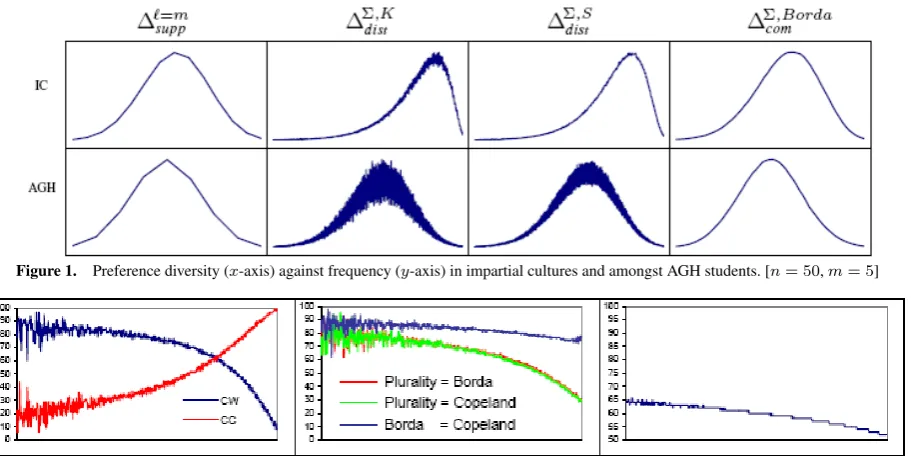
Figure 1. Preference diversity (x-axis) against frequency (y-axis) in impartial cultures and amongst AGH students. [n= 50,m= 5]

Figure 2. Diversity for∆Σ,K_dist / IC data (x-axis). Condorcet winners/cycles; agreement between voting rules; voter satisfaction (y-axis). [n= 50,m= 5]

profiles from the relevant distribution. However, for most PDI’s, pro-files with very low or very high diversity have extremely low proba-bility of occurring. For example, onlym!in(m!)n

profiles are unani-mous and thus have diversity 0 under every PDI. To be able to present our data in an illustrative manner, we therefore apply the following

pseudo-normalisation. For a given PDI∆and a given sample of pro-files, letαminbe the largest real number such that at most1hof the profiles have a diversity value belowαmin. Analogously, letαmaxbe the smallest real number such that at most1hof the profiles have a diversity value aboveαmax. We then plot the pseudo-normalised PDI∆0with∆0(R) = ∆(R)−αmin

αmax−αmin. Note that, strictly speaking,∆

0

is not a PDI itself, as it can return values below 0. Also, as we plot diversity values from 0 to 1 only, up to2hof the data may not be shown. What we gain in return is that we do not need to plot very long tails that only represent insignificantly small amounts of data. For all our plots, thex-axis ranges from 0 to 1.

4.1

Diversity distribution across cultures

Figure 1 shows, for both the IC and the AGH data, the relative frequency of each diversity value for four of our PDI’s. Recall that each plot is showing around 99.8% of the data, after pseudo-normalisation. We can make two observations. First, all four PDI’s result in what we judge to be reasonable frequency distributions, for both IC and AGH: very high and very low diversity are very rare, and there is a clear peak. Second, the AGH data results in a distribution where the peak is further to the left than for the IC data. This is what we would expect, and what we would want a good PDI to show: real preference profiles have more internal structure than purely random data, so we would expect to see less diversity. The simple support-based PDI is least able to show this difference.

A feature of the data that, due to our pseudo-normalisation, is not shown in Figure 1 is the number of distinct levels that the 1 million profiles we sampled ended up in. This data is shown, for the four PDI’s of Figure 1 and five additional ones, in Table 2. We can make two observations. First, the support-based PDI’s and the distance-based PDI using themax-operator make use of very few levels. This arguably makes them less attractive than the other PDI’s. Second, the range of levels used is generally (much) larger for the AGH data than

for the IC data (which explains the increased levels of noise for the AGH data in Figure 1). In particular, an IC profile is very unlikely to have very low diversity. Thus, the range of levels observed is another criterion we can use to tell apart synthetic data and data based on real preferences. Overall, the distance-based PDI’s using theΣ-operator for aggregation emerge as the most useful PDI’s.

PDI IC AGH PDI IC AGH PDI IC AGH

∆`=m

supp 22 13 ∆

Σ,D

dist 34 244 ∆

Σ,Bor

com 84 85

∆`=2

supp 1 2 ∆

Σ,S

dist 462 1170 ∆

Σ,MG

com 94 88

∆`=3

supp 4 12 ∆

Σ,K

dist 660 1561 ∆

max,K

dist 2 3

Table 2. Observed number of levels (n= 50,m= 5).

4.2

Impact on social choice-theoretic effects

Intuitively speaking, the less diverse a profile, the better behaved it should be from the perspective of social choice theory. Next, we re-port on three experiments where we put this intuition to the test for the PDI∆Σ,K_dist and data generated using the IC assumption. The re-sults are shown in Figure 2 (diversity values against percentages).

In the first experiment we have measured the frequency of observ-ing anCondorcet cycle(a cycle in the majority graph) in a profile and the frequency of a profile having aCondorcet winner(an alternative that wins against any other alternative in a pairwise majority con-test).5Figure 2 shows that, as diversity increases, so does the prob-ability of encountering a Condorcet cycle, while the probprob-ability of finding a Condorcet winner decreases. This is exactly the behaviour we would like a good PDI to display, as it helps us predict good and bad social choice-theoretic phenomena.

The second experiment concerns the extent to which different vot-ing rules agree on the winner for a given profile. For twoirresolute

voting rules, which may sometimes return a set of tied winners, we require a suitable definition for their degree of agreement under a given profile. For voting rulesF1 andF2, letW1 andW2 be the sets of winners we obtain. We define theirdegree of agreementas

|W1∩W2|

|W1|×|W2|. This is the probability of picking the same unique

win-ner if each voting rule were to be paired with a uniformly random tie-breaking rule. Figure 2 shows the average degree of agreement for profiles with a given PDI-value for three pairs of well-known vot-ing rules [10]: Plurality/Borda, Plurality/Copeland, Borda/Copeland. The plurality rule is widely regarded as a low-quality rule and this shows also here, as it disagrees considerably with the other two rules. This effect increases drastically as diversity increases.

Finally, we have computed the averagevoter satisfactionunder the Borda rule. To this end, we define the satisfaction of a voter as the number of alternatives she ranks below the Borda winner. When normalised to percent, a unanimous profile would result in a satisfac-tion of 100%, while a satisfacsatisfac-tion below 50% is not possible for the Borda rule. Figure 2 again clearly shows how voter satisfaction de-creases with increased diversity and how it gets close to the absolute minimum of 50% for very high (and rare) values of diversity.

5

RELATED WORK

Our model is related to the literature onfreedom of choiceconcerned with the ranking of alternative opportunity sets [15, 16], dealing with questions such as whether a choice between a bike and a car pro-vides more freedom than the choice between a red car and a blue car. Conceptual differences aside, an important mathematical difference between ranking opportunity sets and ranking preference profiles in terms of diversity is that we only compare profilesof the same size, while two opportunity sets to be compared may have different car-dinalities. This means that no direct transfer of results is possible. Still, a seminal result in this field, due to Pattanaik and Xu [16], has inspired our Proposition 3. They show that the only method of rank-ing opportunity sets satisfyrank-ing three basic axioms they propose is the method of simply counting the number of options in each set. Their axioms areindependence(of which ours is a direct translation), indif-ference between no-choice situationsrequiring any two singletons to be ranked at the same level (this requirement is part of our definition of a PDI), and astrict monotonicityaxiom comparing sets of cardi-nality 1 and 2. The latter is not meaningful, or even expressible, in our framework. However, our weak discernability axiom has similar consequences. Pattanaik and Xu interpret their result as an impos-sibility result, given that simply counting opportunities is an overly simplistic way of measuring freedom of choice. As our empirical re-sults suggest that the simple support-based PDI is not very attractive, Proposition 3 may be also be considered an impossibility result.

More expressive models of diversity, such as the multi-attribute approach of Nehring and Puppe [15] with its applications to the study of biodiversity, are not directly comparable to our setting.

Most closely related to our model is recent work on the cohesive-ness(or the degree of consensus) of a profile [1, 2], which is the opposite of our notion of diversity. These studies focus on a gen-eralisation of the Kendall tau distance, i.e., on measures based on averaging over pairwise distances between preferences (which can be seen as a special case of our distance-based measures) or the dual of this definition (averaging over the differences in the support of all possible pairs of alternatives). They also define several axioms (sim-ilar to some of ours) that characterise this class of measures. They do not, however, study the relationship between cohesiveness and social choice-theoretic phenomena.

Our compromise-based PDI’s are related todistance-based ratio-nalisationsof voting rules [8, 14]. Such a rationalisation consists of a distance measure and a notion of consensus profile (e.g., a unanimous profile or one with a Condorcet winner): the winners are the

alterna-tives that win in the consensus profile that is closest (in terms of the distance measure) to the actual profile. What our compromise-based PDI’s measure is precisely such a distance to a unanimous profile.

6

CONCLUSION

We have introduced the concept ofpreference diversity, together with a formal model facilitating the analysis of this concept. Besides being of interest in its own right, we also hope that PDI’s may serve as a useful tool for parameterising data in research on preference handling and social choice, including applications in AI.

In the interest of space, we have focussed on three families of spe-cific PDI’s, but there is in fact a rich landscape of additional options that should be investigated in depth. For instance, we may count the maximal number preferences sharing a common subpreferences of a given length`; we may measure the maximal distance between all preferences in a given profile and all preferences not in the profile (to see how close a profile is to covering the full space of possibilities); or we may measure the distance to a single-peaked profile. In fact, the latter is a problem that already has received some attention in the lit-erature [4]. Finally, we may use other distances and other aggregation operators (e.g., max-of-min) than those mentioned in Section 2.3.

REFERENCES

[1] J. Alcalde-Unzu and M. Vorsatz, ‘Measuring the cohesiveness of prefer-ences: An axiomatic analysis’,Social Choice and Welfare,41(4), 965– 988, (2013).

[2] R. Bosch,Characterizations of Voting Rules and Consensus Measures, Ph.D. dissertation, University of Tilburg, 2006.

[3] F. Brandt, V. Conitzer, and U. Endriss, ‘Computational social choice’, inMultiagent Systems, ed., G. Weiss, 213–283, MIT Press, (2013). [4] R. Bredereck, J. Chen, and G. J. Woeginger, ‘Are there any nicely

struc-tured preference profiles nearby?’, inProc. 23rd International Joint Conference on Artificial Intelligence (IJCAI), (2013).

[5] C. Domshlak, E. H¨ullermeier, S. Kaci, and H. Prade, ‘Preferences in AI: An overview’,Artificial Intelligence,175(7), 1037–1052, (2011). [6] C. Dwork, R. Kumar, M. Naor, and D. Sivakumar, ‘Rank aggregation

methods for the web’, inProc. 10th International World Wide Web Con-ference (WWW). ACM, (2001).

[7] O. E˘gecio˘glu, ‘Uniform generation of anonymous and neutral prefer-¨ ence profiles for social choice rules’,Monte Carlo Methods and Appli-cations,15(3), 241–255, (2009).

[8] E. Elkind, P. Faliszewski, and A. Slinko, ‘Distance rationalization of voting rules’, inProc. 3rd International Workshop on Computational Social Choice (COMSOC). University of D¨usseldorf, (2010). [9] W. Gaertner,Domain Conditions in Social Choice Theory, Cambridge

University Press, 2001.

[10] W. Gaertner,A Primer in Social Choice Theory, LSE Perspectives in Economic Analysis, Oxford University Press, 2006.

[11] W. V. Gehrlein, ‘Condorcet’s paradox’,Theory and Decision,15(2), 161–197, (1983).

[12] J. Goldsmith and U. Junker, ‘Preference handling for artificial intelli-gence’,AI Magazine,29(4), 9–12, (2008).

[13] N. Mattei and T. Walsh, ‘Preflib: A library of preference data’, inProc. 3rd International Conference on Algorithmic Decision Theory (ADT). Springer-Verlag, (2013).http://www.preflib.org.

[14] T. Meskanen and H. Nurmi, ‘Closeness counts in social choice’, in

Power, Freedom, and Voting, Springer-Verlag, (2008).

[15] K. Nehring and C. Puppe, ‘A theory of diversity’,Econometrica,70(3), 1155–1198, (2002).

[16] P. K. Pattanaik and Y. Xu, ‘On ranking opportunity sets in terms of free-dom of choice’,Recherches ´Economiques de Louvain,56(3/4), 383– 390, (1990).

[17] M. Regenwetter, B. Grofman, A. A. J. Marley, and I. Tsetlin, Behav-ioral Social Choice: Probabilistic Models, Statistical Inference, and Applications, Cambridge University Press, 2006.