Deep Gaussian Processes

Andreas C. Damianou Neil D. Lawrence Dept. of Computer Science & Sheffield Institute for Translational Neuroscience,

University of Sheffield, UK

Abstract

In this paper we introduce deep Gaussian process (GP) models. Deep GPs are a deep belief net-work based on Gaussian process mappings. The data is modeled as the output of a multivariate GP. The inputs to that Gaussian process are then governed by another GP. A single layer model is equivalent to a standard GP or the GP latent vari-able model (GP-LVM). We perform inference in the model by approximate variational marginal-ization. This results in a strict lower bound on the marginal likelihood of the model which we use for model selection (number of layers and nodes per layer). Deep belief networks are typically ap-plied to relatively large data sets using stochas-tic gradient descent for optimization. Our fully Bayesian treatment allows for the application of deep models even when data is scarce. Model se-lection by our variational bound shows that a five layer hierarchy is justified even when modelling a digit data set containing only 150 examples.

1

Introduction

Probabilistic modelling with neural network architectures constitute a well studied area of machine learning. The re-cent advances in the domain of deep learning [Hinton and Osindero, 2006, Bengio et al., 2012] have brought this kind of models again in popularity. Empirically, deep models seem to have structural advantages that can improve the quality of learning in complicated data sets associated with abstract information [Bengio, 2009]. Most deep algorithms require a large amount of data to perform learning, how-ever, we know that humans are able to perform inductive reasoning (equivalent to concept generalization) with only a few examples [Tenenbaum et al., 2006]. This provokes

Appearing in Proceedings of the16th

International Conference on Artificial Intelligence and Statistics (AISTATS) 2013, Scottsdale, AZ, USA. Volume XX of JMLR: W&CP XX. Copyright 2013 by the authors.

the question as to whether deep structures and the learning of abstract structure can be undertaken insmallerdata sets. For smaller data sets, questions of generalization arise: to demonstrate such structures are justified it is useful to have an objective measure of the model’s applicability.

The traditional approach to deep learning is based around binary latent variables and the restricted Boltzmann ma-chine (RBM) [Hinton, 2010]. Deep hierarchies are con-structed by stacking these models and various approxi-mate inference techniques (such as contrastive divergence) are used for estimating model parameters. A significant amount of work has then to be done with annealed impor-tance sampling if even thelikelihood1 of a data set under the RBM model is to be estimated [Salakhutdinov and Mur-ray, 2008]. When deeper hierarchies are considered, the estimate is only of a lower bound on the data likelihood. Fitting such models to smaller data sets and using Bayesian approaches to deal with the complexity seems completely futile when faced with these intractabilities.

The emergence of the Boltzmann machine (BM) at the core of one of the most interesting approaches to modern ma-chine learning is very much a case of a the field going back to the future: BMs rose to prominence in the early 1980s, but the practical implications associated with their train-ing led to their neglect until families of algorithms were developed for the RBM model with its reintroduction as a product of experts in the late nineties [Hinton, 1999].

The computational intractabilities of Boltzmann machines led to other families of methods, in particular kernel meth-ods such as the support vector machine (SVM), to be sidered for the domain of data classification. Almost con-temporaneously to the SVM, Gaussian process (GP) mod-els [Rasmussen and Williams, 2006] were introduced as a fully probabilistic substitute for the multilayer perceptron (MLP), inspired by the observation [Neal, 1996] that, un-der certain conditions, a GPisan MLP withinfiniteunits in the hidden layer. MLPs also relate to deep learning models: deep learning algorithms have been used to pretrain autoen-coders for dimensionality reduction [Hinton and

Salakhut-1

We use emphasis to clarify we are referring to the model like-lihood, not the marginal likelihood required in Bayesian model selection.

dinov, 2006]. Traditional GP models have been extended to more expressive variants, for example by considering sophisticated covariance functions [Durrande et al., 2011, G¨onen and Alpaydin, 2011] or by embedding GPs in more complex probabilistic structures [Snelson et al., 2004, Wil-son et al., 2012] able to learn more powerful representa-tions of the data. However, all GP-based approaches con-sidered so far do not lead to a principled way of obtaining truly deep architectures and, to date, the field of deep learn-ing remains mainly associated with RBM-based models.

The conditional probability of a single hidden unit in an RBM model, given its parents, is written as

p(y|x) =σ(w>x)y(1−σ(w>x))(1−y),

where here y is the output variable of the RBM, x is the set of inputs being conditioned on and σ(z) = (1 + exp(−z))−1_{. The conditional density of the output}

de-pends only on a linear weighted sum of the inputs. The representational power of a Gaussian process in the same role is significantly greater than that of an RBM. For the GP the corresponding likelihood is over a continuous vari-able, but it is a nonlinear function of the inputs,

p(y|x) =N y|f(x), σ2

,

whereN ·|µ, σ2

is a Gaussian density with meanµand varianceσ2_{. In this case the likelihood is dependent on a}

mapping function, f(·), rather than a set of intermediate parameters, w. The approach in Gaussian process mod-elling is to place a prior directly over the classes of func-tions (which often specifies smooth, stationary nonlinear functions) and integrate them out. This can be done an-alytically. In the RBM the model likelihood is estimated and maximized with respect to the parameters,w. For the RBM marginalizing w is not analytically tractable. We note in passing that the two approaches can be mixed if

p(y|x) = σ(f(x))y(1−σ(f(x))(1−y),which recovers a GP classification model. Analytic integration is no longer possible though, and a common approach to approximate inference is the expectation propagation algorithm [see e.g. Rasmussen and Williams, 2006]. However, we don’t con-sider this idea further in this paper.

Inference in deep models requires marginalization ofxas they are typically treated aslatentvariables2_{, which in the} case of the RBM are binary variables. The number of the terms in the sum scales exponentially with the input dimen-sion rendering it intractable for anything but the smallest models. In practice, sampling and, in particular, the con-trastive divergence algorithm, are used for training. Simi-larly, marginalizingxin the GP is analytically intractable, even for simple prior densities like the Gaussian. In the GP-LVM [Lawrence, 2005] this problem is solved through

2

They can also be treated as observed, e.g. in the upper most layer of the hierarchy where we might include the data label.

maximizing with respect to the variables (instead of the pa-rameters, which are marginalized) and these models have been combined in stacks to form the hierarchical GP-LVM [Lawrence and Moore, 2007] which is a maximum a pos-teriori (MAP) approach for learning deep GP models. For this MAP approach to work, however, a strong prior is re-quired on the top level of the hierarchy to ensure the algo-rithm works and MAP learning prohibits model selection because no estimate of the marginal likelihood is available.

There are two main contributions in this paper. Firstly, we exploit recent advances in variational inference [Titsias and Lawrence, 2010] to marginalize the latent variables in the hierarchy variationally. Damianou et al. [2011] has already shown how using these approaches two Gaussian process models can be stacked. This paper goes further to show that through variational approximations any number of GP models can be stacked to give truly deep hierarchies. The variational approach gives us a rigorous lower bound on the marginal likelihood of the model, allowing it to be used for model selection. Our second contribution is to use this lower bound to demonstrate the applicability of deep mod-els even when data is scarce. The variational lower bound gives us an objective measure from which we can select dif-ferent structures for our deep hierarchy (number of layers, number of nodes per layer). In a simple digits example we find that the best lower bound is given by the model with the deepest hierarchy we applied (5 layers).

The deep GP consists of a cascade of hidden layers of la-tent variables where each node acts as output for the layer above and as input for the layer below—with the observed outputs being placed in the leaves of the hierarchy. Gaus-sian processes govern the mappings between the layers.

A single layer of the deep GP is effectively a Gaussian process latent variable model (GP-LVM), just as a single layer of a regular deep model is typically an RBM. [Tit-sias and Lawrence, 2010] have shown that latent variables can be approximately marginalized in the GP-LVM allow-ing a variational lower bound on the likelihood to be puted. The appropriate size of the latent space can be com-puted using automatic relevance determination (ARD) pri-ors [Neal, 1996]. Damianou et al. [2011] extended this approach by placing a GP prior over the latent space, re-sulting in a Bayesian dynamical GP-LVM. Here we extend that approach to allow us to approximately marginalize any number of hidden layers. We demonstrate how a deep hier-archy of Gaussian processes can be obtained by marginal-ising out the latent variables in the structure, obtaining an approximation to the fully Bayesian training procedure and a variational approximation to the true posterior of the la-tent variables given the outputs. The resulting model is very flexible and should open up a range of applications for deep structures3_.

3

2

The Model

We first consider standard approaches to modeling with GPs. We then extend these ideas to deep GPs by consid-ering Gaussian process priors over the inputs to the GP model. We can apply this idea recursively to obtain a deep GP model.

2.1 Standard GP Modelling

In the traditional probabilistic inference framework, we are given a set of training input-output pairs, stored in matri-cesX ∈ RN×Q _{andY ∈ R}N×D _{respectively, and seek}

to estimate the unobserved,latentfunctionf = f(x), re-sponsible for generatingYgivenX. In this setting, Gaus-sian processes (GPs) [Rasmussen and Williams, 2006] can be employed as nonparametric prior distributions over the latent functionf. More formally, we assume that each dat-apoint yn is generated from the correspondingf(xn)by

adding independent Gaussian noise, i.e.

yn=f(xn) +n, ∼ N(0, σI), (1)

and f is drawn from a Gaussian process, i.e. f(x) ∼ GP(0, k(x, x0)). This (zero-mean) Gaussian process prior only depends on the covariance function k operating on the inputsX. As we wish to obtain a flexible model, we only make very general assumptions about the form of the generative mapping f and this is reflected in the choice of the covariance function which defines the properties of this mapping. For example, an exponentiated quadratic

co-variance function, k(xi,xj) = (σse)2exp

−(xi−xj)2

2l2

,

forces the latent functions to be infinitely smooth. We denote any covariance function hyperparameters (such as

(σse, l)of the aforementioned covariance function) by θ.

The collection of latent function instantiations, denoted by F = {fn}Nn, is normally distributed, allowing us to

com-pute analytically the marginal likelihood4

p(Y|X) =

Z N

Y

n=1

p(yn|fn)p(fn|xn)dF

=N(Y|0,KN N+σ2I),KN N =k(X,X). (2)

Gaussian processes have also been used with success in un-supervised learning scenarios, where the input dataXare not directly observed. The Gaussian process latent vari-able model (GP-LVM) [Lawrence, 2005, 2004] provides an elegant solution to this problem by treating the unob-served inputs X as latent variables, while employing a product ofDindependent GPs as prior for the latent map-ping. The assumed generative procedure takes the form:

ynd=fd(xn) +nd,whereis again Gaussian with

vari-ance σ2

andF = {fd}Dd=1 withfnd = fd(xn). Given a

4

All probabilities involvingfshould also haveθin the con-ditioning set, but here we omit it for clarity.

finite data set, the Gaussian process priors take the form

p(F|X) =

D Y

d=1

N(fd|0,KN N) (3)

which is a Gaussian and, thus, allows for general non-linear mappings to be marginalised out analytically to obtain the likelihoodp(Y|X) =QD_d=1N(yd|0,KN N+σ2),

analo-gously to equation (2).

2.2 Deep Gaussian Processes

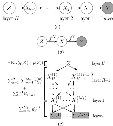
Our deep Gaussian process architecture corresponds to a graphical model with three kinds of nodes, illustrated in figure 1(a): the leaf nodes Y ∈ RN×D _{which are}

ob-served, the intermediate latent spacesXh ∈ RN×Qh, h=

1, ..., H−1, whereHis the number of hidden layers, and

the parent latent node Z = XH ∈ RN×QZ. The parent

node can be unobserved and potentially constrained with a prior of our choice (e.g. a dynamical prior), or could con-stitute the given inputs for a supervised learning task. For simplicity, here we focus on the unsupervised learning sce-nario. In this deep architecture, all intermediate nodesXh

act as inputs for the layer below (including the leaves) and as outputs for the layer above. For simplicity, consider a structure with only two hidden units, as the one depicted in figure 1(b). The generative process takes the form:

ynd=fdY(xn) +Ynd, d= 1, ..., D, xn∈ RQ

xnq=fqX(zn) +Xnq, q= 1, ..., Q, zn ∈ RQZ (4)

and the intermediate node is involved in two Gaussian pro-cesses,fY _andfX_{, playing the role of an input and an}

out-put respectively: fY _{∼ GP(0, k}Y_{(X,X)) and f}X _∼ GP(0, kX_{(Z,Z)). This structure can be naturally extended}

vertically (i.e. deeper hierarchies) or horizontally (i.e. seg-mentation of each layer into different partitions of the out-put space), as we will see later in the paper. However, it is already obvious how each layer adds a significant number of model parameters (Xh) as well as a regularization

chal-lenge, since the size of each latent layer is crucial but has to be a priori defined. For this reason, unlike Lawrence and Moore [2007], we seek to variationally marginalise out the whole latent space. Not only this will allow us to obtain an automatic Occam’s razor due to the Bayesian training, but also we will end up with a significantly lower number of model parameters, since the variational procedure only adds variational parameters. The first step to this approach is to define automatic relevance determination (ARD) co-variance functions for the GPs:

k(xi,xj) =σard2 e

−1 2

PQ

q=1wq(xi,q−xj,q)2_{. (5)}

This covariance function assumes a different weight wq

zero, thus helping towards automatically finding the struc-ture of complex models. However, the nonlinearities intro-duced by this covariance function make the Bayesian treat-ment of this model challenging. Nevertheless, following recent non-standard variational inference methods we can define analytically an approximate Bayesian training pro-cedure, as will be explained in the next section.

2.3 Bayesian Training

A Bayesian training procedure requires optimisation of the model evidence:

logp(Y) = log

Z

X,Z

p(Y|X)p(X|Z)p(Z). (6)

When prior information is available regarding the observed data (e.g. their dynamical nature is known a priori), the prior distribution on the parent latent node can be selected so as to constrain the whole latent space through propaga-tion of the prior density through the cascade. Here we take the general case wherep(Z) = N(Z|0, I). However, the integral of equation (6) is intractable due to the nonlinear way in whichXandZare treated through the GP priors

fY andfX. As a first step, we apply Jensen’s inequality to find a variational lower boundFv ≤logp(Y), with

Fv=

Z

X,Z,FY_,FX

Qlogp(Y,F

Y_,FX_,X,Z)

Q , (7)

where we introduced a variational distributionQ, the form of which will be defined later on. By noticing that the joint distribution appearing above can be expanded in the form

p(Y,FY,FX,X,Z) =

p(Y|FY)p(FY|X)p(X|FX)p(FX|Z)p(Z), (8)

we see that the integral of equation (7) is still intractable be-causeXandZstill appear nonlinearly in thep(FY_|X)and

p(FX_{|Z)terms respectively. A key result of [Titsias and}

Lawrence, 2010] is that expanding the probability space of the GP priorp(F|X)with extra variables allows for priors on the latent space to be propagated through the nonlinear mapping f. More precisely, we augment the probability space of equation (3) withKauxiliary pseudo-inputsX˜ ∈ RK×Q_{andZ˜ ∈ R}K×QZ_{that correspond to a collection of} function valuesUY ∈ RK×D_andUX _{∈ R}K×Q

respec-tively5. Following this approach, we obtain the augmented probability space:p(Y,FY_,FX_,X,Z,UY_,UX_{,X˜,Z˜) =}

p(Y|FY)p(FY|UY,X)p(UY|X˜)

·p(X|FX)p(FX|UX,Z)p(UX|X˜)p(Z) (9) The pseudo-inputsX˜ andZ˜ are known asinducing points, and will be dropped from our expressions from now on, for

5

The number of inducing points,K, does not need to be the same for every GP of the overall deep structure.

clarity. Note that FY andUY are draws from the same GP so that p(UY)and p(FY|UY,X) are also Gaussian distributions (and similarly forp(UX_{), p(F}X_|UX_,Z)).

We are now able to define a variational distribution Q

which, when combined with the new expressions for the augmented GP priors, results in a tractable variational bound. Specifically, we have:

Q=p(FY|UY,X)q(UY)q(X)

·p(FX|UX,Z)q(UX)q(Z). (10)

We select q(UY) andq(UX) to be free-form variational distributions, whileq(X)andq(Z)are chosen to be Gaus-sian, factorised with respect to dimensions:

q(X) =

Q Y

q=1

N(µX_q ,SX_q ), q(Z) =

QZ

Y

q=1

N(µZ_q,SZ_q). (11)

By substituting equation (10) back to (7) while also re-placing the original joint distribution with its augmented version in equation (9), we see that the “difficult” terms

p(FY_|UY_{,X) andp(F}X_|UX_{,Z) cancel out in the}

frac-tion, leaving a quantity that can be computed analytically:

Fv=

Z

Qlogp(Y|F

Y_)p(UY_)p(X|FX_)p(UX_)p(Z)

Q0 ,

(12) whereQ0 _{= q(U}Y_)q(X)q(UX_{)q(Z)and the above}

inte-gration is with respect to{X,Z,FY_,FX_,UY_,UX_{}. More}

specifically, we can break the logarithm in equation (12) by grouping the variables of the fraction in such a way that the bound can be written as:

Fv =gY +rX+Hq(X)−KL(q(Z)kp(Z)) (13)

whereHrepresents the entropy with respect to a distribu-tion, KL denotes the Kullback – Leibler divergence and, usingh·ito denote expectations,

gY =g(Y,FY,UY,X)

=Dlogp(Y|FY) + log_qp(₍U_UYY)₎

E

p(FY_|UY_,X)q(UY_)q(X)

rX =r(X,FX,UX,Z)

=Dlogp(X|FX) + log_qp(₍U_UXX)₎

E

p(FX_|UX_,Z)q(UX_)q(X)q(Z) (14)

Both termsgY andrX involve known Gaussian densities

and are, thus, tractable. The gY term is only associated

a quantity of the formYYT. Further, as can be seen from the above equations, the functionr(·)is similar tog(·)but it requires expectations with respect to densities of all of the variables involved (i.e. with respect to all function inputs). Therefore,rXwill involveX(the outputs of the top layer)

in a term

XXT q(X)=

PQ q=1

h

µX

q µXq

T

+SX

q i

.

3

Extending the hierarchy

Although the main calculations were demonstrated in a simple hierarchy, it is easy to extend the model ver-tically, i.e. by adding more hidden layers, or horizon-tally, i.e. by considering conditional independencies of the latent variables belonging to the same layer. The first case only requires adding more rX functions to the

variational bound, i.e. instead of a single rX term we

will now have the sum: PH_h=1−1rXh, where rXh =

r(Xh,FXh,UXh,Xh+1), XH =Z.

Now consider the horizontal expansion scenario and as-sume that we wish to break the single latent space Xh,

of layerh, toMh conditionally independent subsets. As

long as the variational distributionq(Xh)of equation (11)

is chosen to be factorised in a consistent way, this is fea-sible by just breaking the original rXh term of equation (14) into the sum PMh

m=1r (m)

Xh. This follows just from the fact that, due to the independence assumption, it holds that logp(Xh|Xh+1) =

PMh

m=1logp(X (m)

h |Xh+1).

No-tice that the same principle can also be applied to the leaves by breaking thegY term of the bound. This scenario arises

when, for example we are presented with multiple different output spaces which, however, we believe they have some commonality. For example, when the observed data are coming from a video and an audio recording of the same event. Given the above, the variational bound for the most general version of the model takes the form:

Fv =

MY

X

m=1 g_Y(m)+

H−1

X

h=1

Mh

X

m=1 r(_Xm)

h +

H−1

X

h=1

Hq(Xh)

−KL(q(Z)kp(Z)). (15) Figure 1(c) shows the association of this objective func-tion’s terms with each layer of the hierarchy. Recall that eachr(_Xm)

h andg

(m)

Y term is associated with a different GP

and, thus, is coming with its own set of automatic relevance determination (ARD) weights (described in equation (5)).

3.1 Deep multiple-output Gaussian processes

The particular way of extending the hierarchies horizon-tally, as presented above, can be seen as a means of per-forming unsupervised multiple-output GP learning. This only requires assigning a differentgY term (and, thus,

as-sociated ARD weights) to each vectoryd, wheredindexes

the output dimensions. After training our model, we hope

that the columns ofYthat encode similar information will be assigned relevance weight vectors that are also similar. This idea can be extended to all levels of the hierarchy, thus obtaining a fully factorised deep GP model.

This special case of our model makes the connection be-tween our model’s structure and neural network architec-tures more obvious: the ARD parameters play a role similar to the weights of neural networks, while the latent variables play the role of neurons which learn hierarchies of features.

...

(a)

(b)

(c)

Figure 1: Different representations of the Deep GP model: (a) shows the general architecture with a cascade ofH hid-den layers, (b) depicts a simplification of a two hidhid-den layer hierarchy also demonstrating the corresponding GP map-pings and (c) illustrates the most general case where the leaves and all intermediate nodes are allowed to form con-ditionally independent groups. The terms of the objective (15) corresponding to each layer are included on the left.

3.2 Parameters and complexity

In all graphical variants shown in figure 1, every arrow rep-resents a generative procedure with a GP prior, correspond-ing to a set of parameters {X˜,θ, σ}. Each layer of la-tent variables corresponds to a variational distributionq(X)

which is associated with a set of variational means and covariances, as shown in equation (11). The parent node can have the same form as equation (11) or can be con-strained with a more informative prior which would couple the points ofq(Z). For example, a dynamical prior would introduce Q× N2 _{parameters which can, nevertheless,}

be reparametrized using less variables [Damianou et al., 2011]. However, as is evident from equations (10) and (12), the inducing points and the parameters ofq(X)and

Therefore, adding more layers to the hierarchy does not introduce many more model parameters. Moreover, as in common sparse methods for Gaussian processes [Titsias, 2009], the complexity of each generative GP mapping is reduced from the typicalO(N3_{)toO(N M}2_).

4

Demonstration

In this section we demonstrate the deep GP model in toy and real-world data sets. For all experiments, the model is initialised by performing dimensionality reduction in the observations to obtain the first hidden layer and then re-peating this process greedily for the next layers. To obtain the stacked initial spaces we experimented with PCA and the Bayesian GP-LVM, but the end result did not vary sig-nificantly. Note that the usual process in deep learning is to seek a dimensional expansion, particularly in the lower layers. In deep GP models, such an expansiondoesoccur between the latent layers because there is an infinite basis layer associated with the GP between each latent layer.

4.1 Toy Data

We first test our model on toy data, created by sampling from a three-level stack of GPs. Figure 2 (a) depicts the true hierarchy: from the top latent layer two intermediate latent signals are generated. These, in turn, together generate10 -dimensional observations (not depicted) through sampling of another GP. These observations are then used to train the following models: a deep GP, a simple stacked Isomap [Tenenbaum et al., 2000] and a stacked PCA method, the results of which are shown in figures 2 (b, c, d) respec-tively. From these models, only the deep GP marginalises the latent spaces and, in contrast to the other two, it is not given any information about the dimensionality of each true signal in the hierarchy; instead, this is learnt automatically through ARD. As can be seen in figure 2, the deep GP finds the correct dimensionality for each hidden layer, but it also discovers latent signals which are closer to the real ones. This result is encouraging, as it indicates that the model can recover the ground truth when samples from it are taken, and gives confidence in the variational learning procedure.

(a) (b) (c) (d)

Figure 2: Attempts to reconstruct the real data (fig. (a)) with our model (b), stacked Isomap (c) and stacked PCA (d). Our model can also find the correct dimensionalities automatically.

We next tested our model on a toy regression problem. A deep regression problem is similar to the unsupervised

learning problem we have described, but in the uppermost layer we make observations of some set of inputs. For this simple example we created a toy data set by stacking two Gaussian processes as follows: the first Gaussian process employed a covariance function which was the sum of a linear and an quadratic exponential kernel and received as input an equally spaced vector of120points. We generated

1-dimensional samples from the first GP and used them as input for the second GP, which employed a quadratic expo-nential kernel. Finally, we generated10-dimensional sam-ples with the second GP, thus overall simulating a warped process. The final data set was created by simply ignor-ing the intermediate layer (the samples from the first GP) and presenting to the tested methods only the continuous equally spaced input given to the first GP and the output of the second GP. To make the data set more challenging, we randomly selected only 25datapoints for the training set and left the rest for the test set.

Figure 3 nicely illustrates the effects of sampling through two GP models, nonstationarity and long range correlations across the input space become prevalent. A data set of this form would be challenging for traditional approaches be-cause of these long range correlations. Another way of thinking of data like this is as a nonlinear warping of the input space to the GP. Because this type of deep GP only contains one hidden layer, it is identical to the model de-veloped by [Damianou et al., 2011] (where the input given at the top layer of their model was a time vector, but their code is trivially generalized). The additional contribution in this paper will be to provide a more complex deep hier-archy, but still learn the underlying representation correctly. To this end we applied a standard GP (1 layer less than the actual process that generated the data) and a deep GP with two hidden layers (1 layer more than the actual generating process). We repeated our experiment 10 times, each time obtaining different samples from the simulated warped pro-cess and different random training splits. Our results show that the deep GP predicted better the unseen data, as can be seen in figure 3(b). The results, therefore, suggest that our deep model can at the same time be flexible enough to model difficult data as well as robust, when modelling data that is less complex than that representable by the hierar-chy. We assign these characteristics to the Bayesian learn-ing approach that deals with capacity control automatically.

4.2 Modeling human motion

−2 −1 0 1 2 −2

−1 0 1 2 3

−2 −1 0 1 2

−4 −2 0 2 4

(a)

1 2 3 4 5 6 7 8 9 10

1 1.5 2 2.5 3 3.5 4

GP deepGP

experiment #

MSE

(b)

Figure 3: (a) shows the toy data created for the regression experiment. The top plot shows the (hidden) warping func-tion and bottom plot shows the final (observed) output. (b) shows the results obtained over each experiment repetition.

applied our method with a two-level hierarchy where the two observation sets were taken to be conditionally inde-pendent given their parent latent layer. In the layer closest to the data we associated each GP-LVM with a different set of ARD parameters, allowing the layer above to be used in different ways for each character. In this approach we are inspired by the shared GP-LVM structure of Damianou et al. [2012] which is designed to model loosely correlated data sets within the same model. The end result was that we obtained three optimised sets of ARD parameters: one for each modality of the bottom layer (fig. 4(b)), and one for the top node (fig. 4(c)). Our model discovered a com-mon subspace in the intermediate layer, since for dimen-sions2and6both ARD sets have a non-zero value. This is expected, as the two subjects perform very similar mo-tions with opposite direcmo-tions. The ARD weights are also a means of automatically selecting the dimensionality of each layer and subspace. This kind of modelling is impos-sible for a MAP method like [Lawrence and Moore, 2007] which requires the exact latent structure to be given a priori. The full latent space learned by the aforementioned MAP method is plotted in figure 5 (d,e,f), where fig. (d) corre-sponds to the top latent space and each of the other two encodes information for each of the two interacting sub-jects. Our method is not constrained to two dimensional spaces, so for comparison we plot two-dimensional projec-tions of the dominant dimensions of each subspace in figure 5 (a,b,c). The similarity of the latent spaces is obvious. In contrast to Lawrence and Moore [2007], we did not have to constrain the latent space with dynamics in order to obtain results of good quality.

Further, we can sample from these spaces to see what kind of information they encode. Indeed, we observed that the top layer generates outputs which correspond to different variations of the whole sequence, while when sampling from the first layer we obtain outputs which only differ in a small subset of the output dimensions, e.g. those

corre-sponding to the subject’s hand.

(a)

1 2 3 4 5 6 7 8 9 10

(b)

1 2 3 4 5 6 7 8 9 10

(c)

Figure 4: Figure (a) shows the deep GP model employed. Figure (b) shows the ARD weights for fY1 _(blue/wider bins) andfY2_{(red/thinner bins) and figure (c) those forf}X_.

(a) (b) (c) (d) (e) (f)

Figure 5: Left (a,b,c): projections of the latent spaces dis-covered by our model, Right (d,e,f): the full latent space learned for the model of Lawrence and Moore [2007].

4.3 Deep learning of digit images

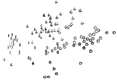
Our final experiment demonstrates the ability of our model to learn latent features of increasing abstraction and we demonstrate the usefulness of an analytic bound on the model evidence as a means of evaluating the quality of the model fit for different choices of the overall depth of the hierarchy. Many deep learning approaches are applied to large digit data sets such as MNIST. Our specific intention is to explore the utility of deep hierarchies when the digit data set is small. We subsampled a data set consisting of

50examples for each of the digits{0,1,6}taken from the USPS handwritten digit database. Each digit is represented as an image in16×16pixels. We experimented with deep GP models of depth ranging from1(equivalent to Bayesian GP-LVM) to 5 hidden layers and evaluated each model by measuring the nearest neighbour error in the latent fea-tures discovered in each hierarchy. We found that the lower bound on the model evidence increased with the number of layers as did the quality of the model in terms of nearest neighbour errors6_{. Indeed, the single-layer model made5} mistakes even though it automatically decided to use10 la-tent dimensions and the quality of the trained models was increasing with the number of hidden layers. Finally, only one point had a nearest neighbour of a different class in the

4−dimensional top level’s feature space of a model with depth5. A2Dprojection of this space is plotted in fig.7. The ARD weights for this model are depicted in fig. 6.

6

Our final goal is to demonstrate that, as we rise in the hier-archy, features of increasing abstraction are accounted for. To this end, we generated outputs by sampling from each hidden layer. The samples are shown in figure 8. There, it can be seen that the lower levels encode local features whereas the higher ones encode more abstract information.

1 2 3 4 5 6

12 34 5 67 89101112131415 layer 1

...

1 2 3 4 5 6 7 8 9 101112 layer 2

...

1 2 3 4 5 6 7 8 9 10 layer 3

...

1 2 3 4 5 6 7 8 layer 4

...

layer 5

...

Figure 6: The ARD weights of a deep GP with5hidden layers as learned for the digits experiment.

−5 0 5 10 15

x 10

Figure 7: The nearest neighbour class separation test on a deep GP model with depth5.

5

Discussion and future work

We have introduced a framework for efficient Bayesian training of hierarchical Gaussian process mappings. Our approach approximately marginalises out the latent space, thus allowing for automatic structure discovery in the erarchy. The method was able to successfully learn a hi-erarchy of features which describe natural human motion and the pixels of handwritten digits. Our variational lower bound selected a deep hierarchical representation for hand-written digits even though the data in our experiment was relatively scarce (150 data points). We gave persuasive ev-idence that deep GP models are powerful enough to en-code abstract information even for smaller data sets. Fur-ther exploration could include testing the model on oFur-ther inference tasks, such as class conditional density estima-tion to further validate the ideas. Our method can also be used to improve existing deep algorithms, something which

Figure 8: The first two rows (top-down) show outputs ob-tained when sampling from layers1and2respectively and encode very local features, e.g. explaining if a “0” has a closed circle or how big the circle of a “6” is. We found many more local features when we sampled from different dimensions. Conversely, when we sampled from the two dominant dimensions of the parent node (two rows in the bottom) we got much more varying outputs, i.e. the higher levels indeed encode much more abstract information.

we plan to further investigate by incorporating ideas from past approaches. Indeed, previous efforts to combine GPs with deep structures were successful at unsupervised pre-training [Erhan et al., 2010] or guiding [Snoek et al., 2012] of traditional deep models.

Although the experiments presented here considered only up to 5 layers in the hierarchy, the methodology is directly applicable to deeper architectures, with which we intend to experiment in the future. The marginalisation of the latent space allows for such an expansion with simultaneous reg-ularisation. The variational lower bound allows us to make a principled choice between models trained using different initializations and with different numbers of layers.

The deep hierarchy we have proposed can also be used with inputs governing the top layer of the hierarchy, leading to a powerful model for regression based on Gaussian pro-cesses, but which is not itself a Gaussian process. In the future, we wish to test this model for applications in multi-task learning (where intermediate layers could learn repre-sentations shared across the tasks) and in modelling nonsta-tionary data or data involving jumps. These are both areas where a single layer GP struggles.

A remaining challenge is to extend our methodologies to very large data sets. A very promising approach would be to apply stochastic variational inference[Hoffman et al., 2012]. In a recent workshop publication Hensman and Lawrence [2012] have shown that the standard variational GP and Bayesian GP-LVM can be made to fit within this formalism. The next step for deep GPs will be to incorpo-rate these large scale variational learning algorithms.

Acknowledgements

References

Y. Bengio. Learning Deep Architectures for AI. Found. Trends Mach. Learn., 2(1):1–127, Jan. 2009. ISSN 1935-8237. doi: 10.1561/2200000006.

Y. Bengio, A. C. Courville, and P. Vincent. Unsupervised feature learning and deep learning: A review and new perspectives. CoRR, abs/1206.5538, 2012.

A. C. Damianou and N. D. Lawrence. Deep Gaussian pro-cesses.NIPS workshop on Deep Learning and Unsuper-vised Feature Learning (arXiv:1211.0358v1), 2012.

A. C. Damianou, M. Titsias, and N. D. Lawrence. Varia-tional Gaussian process dynamical systems. In J. Shawe-Taylor, R. Zemel, P. Bartlett, F. Pereira, and K. Wein-berger, editors,Advances in Neural Information Process-ing Systems 24, pages 2510–2518. 2011.

A. C. Damianou, C. H. Ek, M. K. Titsias, and N. D. Lawrence. Manifold relevance determination. In J. Langford and J. Pineau, editors, Proceedings of the International Conference in Machine Learning, vol-ume 29, San Francisco, CA, 2012. Morgan Kauffman.

N. Durrande, D. Ginsbourger, and O. Roustant. Additive kernels for Gaussian process modeling. ArXiv e-prints 1103.4023, 2011.

D. Erhan, Y. Bengio, A. Courville, P.-A. Manzagol, P. Vin-cent, and S. Bengio. Why does unsupervised pre-training help deep learning? J. Mach. Learn. Res., 11:625–660, Mar. 2010. ISSN 1532-4435.

M. G¨onen and E. Alpaydin. Multiple kernel learning algo-rithms. J. Mach. Learn. Res., 12:2211–2268, Jul 2011. ISSN 1532-4435.

J. Hensman and N. Lawrence. Gaussian processes for big data through stochastic variational inference. NIPS workshop on Big Learning, 2012.

G. Hinton. A Practical Guide to Training Restricted Boltz-mann Machines. Technical report, 2010.

G. E. Hinton. Training products of experts by maximiz-ing contrastive likelihood. Technical report, Tech. Rep., Gatsby Computational Neuroscience Unit, 1999.

G. E. Hinton and S. Osindero. A fast learning algorithm for deep belief nets.Neural Computation, 18:2006, 2006.

G. E. Hinton and R. R. Salakhutdinov. Reducing the di-mensionality of data with neural networks. Science, 303 (5786):504–507, 2006.

M. Hoffman, D. Blei, C. Wang, and J. Paisley. Stochastic variational inference.ArXiv e-prints 1206.7051, 2012.

N. D. Lawrence. Gaussian process latent variable models for visualisation of high dimensional data. InIn NIPS, page 2004, 2004.

N. D. Lawrence. Probabilistic non-linear principal compo-nent analysis with Gaussian process latent variable mod-els. Journal of Machine Learning Research, 6:1783– 1816, 11 2005.

N. D. Lawrence and A. J. Moore. Hierarchical Gaussian process latent variable models. In Z. Ghahramani, editor, Proceedings of the International Conference in Machine Learning, volume 24, pages 481–488. Omnipress, 2007. ISBN 1-59593-793-3.

R. M. Neal. Bayesian Learning for Neural Networks. Springer, 1996. Lecture Notes in Statistics 118.

C. E. Rasmussen and C. K. I. Williams. Gaussian Pro-cesses for Machine Learning. Cambridge, MA, 2006. ISBN 0-262-18253-X.

R. Salakhutdinov and I. Murray. On the quantitative analy-sis of deep belief networks. InProceedings of the Inter-national Conference on Machine Learning, volume 25, 2008.

E. Snelson, C. E. Rasmussen, and Z. Ghahramani. Warped Gaussian processes. In S. Thrun, L. Saul, and B. Sch¨olkopf, editors,Advances in Neural Information Processing Systems 16. MIT Press, Cambridge, MA, 2004.

J. Snoek, R. P. Adams, and H. Larochelle. On nonparamet-ric guidance for learning autoencoder representations. In Fifteenth International Conference on Artificial Intelli-gence and Statistics (AISTATS), 2012.

J. B. Tenenbaum, V. de Silva, and J. C. Langford. A global geometric framework for nonlinear dimensionality re-duction. Science, 290(5500):2319–2323, 2000. doi: 10.1126/science.290.5500.2319.

J. B. Tenenbaum, C. Kemp, and P. Shafto. Theory-based bayesian models of inductive learning and reasoning. In Trends in Cognitive Sciences, pages 309–318, 2006.

M. Titsias. Variational learning of inducing variables in sparse Gaussian processes. JMLR W&CP, 5:567–574, 2009.

M. K. Titsias and N. D. Lawrence. Bayesian Gaussian pro-cess latent variable model. In Y. W. Teh and D. M. Tit-terington, editors,Proceedings of the Thirteenth Interna-tional Workshop on Artificial Intelligence and Statistics, volume 9, pages 844–851, Chia Laguna Resort, Sardinia, Italy, 13-16 May 2010. JMLR W&CP 9.