Energy efficient geographic routing robust against location errors

(1)

This is a repository copy of

Energy efficient geographic routing robust against location

errors

.

White Rose Research Online URL for this paper:

http://eprints.whiterose.ac.uk/82375/

Version: Accepted Version

Article:

Popescu, AM, Salman, N and Kemp, AH (2014) Energy efficient geographic routing robust

against location errors. IEEE Sensors Journal, 14 (6). 1944 - 1951. ISSN 1530-437X

https://doi.org/10.1109/JSEN.2014.2305832

[email protected] https://eprints.whiterose.ac.uk/

Reuse

Unless indicated otherwise, fulltext items are protected by copyright with all rights reserved. The copyright exception in section 29 of the Copyright, Designs and Patents Act 1988 allows the making of a single copy solely for the purpose of non-commercial research or private study within the limits of fair dealing. The publisher or other rights-holder may allow further reproduction and re-use of this version - refer to the White Rose Research Online record for this item. Where records identify the publisher as the copyright holder, users can verify any specific terms of use on the publisher’s website.

Takedown

If you consider content in White Rose Research Online to be in breach of UK law, please notify us by

(2)

Energy Efficient Geographic Routing Robust

Against Location Errors

Ana Maria Popescu, Naveed Salman, Andrew H. Kemp,

School of Electronic and Electrical Engineering, University of Leeds, UK, LS29JT

{elamp, elns, a.h.kemp}@leeds.ac.uk

Abstract—Realistic geographic routing algorithms need to ensure quality of services in wireless sensor network (WSN) applications whilst being resilient to the inherent localization errors of positioning algorithms. A number of solutions robust against location errors have been proposed in the literature and their design focuses either on a high throughput [1], [2] or on a balanced energy consumption [3], [4]. Ideally both aspects need to be addressed by the same algorithm, but in most cases the proposed routing techniques compromise between the two. The present work aims to minimize such a tradeoff and to facilitate a higher packet delivery ratio (PDR) than similar geographic routing techniques, while still being energy efficient. This is achieved through a novel proposal entitled energy conditioned mean square error algorithm (ECMSE) which, similarly to the forwarding method in [5], makes use of statistical assumptions of Gaussianly distributed location error and Ricianly distributed distances between sensor nodes. In addition it makes use of an energy efficient feature proposed by [3], which includes information about the energy cost of the forwarding decision. By using a location-error-resilient & distance-based power metric, the ECMSE provides an improved performance in realistic simulations in comparison with other error-coping algorithms.

Index Terms—geographic routing algorithm, energy efficiency, resilience to location errors, wireless sensor networks

I. INTRODUCTION

Wireless sensor network (WSN) technology is indisputably of interest to all branches of the industry, in the military, industrial, home automation and health fields [6], [7], [8], [9]. WSNs are now being used in applications of various scale which require sensing and monitoring equipment [10], [11]. They consist in spatially distributed autonomous sensor-equipped devices (referred to as sensor nodes), which collab-orate to communicate sensed data from the physical environ-ment [6]. Aside from sensing network events, many wireless sensor nodes are capable of locating themselves as well as other nodes. Local positioning systems are a preferred alter-native to the expensive, power-consuming global positioning system (GPS) devices [12], but although more cost-effective, the local positioning process is inherently erroneous and can affect network communication severely [13], [14].

The quality of service (QoS) requirements in WSNs are well known to be more stringent from those of ad-hoc networks. WSN dedicated forwarding algorithms need to ensure efficient data communication between hundreds of randomly deployed sensor devices with limited power supply and imperfect posi-tioning information. Geographic routing has often been seen as a promising forwarding technique which can optimally address

key WSN problems [7], [8], [9]. Although the advantages of this type of routing are many (it is a stateless, localized method, suitable for large scale networks), position-based routing needs to consider realistic assumptions and it thus needs to cope with the erroneous location information at sensor level [1], [4], [14], [15], [16], while minimizing the energy expenses of the devices as well [4], [16].

Routing strategies proposed in the literature use different design approaches, either optimizing the throughput [1], [2] or the energy consumption [3], [4]. For this, they employ various metrics based on distance and power costs. [5] analyzes geographic routing algorithms resilient to location errors by comparing their basic forwarding methods on similar grounds. The compared techniques in [5] are designed to use either the Rician expectation, the Rician variance or the mean square error (MSE). The proposed algorithm in [5], the conditioned mean square error ratio (CMSER) algorithm uses a distance-based metric. It was therefore necessary for the other algo-rithms considered in [5], meaning for the least expected dis-tance algorithm (LED) [4] and for the most expected progress (MEP) [2], to undergo modifications and to use distance-based metrics as well. However, the LED protocol, as proposed in [4], was originally designed on a hybrid metric encompassing power costs as well. The routing performance of LED is improved through the selection of the forwarding sensor node most proximal to an energy-optimal forwarding position. The calculation of such a position was first proposed in [3] and its purpose was that of making the routing process more energy efficient, rather than increasing the packet delivery ratio (PDR). The work herewith considers a similar energy-optimal forwarding choice in the case of the error-robust CMSER algorithm and proposes the energy conditioned mean square error algorithm (ECMSE) as an alternative with increased performance in comparison with CMSER or LED.

The main contributions of this paper are listed as follows: - Investigations are made considering realistic network aspects: a random node deployment, the existence of location errors of a different magnitude for each sensor node, the existence of multiple sensed events (and therefore of more traffic sources) and the use of the automatic repeat request (ARQ) mechanism, which is sometimes avoided in studies for simplification purposes.

(3)

- The analytical and simulation based comparison of LED and CMSER, two of the most recent location error-coping geographic routing solutions in the literature, with the new algorithm ECMSE, reveals the differences between the tech-niques for specific scenarios.

The manuscript is structured as follows. Section 2 presents related work on geographic routing robust against location errors, algorithms which are relevant for a better understanding of the current forwarding proposal. Section 3 introduces the assumed mathematical location error model. Section 4 explains the novel routing algorithm, ECMSE, and section 5 evaluates its behavior in a comparative manner in multiple scenarios mainly categorized as belonging to two different cases, with and without the use of a reception acknowledgment. Section 6 presents the conclusions.

II. RELATED WORK

Position-based algorithms face numerous design challenges which are sometimes neglected in novel protocol propositions. Geographic routing solutions require mathematical model-ing based on as many real-life challenges as possible [17], [18]; they need to rely on simple procedures which require little memory and few processing capabilities, need to be throughput-efficient, energy-optimal and have to consider re-alistic communication problems caused by noisy transmission environments and inaccurate location knowledge. Naturally, researchers have focused only on some of these aspects at times, neglecting others or making simplifying assumptions which enable mathematical theorisation.

Initial geographic routing studies avoid the inaccurate lo-calization issue and mainly focus on methods of forwarding which would improve the packet delivery or the power con-sumption. As an example of basic, distance-based geographic routing technique, with no error-coping capabilities, the most forward within range (MFR) [19] selects from the available forwarding candidates of a given sensor node based on its transmission range R and then forwards the data based on the distance between the neighbors and the destination D. The choice will be to send the information to the neighbor with the largest distance dij, assumed accurately known,

because this decision would ensure the shortest routing path. Considering for simplification the assumption of the unit disk model and the fixed transmission range, this would be the most energy efficient choice. However, in reality, the coordinates of the sensor nodes are not known with accuracy, nor is the transmission range model similar to a perfect disk. The performance of the MFR in a real-life application will not be the same as theoretically evaluated. Another example of a geographic routing technique, this time considering a power-aware metric and adjustable transmission range, is presented in [3]. The power aware algorithm however does not include inaccurate localization. In [1] more progress is made and it is pointed out that when a fixed transmission radius is used, a distance-based choice can be influenced by inaccurate localization and the selected furthest sensor node may also be the one nearest to the edge of R. As all decisions are made using estimated distances, the error magnitude can lead

to faulty routing decisions, transmission failure and consequent power wastage.

To avoid the energy losses incurred by data forwarding under erroneous positioning circumstances, the forwarding process can make use of a statistical error characteristic associated with the measured location of each sensor node [1], [2], [4], [5]. Algorithms such as LED [4] and the CMSER [5] improve their routing decisions by using the mean and error variance of the sensor devices; this statistical information, together with their coordinates, is communicated to them by the anchor nodes (devices with increased capabilities of sensing and processing which also perform localization)[12]. The additional data requires extra device memory, but aids in coping with location errors. With both algorithms, because the accurate locations are unknown and the actual distances are not available, the calculations are made using the estimated coordinates and distances instead. In both cases, the selected sensor node aims to offer a balance between the shortest distance toD and the smallest error characteristic.

III. ERROR MODEL

Early geographic routing studies assumed a simplistic ran-dom uniform error model [20], [16]. The assumption of a normally distributed location error was later considered more realistic and was employed in [1], [2], [4], [5], [15]. Also, the novel proposed algorithms in these references were aimed at efficiently coping with the Gaussian location errors. In the current work, location errors are considered independent normal random variables (RVs) and it is assumed that the error variance of each sensor node is different, but equal on the x

andy axes. Consequently, the accurate distance dij between

two devicesi andj is:

dij=

q

(xi−xj)

2

+ (yi−yj)

2

. (1)

The estimated distance dˆij is a normal RV with non-zero

mean (see Eq. 2)

ˆ

dij=

q

(ˆxi−xˆj)

2

+ (ˆyi−yˆj)

2

. (2)

The probability density function of dˆij follows a Rice

distribution [21],

fdˆij

= dˆij

σ2

ij

!

exp



−

ˆ

dij

2

+d2

ij

2σ2

ij



I0

ˆ

dijdij

σ2

ij

!

, (3)

where I0 is the modified Bessel function of the first kind

and order zero and σij is the scale parameter of the Rician

distribution:

σij =

q σ2

i +σ

2

j (4)

The mean (expectation) of the estimated distancedˆij is

Edˆij

=σij

r π

2L12 −

d2

ij

2σ2

ij

!

(4)

whereL1

2(x)denotes the Laguerre polynomial. The variance

of the estimated distancedˆij is

V ardˆij

= 2σ2

ij+d

2 ij− πσ2 ij 2 ! L2 1 2 − d 2 ij

2σ2

ij

!

. (6)

IV. THEECMSEALGORITHM

While LED forwards to the sensor node with the smallest expectation and uses Eq. 5, CMSER makes use of the mean square error (MSE) value associated with each neighbor device and computes a ratio (MSER) associated with each forwarding candidate:

M SERij =

Edˆij−dij

2

ˆ

dij

. (7)

The CMSER routing selection is then refined by considering that the squared difference between R and the estimated distance to the neighbor should be greater than the variance of the erroneous distance:

R−dˆij

2

> V ardˆij

. (8)

The scope of LED is however different from that of CMSER. It aims to preserve the power saving features of geographic forwarding, while still coping with location errors. It is stated in [4] that whichever approach the position-based routing may have, either to optimize the energy spent per hop or for the overall chosen path, the energy-optimal forwarding position is the same. LED determines this theoretical optimum and subsequently chooses as the next hop the neighbor whose estimated position is closest to it. The algorithm strategically incorporates location error into the forwarding objective func-tion. It is assumed that the estimated coordinates of each sensor node are affected by a Gaussian error of a given variance. As a consequence the erroneous distances between sensor nodes are random variables characterized by the Rice distribution. LED calculates the expectation of the considered distances and chooses the sensor node with the minimum expectation.

A general energy model per bit is presented in [22] and assumes that the total energy consumed per bit at the physical layer of a sensor device is the sum of the energy dissipated for the transmission (etx) and for the reception (erx) of

that bit, et = etx +erx. The energy consumption of the

transmission process consists of the energy spent on the radio electronics and that spent on the amplification of the signal. Therefore et=etx−elec+etx−amp+erx−elec. A simplifying

assumption is that the energy spent to operate the radio electronics is equal for both the transmission and the reception,

etx−elec =erx−elec =eelec, so et =etx−amp+ 2eelec. The

energy spent on the amplification can be further expressed as

etx₋amp = βdα, where α is the path loss index and β is

a constant [Joule/bit/mα_{]. Thus, the total energy consumed}

per bit can be written as:

et=βdα+c, (9)

where c = 2∗eelec. The expression changes for free space

or multipath, but for simplicity free space is the only case

considered here. The distance between the sensor nodei and the theoretical energy optimal positionM is calculated as in [3] or [4]:

diM = α

r _c

(β(1−21₋α₎₎. (10)

The energy-optimal position M is located on the line con-necting the currently transmitting sensor node i and the destination D. Using this information, the slope m of the line can be calculated with (yi −yD) = m(xi −xD). Its

value is the same for all the points on the line, including for M, so the coordinates xM and yM are found using the

following system of two equations: the point-slope formula for

(yi−yM) =m(xi−xM) and the equation of the Euclidean

distance diM =

p

(xi−xM)2+ (yi−yM)2 , where diM

value is obtained with Eq. 10 and m, xi, yi are known.

Depending on where M is found in reference to the sensor node i (on its left or right side): xM = xi± √diM

1+m2 and

yM =yi±√mdiM 1+m2.

With the known coordinates of M, LED can calculate the mean (expectation) of the measured distancedˆjM betweenM

and the neighborsj of sensor node iusing Eq. 5 and selects the option closest toM. The forwarding is made based on the objective function of LED, which minimizes the expectation:

Fj = arg min

EdˆjM

. (11)

In [5], to be able to compare the routing performance from a similar point of view, instead of using the LED algorithm for comparison, a basic form of it was employed. It forwarded based on the maximum Edˆij

used to determine the Fj

closest to D, instead ofEdˆjM

used by LED to determine the Fj closest to an energy-optimal forwarding position M.

The basic forwarding method of LED relays similarly to MFR, considering the notion of maximum advance to D, and its objective function is:

Fj= arg max

Edˆij

. (12)

The novel solution proposed here is the energy conditioned mean square error algorithm (ECMSE). It adopts the theoret-ical energy optimal pointM, as used in [4]. Because its aim is to select the neighbor j with the smallest error, instead of using the MSER in Eq. 7, the algorithm minimizes just the MSE in Eq. 13,

M SEij =E

ˆ

dij

2

−2dijE

ˆ

dij

+d2

ij, (13)

whereEdˆij

2

is calculated as in [5] to be:

Edˆij

2

= 2σ2

i + 2σ

2

j+x

2

i +x

2

j+y

2

i +y

2

j−2xixj−2yiyj.

(14) It then makes its choice considering the option closest toM, so minimizing the distance between j andM. The objective function of ECMSE will therefore be:

Fj= arg min

M SEij∗dˆjM

(5)

ECMSE also makes use of the condition in Eq. 8, just like CMSER. The ECMSE algorithm can be formalized as follows in Alg. 1.

Algorithm 1 ECMSE

ECMSE (S, D)

i:=S

do

if D is a neighbor ofi

then send packet toD;

else

calculate optimal position M;

forj:= 1to J (J is the number of neighbors ofi) calculateM SEij anddˆjM;

if(j minimizesM SEij∗dˆjM) and

(j ensuresR−dˆij

2

> V ardˆij

)

thensend packet to j;

j:=i;

end

until j=D;

V. SIMULATION AND RESULTS

As CMSER has already been proven to be robust against location errors and to have a better throughput than that of the modified version of LED [5], the performance of ECMSE is the one which remains to be studied. Hence, the original LED, CMSER and ECMSE are first compared based on the throughput. Then, the energy consumption is studied, considering the realistic case in which the routing benefits from transmission acknowledgment. The energy spent in the routing process is influenced by the number of successful transmissions and by the efforts of resending the data to achieve this. Both aspects are analyzed for networks which are dense enough to ensure the highest PDR possible (always of almost 100%).

The sensor devices are erroneously localized with σ2

i,

σ2

j∈[0, σ

2

max]. The MATLAB simulation parameters are listed

in Table I. Sensor nodes are randomly distributed and several scenarios are studied, as described in Table II, where SE

random sensing events take place. Performance is studied for different network densities (the number of nodesN is varied), for different values of the maximum standard deviation of errors (σmax) or different R. A fixed transmission power is

used and the probability of correctly receiving any packet within R is considered 1, and 0 outside R. Each scenario con-sists of a sensor node distribution with accurate coordinates, where packet forwarding is made with MFR (MFR-NoError). During the same simulation, a number ofη distributions with inaccurate locations (η being the number of trials/iterations) takes place, where the errors have been modeled as in section 3. The packet forwarding is made by the MFR-WithError, LED, CMSER and ECMSE. The figures are obtained through averaging overη.

While the first three scenarios listed in Table II do not consider the use of any reception acknowledgment (ACK) and are marked in the table with N (No), in the fourth and

Table I

SIMULATION PARAMETERS

Simulator parameters (unit) Symbol Value

Transmission power (W) Pt 1.778 Distance of reference (m) d0 1

Path loss exponent α 3

Packet size (bits) psize 1024 Data rate (Kbits/s) dr 250 Number of packets/source pkts 1 Energy spent on the radio electronics (nJ/bit) eelec 50

Energy spent on transmission(J/bit) etx 2.5e-07 Energy spent for reception (J/bit) erx 1.5e-0.7

Constant (pJ/bit/m2

) β 100

Network side length (m) l 50

fifth ones the performance of the algorithms is analyzed for a ’best effort’ type of packet forwarding and are marked with Y (Yes). The use of the ACK messages sent by receiving sensor nodes increases the overhead of the network and influences the energy consumption mainly through the number of necessary retransmissions. Each forwarding sensor node tries to transmit to each of its detected neighbors, until either the packet is received or all forwarding options are exhausted. Routing with reception confirmation does not imply a guaranteed delivery of the sent data packets; it is only a way of improving the reception chances and finding the path toD when one exists. Hence, when the networks have a good node density, the PDR is always above 98% for all algorithms. For sparse networks, the PDR changes depending on sensor node topology and magnitude of the location errors.

The simulations using a realistic acknowledgment assump-tion have the purpose of facilitating the energy consumpassump-tion analysis of the algorithms by maintaining the same PDR for all algorithms. The differences in the design of the algorithms results in a different number of hops for the received packets, of retransmissions at each sensor node and consequently in different levels of energy losses and network lifetime for each. The total energy consumed in a network (Etotal) represents the

sum of the energy spent on all packet transmissions (including the re-transmissions when no ACK is received) and of the energy spent receiving. The total number of transmissions is T rN o and the energy spent on receiving is calculated based on the average number of hops in the path of each received packet, HopN o. Thus Etotal = Etrans +Ercv,

whereEtrans=T rN o∗etx∗pkts∗SE∗psize andErcv =

HopN o∗erx∗pkts∗SE∗psize. For simplicity, the results

obtained for scenarios 4 and 5 and presented in parallel - all their parameters are the same, except for the total number of transmitted data packets in the network.

Table II SIMULATION SCENARIOS Scenario N R(m) σmax(m) (%

ofR)

η SE ACK

1 50-400 40 8 (20%) 100 10 N

2 200 10 1-25 (10-50%) 100 10 N

3 200 5-25 1 (20-4%) 100 10 N

(6)

Under all the scenarios, the PDR of the ECMSE algorithm is higher than that of CMSER or LED. In Fig. 1 the number of sensors is increased gradually from 50 to 400 devices. As expected LED has a better performance than CMSER, but its PDR is not as good as that of ECMSE, which uses the same distance-energy metric as LED. Because of the speed of the simulation, only 10 sensing events were chosen to take place in these networks, generating 10 traffic connections. If more were used, the PDR values would also be influenced.

50 100 150 200 250 300 350 400 0

10 20 30 40 50 60 70 80 90 100

Number of nodes

PDR [%] MFR−NoError

[image:6.612.332.539.113.261.2]

MFR−WithError CMSER LED ECMSE

Figure 1. Routing performance for scenario 1, with ECMSE

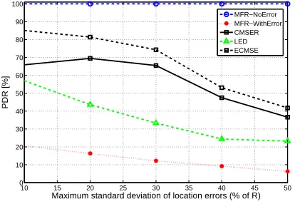
For Scenario 2, when increasing the location error, the PDR decreases considerably for all algorithms, as in Fig. 2. CMSER and ECMSE have a similar behavior, with a difference in PDR which shows the superiority of ECMSE. When σ is below 30% of R, the PDR is above 60% for CMSER and above 70% for ECMSE. So, if a tolerable amount of location error is associated with the case when σ is up to 10% ofR, then ECMSE is the most indicated choice for routing because it provides a PDR of 85%. Due to the reducedRin Scenario 2, LED maintains the PDR values under 60% and is constantly lower in delivery in comparison to CMSER and ECMSE.

10 15 20 25 30 35 40 45 50 0

10 20 30 40 50 60 70 80 90 100

Maximum standard deviation of location errors (% of R)

PDR [%]

[image:6.612.72.276.187.334.2]

MFR−NoError MFR−WithError CMSER LED ECMSE

However, Fig. 3 which considers an increase in R, while keeping the location error constant, reveals the change in behavior for the LED algorithm. While LED performs worse than CMSER for R ≤10, its PDR is similar to ECMSE for

larger values, reaching 90% values forR≥15. Nevertheless, ECMSE is preferred to LED because it performs better for small values ofR making it more energy efficient.

5 10 15 20 25

0 10 20 30 40 50 60 70 80 90 100

Transmission Range R

PDR [%]

[image:6.612.71.278.525.668.2]

The following results are obtained for the networks where the routing benefits from packet acknowledgment. For the two scenarios in Fig. 4 and Fig. 5, the hop count values are mainly influenced by the number and position of the sources in the network. In scenario 4 the one source sending packets has its erroneous location varied for each iteration, but the distance between it and D does not change considerably, being limited by the error variance. For scenario 5, the 50 different sources affect the number of hops of the received packets severely because the sending sensor nodes are located at different distances fromD. An average hop count will vary on the average distance between them andD, which does not coincide with the one in scenario 4.

For scenario 4, the average number of hops for the received packets in the network does not vary much from one algorithm to the next (being on average 2 or 3 hops). Also, as expected, LED provides shorter paths than CMSER and ECMSE, but this does not mean it is more energy efficient (as can be seen in Fig. 10 and Fig. 11). Naturally, the hop count decreases with the increase in sensor node density which contributes to the increase of the forwarding options, but none of the networks chooses a shorter path than the network with no location error. Between CMSER and ECMSE, the improved version of the algorithm provides visibly shorter routes.

For scenario 5, the figure reflects that ECMSE provides routing paths similar to the network with no location error, improving for the denser networks with more than 300 devices. LED however chooses even shorter paths to guarantee the same PDR. Although this can be seen as an advantage, the trade-off is a higher number of retransmissions which consume energy and whose numbers rise for denser networks. An overall analysis indicates that LED is also more suitable for sparser networks.

(7)

100 150 200 250 300 350 400 450 500 2

2.1 2.2 2.3 2.4 2.5 2.6 2.7 2.8

Number of nodes

Average number of hops per received packet

[image:7.612.64.268.70.216.2]

Figure 4. Average number of hops per received packet for scenario 4

100 150 200 250 300 350 400 450 500 4.5

5 5.5 6 6.5 7 7.5

Number of nodes

Average number of hops per received packet

[image:7.612.326.532.71.216.2]

Figure 5. Average number of hops per received packet for scenario 5

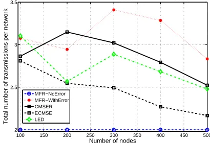
will make use of more retransmissions than CMSER and ECMSE. This expectation is confirmed in Fig. 6 and Fig. 7. The number of total transmissions depends on the number of retransmissions and on the number of hops of the received packets. Because the routing paths of the received packets for the CMSER algorithm are longer than any other, but its number of retransmissions are fewer than that of MFR or LED, the total number of transmissions situate it above LED and under MFR, as it can be seen in Fig. 8 and Fig. 9.

The energy costs are presented in Fig. 10 and Fig. 11. Sim-ulations show that ECMSE is energy efficient, while providing the same PDR as the rest of the algorithms. For Scenario 4, ECMSE is the most energy efficient being surpassed only by the network in which sensor nodes benefit from exact location knowledge. In this case, LED is the second most energy efficient algorithm, followed by CMSER whose longer routing paths cause more energy consumption. CMSER is slightly more wasteful due to error-aware decisions based only on a distance metric, without consideration for energy-optimal forwarding choices. For all the algorithms, the energy expenditure is reduced by increasing the network density. For Scenario 5, ECMSE, LED and the network with no location error have a similar energy consumption level, with a slight decrease for ECMSE when increasing the number of sensing devices in the network.

50 100 150 200 250 300 350 400 450 500 0

0.1 0.2 0.3 0.4 0.5 0.6 0.7 0.8

Number of nodes

Total number of retransmissions per network

[image:7.612.58.263.258.402.2]

Figure 6. Total number of retransmissions for scenario 4

100 150 200 250 300 350 400 450 500 0

50 100 150 200 250 300

Number of nodes

Total number of retransmissions per network

Figure 7. Total number of retransmissions for scenario 5

VI. CONCLUSIONS

All the simulated scenarios prove that ECMSE is an im-proved algorithm in terms of both PDR and overall energy consumption. The performance of ECMSE is conditioned by sensor network density, making it ideal for large scale scenar-ios. Under the same location error and energy constraints as other algorithms, ECMSE is an optimal routing candidate for

100 150 200 250 300 350 400 450 500 2

2.5 3 3.5

Number of nodes

Total number of transmissions per network

MFR−NoError MFR−WithError CMSER ECMSE LED

[image:7.612.318.523.266.409.2] [image:7.612.325.530.581.721.2]

(8)

100 150 200 250 300 350 400 450 500 250

300 350 400 450 500 550 600 650

Number of nodes

Total number of transmissions

[image:8.612.57.261.65.210.2]

Figure 9. Total number of transmissions for scenario 5

100 150 200 250 300 350 400 450 500 0.8

0.9 1 1.1 1.2 1.3x 10

−3

Number of nodes

Total Energy Consumption (Joules)

[image:8.612.63.270.253.399.2]

Figure 10. Total energy consumption for scenario 4

WSN applications in need of efficient, location error-coping geographic routing. It is a robust solution when sensor devices use low transmission power and has been proven energy efficient because of the number of required retransmissions for a best-effort routing scenario with reception acknowledgment. Even with slightly longer paths than LED, it performs better in terms of throughput (as seen when no ACK is used) and energy savings alike.

Although geographic routing solutions resilient to location

100 150 200 250 300 350 400 450 500 0.1

0.12 0.14 0.16 0.18 0.2 0.22

Number of nodes

Total Energy Consumption (Joules)

Figure 11. Total energy consumption for scenario 5

errors have been provided herewith, the current algorithms are not fully developed to the degree that a protocol or standard would be. Furthermore, the approaches of CMSER and ECMSE are based on the simplifying assumption that the location errors of each node are the same for the x and y

coordinates. This facilitates the statistical supposition that the distances between sensing devices are Ricianly distributed. Because the initial assumption is clearly not always true, it is believed to contribute to a less-realistic routing behavior. The impact of this theoretical presumption on the proposed algorithms should be explored in future work.

REFERENCES

[1] S. Kwon, N.B. Shroff, “Geographic routing in the presence of location errors”, Computer Networks, vol. 50, pp. 2902-2917, 2006

[2] R. Marin-Perez, P.M. Ruiz, “Effective Geographic Routing in Wireless Networks with Inaccurate Location Information”, In Proceedings of the 10th International conference on Ad-hoc, mobile, and wireless networks (ADHOC-NOW’11), Hannes Frey, Xu Li, and Stefan Ruehrup (Eds.). Springer-Verlag, Berlin, Heidelberg, pp. 1-14.

[3] Ivan Stojmenovic, Xu Lin, “Power-Aware Localized Routing in Wireless Networks”, IEEE Transactions Parallel Distributed Systems 12, 11, pp.1122-1133, Nov. 2001

[4] B. Peng, A.H. Kemp, “Energy-efficient geographic routing in the pres-ence of location errors”, Computer Networks, vol. 55, pp. 856-872, 2011 [5] A.M. Popescu, N. Salman, A.H. Kemp, “Geographic Routing Resilient to Location Errors”, IEEE Wireless Communications Letters, vol.2, no.2, pp.203-206, April 2013.

[6] I. F. Akyildiz, W. Su, Y. Sankarasubramaniam, E. Cayirci, “A survey on sensor networks”, IEEE Communication Magazine, vol. 40, no. 8, pp. 102–114, Aug. 2002

[7] K. Akkaya, M. Younis, “A survey on routing protocols for wireless sensor networks”, Ad Hoc Networks, vol. 3, pp. 325-349, 2005. [8] R.V. Biradar, V.C. Patil, S.R. Sawant, R.R. Mudholkar, “Classification

and Comparison of routing protocols in wireless sensor networks”, Special Issue on Ubiquitous Computing Security Systems, Vol. 4, pp. 325-349, July 2009.

[9] A. M. Popescu, I. G. Tudorache, A. H. Kemp, “Surveying Position Based Routing Protocols for Wireless Sensor and Ad-hoc Networks”, International Journal of Communication Networks and Information Security, Kohat University of Science and Technology (KUST), Pakistan, vol4, no. 1, 2012.

[10] J. Azevedo, F. Santos, “An empirical Propagation Model for Forest Environments at Tree Trunk Level”, IEEE Transactions on Antennas and Propagation, 59, pp. 2357-2367, 2011.

[11] C. Lochert, M. Mauve, H. FüSSler, “Geographic Routing in City Sce-narios”, ACM SIGMOBILE Mobile Computing and Communications Review, vol. 9, issue 1, , pp. 69-72, Jan. 2005.

[12] N. Salman, M. Ghogho, A.H. Kemp, “Optimized Low Complexity Sensor Node Positioning in Wireless Sensor Networks”, IEEE Sensors Journal, vol.14, no.1, pp.39-46, Jan. 2014.

[13] N. Patwari, A.O. Hero, III, M. Perkins, N.S. Correal, R. J. O’Dea, “Rela-tive location estimation in wireless sensor networks”, IEEE Transactions Signal Processing, vol. 51, no. 8, pp. 2137-2148, Aug. 2003. [14] Y. Kim, J.-J.Lee, A. Helmy, “Modeling and Analyzing the Impact of

Location Inconsistencies on Geographic Routing in Wireless Networks”, ACM SIGMOBILE Mobile Computing and Comm. Rev., vol. 8, no. 1, pp. 48-60, Jan. 2004.

[15] M. Witt, V. Turau, “The Impact of Location Errors on Geographic Routing in Sensor Networks”, Proceedings of the International Multi-Conference on Computing in the Global Information Technology ICCGI ’06, IEEE Computer Society, 2006.

[16] R.C. Shah, A. Wolisz, J.M. Rabaey, “On the performance of geograph-ical routing in the presence of localization errors”, IEEE International Conference on Communications, vol. 5, pp. 2979-2985, 2005. [17] Y. Kong, Y. Kwon, Y., J. Shin, G. Park, “Localization and dynamic

link detection for geographic routing in non-line-of-sight (NLOS) environments”, EURASIP Journal on Wireless Communications and Networking, 2011.

[image:8.612.54.260.580.725.2]

(9)

[19] H. Takagi, L. Kleinrock, “Optimal transmission range for randomly dis-tributed packet radio terminals”, IEEE Transactions on Communications 32 (3), pp.246-257, 1984.

[20] K. Seada, A. Helmy, R. Govindan, “On the effect of localization errors on geographic face routing in sensor networks”, In Proceedings of the 3rd International Symposium on Information processing in sensor networks (IPSN ’04), ACM, New York, NY, USA, pp.71-80, 2004. [21] K.S. Miller, “Multidimensional Gaussian Distributions”, John Wiley and

Sons, Inc., New York, London, Sydney, 1964

[22] W.B. Heinzelman, A.P. Chandrakasan, H. Balakrishnan, “An application-specific protocol architecture for wireless microsensor networks”, IEEE Transactions on Wireless Communications, vol.1, no.4, pp.660-670, Oct. 2002.

Ana Maria Popescu received her Engineering Diploma from the Faculty of Automation, Comput-ers and Electronics in Craiova, Romania, in 2008. She was then awarded a study scholarship at the Polytechnic Faculty of Mons, Belgium to conduct research in wireless sensor communication for home automation systems and vehicle monitoring. In 2009 she was accepted to pursue her PhD study at the University of Leeds, in the School of Electronic and Electrical Engineering, under the supervision of Dr. A.H. Kemp. Her research interests are in energy efficient wireless sensor networks (WSNs) and particularly in geographic routing algorithms and their quality of services (QoS). She has pulished several conference and journal papers in international journals such as the INTERNATIONAL JOURNAL OF COMMUNICATION NETWORKS AND INFORMATION SECURITY (IJCNIS), IET NETWORKS and IEEE COMMUNICATION LETTERS.

Naveed Salmanreceived his bachelor’s degree with Honours in Electrical and Electronics Engineering in 2007 from NWFP University of Engineering and Technology, Peshawar, Pakistan. In 2009 he received his Master’s degree with distinction from the Uni-versity of Leeds, UK. He also recently received his Ph.D. Degree from the University of Leeds, UK, in 2013. Naveed is the author of a number of journal and conference publications and is the recipient of the 2012 GW Carter best paper award from Leeds University. Naveed serves as a reviewer for several international journals and conferences including the IEEE TRANSACTIONS ON WIRELESS COMMUNICATIONS, IEEE TRANSACTIONS ON COM-MUNICATIONS, IEEE WIRELESS COMMUNICATIONS LETTERS and IEEE COMMUNICATIONS LETTERS.