Timebands
.
White Rose Research Online URL for this paper:
http://eprints.whiterose.ac.uk/94536/
Version: Submitted Version
Book Section:
Wei, Kun, Woodcock, Jim orcid.org/0000-0001-7955-2702 and Burns, Alan
orcid.org/0000-0001-5621-8816 (2012) Modelling Temporal Behaviour in Complex
Systems with Timebands. In: Hinchey, Mike and Coyle, Lorcan, (eds.) Conquering
Complexity. SPRINGER , London , pp. 277-307.
https://doi.org/10.1007/978-1-4471-2297-5_13
[email protected] https://eprints.whiterose.ac.uk/ Reuse
Items deposited in White Rose Research Online are protected by copyright, with all rights reserved unless indicated otherwise. They may be downloaded and/or printed for private study, or other acts as permitted by national copyright laws. The publisher or other rights holders may allow further reproduction and re-use of the full text version. This is indicated by the licence information on the White Rose Research Online record for the item.
Takedown
If you consider content in White Rose Research Online to be in breach of UK law, please notify us by
Modelling Temporal Behaviour in Complex
Systems with Timebands
Kun Wei, Jim Woodcock, and Alan Burns
13.1 Introduction
Complex real-time systems exhibit dynamic behaviours on many different time lev-els. For example, circuits have nanosecond speeds for computation in a component, whereas slower functional units may take seconds to achieve their goals; moreover, the involvement of human activities related to calendar units such as days, weeks, months and even years may take more time. To cope with a wide range of time scales, many approaches [10,23] have introduced time granularity, so that system specifications and requirements could be naturally described within the best suit-able time granularity. However, they usually transform or project all descriptions into the finest granularity in the end. This results in cumbersome formulae and fails to recognise the distinct role that time is taking in the structuring of the system. For example, it is unnecessary to measure the start of a meeting in a millisecond time scale. In fact, most people are usually tolerant of starting a meeting five min-utes early or late. Traditional approaches dealing with time granularity sacrifice the separation of concerns in the analysis of complex real-time systems.
To overcome the above weakness when traditional approaches model dynamic temporal behaviours of a system, Burns and Hayes [5] propose a timebands model in which a system is decomposed to reveal different behaviours in different time bands. Apart from defining time bands by granularities, a key aspect of the time-bands framework is thateventsare considered to be instantaneous in a band, and then in a finer band they can be mapped intoactivitiesthat have duration. For ex-ample, to express a statement thatevery month we have a meeting which lasts one hour, we model the meeting as an instantaneous event in a month band and subse-quently map it into an activity in an hour band. This clearly allows dynamic temporal behaviours to be partitioned, but not to be isolated from each other. The mapping
K. Wei (
)
Department of Computer Science, University of York, York, UK e-mail:[email protected]
M. Hinchey, L. Coyle (eds.),Conquering Complexity,
DOI10.1007/978-1-4471-2297-5_13, © Springer-Verlag London Limited 2012
between different bands leads to more distinct features. For example, precision is in-troduced to represent the measure of accuracy of events within a band; accordingly, events aresimultaneousonly if, when viewed from a finer band, their corresponding activities are within the precision. Activities may overlap even though their corre-sponding events in a coarser band are well-ordered. As a result, a formal model of the timebands framework is needed to allow consistency to be asserted between different temporal descriptions that are specified in different time bands.
The concept of time granularity has been well defined in the literature [8,16] and many approaches have focused on time granularity in different areas of com-puter science, such as temporal databases, data mining, formal specification and so on. General speaking, the basic idea of time granularity is to partition a universal time domain into differently-grained granules, and a granularity is a set of indexed granules, any one of which is a set of time instants. The choice for time domain is typically between continuous (dense) and discrete. We focus on developing a natural specification language which is able to describe the behaviour of a real-time system whose components engage in different time scales. In other words, we attempt to embed time granularity in a logical specification language. However, adding time granularity to a formalism may give rise to semantic issues like problems of assign-ing a proper meanassign-ing to statements with different time domains and of switchassign-ing from one domain to a coarser/finer one. So far, most work has been focused on embedding time granularity in temporal logic languages. For example, early explo-ration [10,23] consists of translation mechanisms that map a formula associated with different time constraints to the finest granularity. They [7] later revise the sim-ple approach by extending the basic logic language with contextual and projection operators, so that the enhanced semantics can express more general and complete properties. Subsequently, more work [9, 12] uses linear time logic to model and reason about time granularity.
For manipulating the unique feature of mapping events into activities, process algebra approaches are potential candidates for formalising the timebands model. However, there is little work on embedding time granularity in process algebra lan-guages, though there have been many papers [19,28,29] on timed process alge-bra approaches. To formalise the timebands model, we have proposed a new timed model of CSP, called timed CSP with the miracle (TCSPM), which is an extension to
timed CSP [28] but whose semantics is based onUnifying Theories of Programming
(UTP) [15]. This new model uses a complete lattice with respect to the implication order (or the reverse order of the refinement order), which is rather different from previous models such as the complete partial order of CSP [14,25,28]. The seman-tics of the timebands model is built uponTCSPM, fully applying the miracle (the top
element of the complete lattice) to express those brand-new features such as simul-taneous events and mappings. In this chapter, we use a mine pump example to show how naturally to verify different temporal properties using the timebands model at different time scales. The idea and informal description of the timebands framework has been given in [5], and the formal semantics of the framework is developed in this chapter.
The chapter is structured as follows. We begin with a brief introduction of
formalise the timebands model and how to formally express these distinct features. Then, by means of a rather complex example, we demonstrate how significantly the timebands model contributes to describing a complex real-time system with multi-ple time scales in Sect.13.4. Section13.5concludes this chapter.
13.2 Timed CSP with the Miracle
Recently, we have proposed a new timed model [32] ofCircus[26,33] which is a combination of CSP, Z [34] and the refinement calculus so as to define both data and behavioural aspects of a system. In fact, our timedCircusis a compact exten-sion ofCircusin that it inherits only the CSP part in order to reduce the difficulty of implementingCircusprograms in practice. Although it does not have the same capability of handling data as the originalCircuslanguage does, our timedCircus
preserves local variables for each process that still contains a considerable power to express the change of states. To formalise the timebands model, we further simplify timedCircustoTCSPM by adopting discrete time.
Simply speaking,TCSPM can also be considered an extension to Schneider’s
timed CSP [28], but its UTP-style semantics uses a complete lattice in the impli-cation ordering which is different from the complete partial order of timed CSP. With the application of the miracle (the top element of the model),TCSPM turns
out to be able to express some surprising behaviours which, moreover, cannot be described in timed CSP. Additionally,TCSPMviolates some axioms of the standard
failures-divergences model of CSP, e.g., traces are not prefix closed any more. In UTP, Hoare and He use the alphabetised relational calculus to give a denota-tional semantics that can explain a wide variety of programming paradigms. Hence, the alphabet of a processP inTCSPMconsists ofundashedvariables(a, b, . . .)and
dashedvariables(a′, x′, . . .). The former, written asinαP, stands for initial obser-vations, and the latter asoutαP for intermediate or final observations. The relation is then calledhomogeneousifoutαP=inαP′, whereinαP′ is simply obtained by putting a dash on all the variables ofinαP. Thus, an observation inTCSPM is a
tuple consisting oftr,ref,ok,wait,t,vand their dashed counterparts, in whichtr
andtr′are timed traces,ref andref′are refusals,okis a boolean variable expressing whether a process has started or not (ok′whether the process has terminated or not),
wait′denotes whether the process is in an intermediate state,tis the starting time of the observation (t′is the finishing time), andvandv′denote a set of local variables of the process.
A timed trace is a sequence of timed events which are pairs drawn fromZ+×,1 e.g., (1,pump.on), (3,pump.off) is a timed trace. A refusal is simply a set of events, other than a set of time events in timed CSP, since other variables can assist in representing enough information of when those events are refused. Theok and
waitobservations (and their dashed variables) describe whether a process is started
(or finished) in a stable state. Ifok′ is false, the process diverges. Ifok′is true, the state of the process depends on the value ofwait′. Ifwait′is true, the process is in an intermediate state, otherwise it successfully terminates. Similarly, the values of undashed variables represent the states of the process’s predecessor.
Except for the deadline and assignment operators, the syntax ofTCSPMis similar
to the one of timed CSP, as described by the following grammar:
P :: = ⊤R| ⊥R|SKIP|STOP|a→P |P1;P2|x:=Ae|g&P |
P1P2|P1⊓P2|P1|[A]|P2|P\A|WAITd|P1⊲ {d}P2|
P ◮d|P1△{a}P2|μX.P
13.2.1 Primitive Processes
The miracle⊤Ris the top element in the implication ordering, however it cannot be
executed since it expresses that a process has not started yet. Of course, an unstarted process satisfies any requirement. The bottom element⊥R is calledAbort which
can do absolutely anything. The processSTOPis deadlocked and its only behaviour is to allow time to elapse. The processSKIPsimply terminates immediately.
13.2.2 Sequential
The sequential compositionP1;P2 behaves as P1 until P1 terminates, and then
behaves asP2. In the meanwhile the final state ofP1is passed on as the initial state
ofP2. The prefix process a→P is able to execute the eventa (a∈) and then
behaves asP. This process can also be represented by a composition of a simple prefix andP itself, written as (a→SKIP);P. The process g&P has a boolean expressiong, which must be satisfied beforeP starts.
The notation(x:=Ae)represents that a process simply assigns the value of an
expressioneto a process variablex, and any other variable in the alphabetAremains unchanged. In practice, we often use a shorthand for the assignment operator. For example,P (x+1)is actually defined as (x:=x+1;P).
13.2.3 Choice
The processP1P2behaves either likeP1orP2, but the first event of which can
resolve the choice. Compared with this external choice, the internal choiceP1⊓P2
can also behave either likeP1or likeP2, but it is out of control of its environment.
finite indexing set such thatPi is defined for each i∈I, written as
i∈IPi. Theindexing external choice is also used to define the input operator. For example, ifcis a channel name of typeT andvis a particular value, the processc!v→P outputting
valong the channelcis equal toc.v→P. The inputting processc?x:T →P (x)
describes a process that is ready to accept any valuexof typeT, and it is defined as
x∈Tc.x→P (x).
13.2.4 Parallel
The processP1|[A]|P2 is the process where all events in the setAmust be
syn-chronised, and the events outsideAcan execute independently. The parallel process terminates only if bothP1andP2terminate, and it becomes divergent after either
one ofP1andP2does so. An interleaving of two processes,P1|||P2, executes each
part independently and is equivalent toP1|[ ∅ ]|P2.
13.2.5 Abstraction and Recursion
The hiding operatorP \Amakes the events in the setAbecome invisible or internal to the process. The processP1△{a}P2behaves asP1, but at any stage before its
ter-mination the occurrence ofawill interruptP1and pass the program control toP2.
The recursive processμX.P behaves likeP with every occurrence of the system variableXinP representing a recursive invocation. For example, to express a sim-ple recursive processP =a→P, we have a monotonic functionF, a variableX, and an equationF (X)=a→X; and thenP is actually represented byμX.F (X)
which stands for the least fixed point of the above equation.
13.2.6 Timed Operators
The delay processWAITd does nothing except that it allowsd time units to pass. The timeout operatorP1⊲ {d}P2 resolves the choice in favour ofP1 ifP1 is able
to execute observable (external) events byd time units, otherwise executesP2. This
operator is defined by the combination of the external choice and hiding operators:
P1⊲ {d}P2=((P1;e→SKIP)(WAITd;e→P2))\ {e}
which uses the eventeto resolve the external choice, if no external event happens inP1bydorP1does nothing but terminates befored. Also,eis not included in the
The deadline operator◮is similar to the timeout operator, but it uses the miracle
to force thatP mustexecute observable events byd:
P ◮d=(((P;e1→SKIP)(WAITd;e2→STOP))\ {e2}
WAITd; ⊤R)\ {e1}
where the role ofe1(e1∈/αP )is to resolve both external choices whenP quietly
terminates befored, and the evente2(e2∈/αP )is used to resolve the first external
choice ifP does nothing whend is due. Of course, the miracle(⊤R)forcesP to
execute external events, otherwise the whole process will behave like the miracle. More detailed explanation of the deadline operator will be found in Sect.13.2.9 after some algebraic laws are introduced. This is really a very strong requirement in which there is no alternative but to meet the deadline, otherwiseP will never start.
Note that our deadline operator is different from the one defined in timed CSP which, in fact, indicates that a process becomes deadlocked if events cannot occur byd. The deadline operator inTCSPM insists that the process will not start at all if
the deadline is missed. In other words, events inP must occur byd, or the process behaves as⊤R.
13.2.7 Refinement
Suppose thatP1andP2have the alphabetAof variables. If every observation that
satisfiesP1also satisfiesP2, it is expressed by∀v:A•P1⇒P2, or[P1⇒P2].
Be-cause the refinement order is the reverse order of implication, it can also be written asP2⊑P1. The miracle is an unstarted process so that its observation obviously
satisfies any other process in the model, i.e.,[⊤R⇒P]orP ⊑ ⊤R.
13.2.8 The Difference from Timed CSP
AlthoughTCSPM inherits assumptions of timed CSP such as maximal parallelism
and maximal progress, the introduction of the miracle makesTCSPM different from
timed CSP in many aspects. The miracle itself is a very ‘strange’ process since it can never be executed in practice. However, it is very useful as a mathematical abstraction in reasoning about properties of a system. The semantics of ⊤R in
TCSPMis defined as follows:
⊤R=(tr≤tr′∧t≤t′∧ ¬ok)∨(wait∧ok′∧II)
okis false, its predecessor diverges and the miracle is in an unstable state; the second one states that the miracle is waiting for its predecessor’s termination (e.g.,waitis true) but in a stable state (e.g.,ok′is true). However, in both cases, the miracle has not started yet.
The miracle gives rise to some very strange processes, each of which violates one of axioms of the standard CSP failures-divergences model. For example, we combine the miracle with a simple prefix, and then get the following miraculous process:
a→ ⊤R=R(true⊢tr′=tr∧a /∈ref′∧wait′∧v′=v) (13.1)
Let us concentrate on the expression after the symbol⊢, which describes the behaviour if a process starts from a stable state. The reader who is interested inR,⊢
and proof is referred to [31,32]. The process (13.1) states that, if the process starts stably, then it will wait for interaction with its environment (wait′is true), but never actually perform any event (tr′=tr) even if the eventahas been offered (a /∈ref′). This process violates an axiom of the CSP failures-divergences model [25,28],
F3. (s, X)∈F ∧ ∃a∈Y•sa∈/traces⊥(P )⇒(s, X∪Y )∈F
saying if at a state an event is not in the refusal set then the process is willing to execute the event.
Another strange process is that the external choice of the miracle with a simple prefix:
(a→SKIP)⊤R=R(true⊢ ¬wait′∧tr′=tr(t′, a) ∧v′=v) (13.2)
In an untimed model this process performs the eventaand terminates immediately. There is no state in which the process is waiting for the environment to offera. It simply occurs instantly; in other words, no empty trace exists for such a process. Obviously, it violates another important axiom of the standard failures-divergences model of CSP where traces are prefix closed. In our timed model, this process re-veals more interesting features. Because there is no constraint on timing in (13.2), the eventawill occur when the environment is willing to interact with it. However, there is still no state between the start of the process and the occurrence ofa, or the time before the occurrence ofahas become invisible.
13.2.9 Distinct Features
This idea can be applies to intuitively get the following laws2:
L1.⊤R;P= ⊤R
L2.SKIP; ⊤R= ⊤R
L3.STOP⊤R= ⊤R
L4.SKIP⊤R=SKIP
L5. P ⊓ ⊤R=P
L6. P|[ {A} ]| ⊤R= ⊤R
For example, the left part inL2 should not start and therefore behaves as⊤R
sinceSKIPallows the program control to meet the miracle immediately if the pro-cess starts. Similarly, the propro-cess inL4 must behave asSKIPto discard the miracle. The process inL6 states that the parallel of the miracle with any process is the mir-acle, because all processes engaged in the parallel must start together, however, the miracle cannot start so that the whole parallel cannot too.
13.2.9.1 Deadline
The deadline operator inTCSPM is different from the one defined in timed CSP.
It can be used to specify a property that something must occur, rather than that something should occur otherwise the process is deadlocked. For example,(a→ SKIP)◮1 means that a must occur within one time unit, or the process will not start if the deadline cannot be satisfied. An easy way to understand this property is to note that the process will backtrack to the unstarted state ifa cannot happen within the deadline.
We can further clarify how the deadline operator works from its definition. For example, there are three cases in which P ◮d will behave: the first one is that
P executes external events before d, another two are that P does nothing by d
andP does nothing but terminates byd respectively. The first and third cases are straightforward to implement in the definition of◮since the external events ande1
will resolve both external choices. We focus on the second case and use a simple example to prove its correctness.
(WAIT 2)◮1=(((WAIT2;e1→SKIP)(WAIT1;e2→STOP))\ {e2}
WAIT1; ⊤R)\ {e1}
=WAIT1;(((WAIT1;e1→SKIP)(e2→STOP))\ {e2}
⊤R)\ {e1}
=WAIT1;((e2→STOP)\e2)⊤R
=WAIT1;(STOP⊤R)
=WAIT1; ⊤R
The result is very interesting. As our previous conclusion that a program control should never meet the miracle during any execution,WAIT 1; ⊤R actually means
that the process will behave like the miracle unless it can be interrupted before one time unit. As a result, the above example proves that if a process cannot execute external events by the deadline, it behaves as the miracle. In other words, if the process can then it must do so.
13.2.9.2 Atomic Events
In modelling a complex system, it is very convenient to impose a collection of events to happen together. For example, RAISE Specification Language (RSL) [13,35] has an interlock operator which can prevent the interlocked processes from communicat-ing with other processes until one of them terminates. Of course, the communication can take place between the locked processes if they are able to. Promela/SPIN [17, 18] can define atomic sequences which encapsulate a fragment of code to be exe-cuted uninterruptedly and individually. In the interleaving of process executions, no other process can execute statements from the moment that the first statement of an atomic sequence is executed until the last one has completed. Unfortunately, to our best knowledge, neither of the two operators has denotational semantics probably because of the insufficient capability of current languages to express the property that something must occur.
Such ‘atomic’ events can also be easily defined by the deadline operator with well-defined denotational semantics. For example, setting the value of the deadline as zero can make a process or an event becomeinstant. For the sake of convenience, we use the following abbreviations as a shorthand to represent instant events or processes:
‡P =P ◮0
P1‡P2=P1;(P2◮0)
a‡b=(a→SKIP)‡(b→SKIP)
Here the instantaneity operator squeezes the ‘distance’ of events and processes to zero. In addition, none of instant events can happen individually. Moreover, we can defineuninterruptedevents by means of the instantaneity operator. For example,
13.2.10 Discussion
TCSPM is a discrete-time version of timedCircus, which is also considered an
ex-tension to timed CSP. Its denotational semantics is based on UTP by embedding the theory of designs in the theory of reactive systems. More detailed introduction to its semantics can be found in [31,32]. To prove the correctness and consistency of the model, we have done a shallow embedding [30] of the semantics of our timed Cir-cusin the theorem prover PVS. The behaviours of our strange processes have been proved by hand and also by PVS. The ongoing work is focusing on the operational semantics of the timed model and the development of efficient tool support.
13.3 Semantics of the Timebands Model
In consideration of the nature of the timebands model, we intend to useTCSPM to
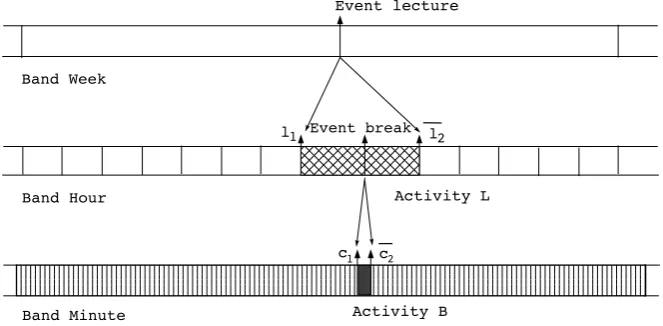
express its semantics. The newly explored process, the miracle, plays a crucial role in the construction of the timebands model to link all time bands as a whole. First, we use a lecture example to explain how to view a simple system in the timebands model. Suppose that one week a lecturer has a lecture which takes two hours and has a five-minute break. To model it, we define three time bands,Week,Hourand
Minute, which are given in an increasing finer order and illustrated in Fig.13.1. In BandWeek, eventlecturedoes not take any time to execute, but it is mapped into activityL with duration in BandHour. Furthermore, eventbreakin activity Lis mapped into another activityBin Bandminute. Thus, instead of mapping all events or activities into the finest band, we use some key events (or signature events) to link and integrate different bands into a whole. Meanwhile, the timebands model preserves consistency and coordination of the system in the multiple time scales. The timebands model is developed in a number of stages in this section including time bands, granularity and precision, simultaneous events and durative activities, and mappings between bands.
13.3.1 Time Bands
A system in the timebands model recognises a finite set of distinct time bands, and it always has the highest and the lowest bands that give a temporal system boundary. Each band is defined by a granularity, representing the basic unit of time in that band. This is different from temporal logic approaches which can represent a possibly infinite set of time bands.
The timebands model adopts discrete time, usually represented by non-negative integers. A granule is simply a set of time points and a granularity is a mapping
Gfrom integers to a granule. One healthiness condition [4] that granularity must satisfy is
Fig. 13.1 Mapping between different time bands
which states that any two granules of a granularity have no overlap and the elements of granules are ordered the same as their index order. A granuleG(i)can be com-prised of a single time unit, a set of contiguous units, or even a set of non-contiguous units. For example, the bank holidays for 2009 in England, defined as a collection of several days from different months, can be used as a granule.
Thus, the time bands in the lecture example can be defined as follows:
TBI= {Minute,Hour,Week}
Granularity(Hour,Minute)= {60}
Granularity(Week,Hour)= {7∗24}
The setTBI is a collection of the timeband identities. The functionGranularity de-fines conversion factors of different time bands’ granularities. These factors can be multiple. For example, a year may have 365 days or 366 days. In addition, the func-tionGranularityalso satisfies ‘finer than’ relations of different time bands. A granu-larityGisfiner thana granularityH if for each indexi, there exists an indexj such thatG(i)⊆H (j ). Conversion factors between two bands must be natural numbers, and therefore time bands are not always comparable. For example, a week band is not comparable to a month band.
13.3.2 Events and Precision
between events within a band such as instant events defined in Sect.13.2.9. Instan-taneity is the strongest constraint that is used especially to link different time bands via events and activities.
In specification of a system, events may cause an immediate response. For exam-ple, we consider such a requirement like ‘when the fridge door opens the light must come on immediately’. It actually means that the two events,door.openandlight.on, occur simultaneously but with an order. That is, the response is within the precision of the band. Precision, representing the measure of accuracy of events within that band, can only be expressed using the granularity of finer bands. Accordingly, two
simultaneousevents must, when viewed from a finer band, be within the precision of the current band. In respect to the finite number of time bands in the model, the finest (lowest) band has no precision. Due to precision, two simultaneous events cannot be exactly distinguished because the ‘gap’ between them is too small to be considered. Here the small gap also results in tolerance of the behaviours when mapping the two events into the corresponding activities of a finer band. For instance, considering the lecture example with three bands, precision can be defined as follows:
Precision(Week,Hour)=2
Precision(Hour,Minute)=5
If eventbreak is supposed to happen in the middle of a lecture, the precision of the hour band restricts the maximal duration of a break to be five minutes, other-wisebreakcannot be considered an instantaneous event in the hour band. Also, the precision allows the break to happen five minutes early or late.
Therefore, similar to the definition of instant events, the simultaneous operator is defined as follows:
P1
− →
#P2=P1;(P2◮ρ)
whereρ is the precision of that band. Two simultaneous events, e.g.,a andb, are expressed as eithera is beforeb or bis before a, but they must occur within the precision. We also use the following abbreviations to represent simultaneous events:
a−→#b=(a→SKIP)−→#(b→SKIP)
a#b=a−→#bb−→#a
where # denotes thata andb are simultaneous, and−→# that they are simultaneous but with an order. This abbreviation is applied to all simultaneous events in this chapter.
We cannot distinguish two simultaneous events in the current band; however, the interval between simultaneous events will be revealed in the form of precision when mapping these events to corresponding activities in a finer band. As a result, the precision basically plays two roles in a band: one is to measure accuracy of events such as simultaneous events, the other is to restrict the duration of activities. Un-fortunately, simultaneity is not transitive, i.e., the fact thataandbare simultaneous and so areb andc, does not imply that a andcare simultaneous. This also ele-gantly explains that a sequence of consecutively simultaneous pairs or repeatedly fast-moving events can be observing durative behaviours. We might not recognise any pair of them because the interval between them is less than the precision, but the whole duration may take a long time.
13.3.3 Punctual Clock-Tick Event
In modelling of real-time systems, we often employ ‘clocks’ to aid scheduling and coordination. We represent a default abstract clock in a band by defining each gran-ule as a ‘clock-tick’ event, which is modelled just like any other event. However these clock-tick events are forced to happen at same intervals by the deadline oper-ator. When necessary, more abstract clocks can be defined by the basic unit of time in the band. For example, the clock calledbusiness daysis placed in the day band; however, it is different from the default day clock.
Timed CSP is unlikely to explicitly represent clock-tick events because it can never guarantee that an event is able to happen precisely at a specific time point. The occurrence of events in timed CSP depends on their environment’s interaction even if the timeout operator is applied. However, this situation is entirely changed if we use the deadline operator. For example, we may simply define a punctual clock as follows:
C=((tick→SKIP)◮0);WAIT1;C
where the clock-tick eventtickmust occur precisely every time unit otherwise the punctual clock will not start.
We define clock-tick events for every time band, e.g., the clock-tick events for the lecture example given in previous section can be defined as follows:
Event:Minute mtick
Event:Hour htick
Event:Week wtick
An intuitive way to understand a clock-tick event is that it denotes a start point of a new time unit or the end point of the previous time unit. Therefore, for different clock-tick events in different time bands such asmtickandhtick, we say that the time interval between twohticksin the hour band contains 60mticks, rather than that an
events. That is to say, if a mapping is necessary, a clock-tick event in a higher band is mapped to an activity in a lower band which contains only one clock-tick event.
Punctual clock-tick events provide us with extensive convenience to express clock-related properties. For example, iftickis a clock-tick event representing 1:00,
tick‡adenotes thatamust happen precisely at 1:00 even if we observe it in a finer band;tick#a means thatamust occur at 1:00 too, butais allowed to happen early or late within the bound of the precision;tick→a→SKIP states thata occurs only if its environment provides the offer, anda occurs exactly at 1:00 only if its environment is friendly.
Note that clock-tick events are just ordinary events and they become meaningful only if we let them happen precisely at intervals of one time unit. Therefore, we attach a local timer to any processes during their life cycles. For example, a process with a timer is defined as follows:
PT =((P;e→SKIP)|[ {tick, e} ]|Timer△ {e}SKIP)\ {e}
Timer=tick→Timer′
Timer′=WAIT1 ‡(tick→SKIP);Timer′
where the evente (e /∈αP )is used to stop the timer by the interrupt operator when
P terminates, and one time unit inWAIT is a local time unit depending on which band the process is defined in. Notice that such a timer does not record the dura-tion of its whole life cycle, while it starts only if the first clock-tick event of the process starts. By comparison with a globally punctual clock in a band, local timers to processes are able to effectively avoid the deadlock caused by synchronisation of clock-tick events.3For the sake of convenience, we directly define a process as usual and subsequently its timer is attached automatically.
We usually use a clock-related process to express a very strong constraint that ‘something must occur at certain time points’. For example, a processtick→a→ tick→SKIP means that a must occur between two clock-tick events. Hence, a well-defined clock-related process is one in which all clock-tick events cannot be blocked. For example, a counterexample can be as follows:
P=tick→tick→(WAIT2;(tick→SKIP))
where obviously the third tick cannot occur such that the local timer blocks the occurrence of all clock-tick events.
3One of the approaches to model-check a timed CSP process is to translate it into an untimed CSP
13.3.4 Activities
An activity is a special process with clock-tick events. Activities are detailed expla-nations of events of higher bands, and hence, to maintain consistency of a system, ‘qualified’ activities must satisfy the following three requirements:
1. An activity must start and also finish with clock-tick events. 2. An activity must have one or more signature events.
3. Duration of an activity must be no longer than the precision of a higher band in which its corresponding event is placed.
Requirement 1 states that an activity should be well placed in the band. If the activity cannot start or finish with clock-tick events, it is supposed to be replaced in a finer time band. For example, an activity may be defined as follows:
A=tick#a1;tick#a2;tick#a3
which means that the events such asa1,a2anda3are simultaneous with clock-tick
events, and the duration of the activity is two time units. Note thata1may actually
occur before the eventtickintick#a1, but we consider that Astill starts with the
clock-tick event sincetick anda1 cannot be distinguished in this time band. The
duration ofAis counted from the occurrence of the firsttick, and not from the start of the activity. That is, the activity may initially wait in silence until the coming of an explicit clock-tick event, and its duration is actually determined by how many clock-tick events it involves.
As Requirement 2, each activity must have one or more signature events, which is not only the major observation of the activity, but also the linking to the corre-sponding event in a higher band. For example,a2is a signature event in the activity Aand an overhead line is used to make it different from other ordinary events. An activity can have more than one signature event, which must be linked to the same event of a coarser band and only one of which can happen during the life cycle of the activity. For example, making a drink by a vending machine may have two choices, tea or coffee, which can be described as follows:
Drink=(tick#hotwater;tick#milk;tick→tick#tea)
(tick#hotwater;tick#milk;tick#coffee)
The duration of an activity should be no longer than the precision of a higher band; otherwise it cannot be considered an event of the higher band. This imperative requirement will be fulfilled when the activity is mapped, since the precision for the activity is not yet decided until the link with the event in the higher band has been established. For example, there are two activities,AandB, in a day band, but
AandB are linked to two events in a month band and a year band respectively; consequently, their precisions might be different.
following three examples are not well-defined activities which violate Require-ments 1–3, respectively:
A1=a→tick→b→SKIP
A2=tick→a→tick→b→tick→SKIP
A3=tick→a→A3
Because an activity is a clock-related process, we can control when the activity will happen by fixing any event of the activity to happen at a specific time. That is, the events in the activity are uninterrupted events, as introduced in Sect.13.2.9. For example, if we impose the signature eventa2of the above activityAto happen
at 10:00,a1must then happen at 9:00 andAmust finish at 11:00. In fact,Astarts
from the beginning of the system; howevera1, very similar to the event of (13.1) in
Sect.13.2.8, can occur only if the other event must occur later.
13.3.5 Mapping Between Bands
In the components of the model considered so far, all behaviours have been confined to a single band. The essence of the timebands model is to describe the behaviour of each component of a system in a best suitable time band, and compose the multiple-band behaviours regarding the properties to be verified. To achieve this goal, events in one band may need to be mapped into activities in finer bands.
Activities become useful only when they are linked with events in higher time bands. Processes defined in different time bands have no intersection except for the linking of events and activities. Those links are the one and only channel to integrate all behaviours of the timebands model. The establishment of the links is achieved by means of imposing the events and the signature events of the activities to be instant events, so that they are constrained to occur together at all time.
The linked pair of an event and an activity can affect each other to decide when they will occur in their own bands. Recall the lecture example illustrated in Fig.13.1. ActivityBcan be given the following behaviour:
Event:Minutec1, c2
Activity:MinuteB=c1#mtick;mtick→mtick→mtick→mtick→c2#mtick
This activity actually means that students have to take a 5-minute break and any shorter or longer break is not allowed. If we insist that eventbreakin the hour band must occur in the middle of the lecture, e.g., around 10:00 (eventbreak and the clock-tick event are simultaneous), and then eventc1in activityBcan only happen
between 9:50 and 10:00, on account of the five-minute precision. That is to say, the signature eventc2 can happen only between 9:55 and 10:05. We can also set the
in the time when eventbreakmust occur in the hour band. For example, if we say thatc2occurs at 9:50, and thenbreakin the hour band must occur between 9:00 and
10:00.
To maintain consistency and coordination between different time bands, we sim-ply make events and the signature events of corresponding activities instant. For example, the mapping in the lecture example can be defined as the following pro-cesses:
Link1=lecture‡l2
Link2=break‡c2
And then these processes are synchronised with other processes in the system on all events of the alphabets ofLink1 andLink2.
Finally, we use the lecture example, illustrated in Fig.13.1, to demonstrate the integration of time bands. Granularity, precision and clock-tick events have been defined in previous sections. In the week band, we specify that a lecture must occur within a week:
Event:Week lecture
LECTURE=wtick→lecture→wtick→SKIP
And activityL, expressing a two-hour lecture with a break, is defined in the hour band as follows:
Event:Hourl1, l2,break
Activity:HourL=htick#l1;htick#break;htick#l2
Before events and activities are linked together, processes defined in different time bands have no interaction at all. Thus, the system before mapping is expressed by an interleaving process:
S=LECTURE|||L|||B
And then the integrated system is constructed by linking eventslectureandbreak
with activitiesLandBrespectively:
SYS=S|[ {lecture, l2} ]|Link1|[ {break, c2} ]|Link2
In practice, the assumption of maximal progress enables events to occur as soon as possible. For example, the processLECTURE in the week band specifies that
lecture may happen anytime within a week, but without a constraint from other processes or bands it always happens at the beginning of the week. With respect to Fig.13.1,4 if the lecture example starts, wtick, htick andl1 will initially start
4The clock-tick events are not directly given in this figure, whereas the reader can easily find out
together;lecture cannot happen immediately because it is coordinated with l2 or
the thirdhtickin the hour band; c1in the minute band cannot happen because it
depends onbreak or the second htick in the hour band. Subsequently, after one time unit of the hour band,breakhappens; however,c2has occurred five time units
(within the precision) of the minute band earlier, sincebreakand the secondhtick
are simultaneous. Consequently, another hour later,l2andlecturehappen together.
13.3.6 Discussion
The revolution of the timebands model is to use a mapping between instantaneous events and durative activities to integrate different behaviours described in different time scales into a whole system. The key idea of the mapping is to use instantaneity of the events and the signature events of the corresponding activities, and integrity (uninterrupted events) of the activities to locate right positions for mapped entities. The above two distinct properties are achieved through applying the unique process, the miracle.
The time system of the timebands model is a combination of implicit time and explicit clock-tick events. Here implicit time, similar to time in timed CSP, is a global clock whose granularity is the basic time unit of the finest time band. How-ever, processes themselves do not have read-access to the clock which is rather used in the semantic framework for the analysis and description of processes. A clock-tick event is an observation of a single precise time of the global clock and it can be accessed by any process. Because clock-tick events are punctual, we can specify clock-related events which must occur at specific time points.
Every clock-related process has a local timer (a clock with clock-tick events), which turns out to be able to interfere with the accuracy of its local clock. We do not require that the local clock of a process must be synchronised with the global clock. For example, we lethtick‡a to express thata must happen at the beginning of an hour such as 1:00, while we make the signature event (such as a′) of the
corresponding activity simultaneous withmtickin the minute band. Thus,a′must
happen at 1:00 because it is instant toa, butmtick#a′allows its local clock, relative
to the clock of the hour band, to quick or slow a little bit within the precision of the minute band. Of course, the local clock of a process can be easily synchronised with the global clock. This property is very useful in modelling the behaviour of a distributed system where components may have asynchronous clocks.
13.4 Case Study
The mine pump example was first proposed by Kramer et al. [20] and later used by Burns and Lister [6] as case study for developing dependable systems. The mine pump system is used to control a pump to pump out the water which is collected in a sump. The mine has two sensors to detect when water is above a high level or below a low level. A pump controller switches the pump on when the water level becomes high and off when it goes below the low level. The system also monitors the level of methane, since a pumping operation during a dangerous methane level will cause explosion. Reading from all sensors, the operations of the mine pump should satisfy the following safety requirements:
1. The pump can be used only when the methane level is safe.
2. The pump must be switched on within an interval since the water level has be-come high.
3. The pump must be switched off within an interval whenever the methane level becomes dangerous.
In a mine, water and methane come from the environment. We assume that the change of the water level is slow, and the methane level is stable in most of the time but can incidentally change very fast. Therefore, we use two time bands, a minute band and a second band, to describe the slow changing of the water level and the dramatic changing of the methane level respectively. For example, a delay of few seconds may have no influence on the change of the water level, while it could be crucial for switching the pump off when the methane level suddenly be-comes dangerous. Granularity and precision between the two bands are defined as follows:
TBI= {Minute,Second}
Granularity(Minute,Second)= {60}
Precision(Minute,Second)=5
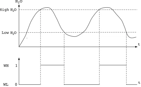
To simplify the modelling of the mine pump, we abstract the state of the water level as Fig.13.2by combining the values of two sensors for detecting the water level. That is, the state of the water level is low until water passes the high level, and it stays high until below the low level. This abstraction is reasonable since it is a practical decision to keep the pump on until the water level becomes low, though sometimes the pump has to be switched off due to the dangerous methane level.
Fig. 13.2 Sample timing diagram for water level
13.4.1 A Pump Controller
Depending on the states of the water and methane levels, a pump controller exe-cutes actions on the pump. Therefore, in the following implementation defined in the minute band, the system is basically decomposed into two components: one for monitoring the behaviour of water and the other for the behaviour of methane.
Event:Minute water.high,water.low,pump.on,pump.off,
methane.safe,methane.danger,mtick
WATERlow=water.high→(wl:=false;WATERhigh)
pump.off→WATERlow (13.3)
WATERhigh=water.low→(wl:=true;WATERlow)
pump.on→WATERhigh
¬ms&pump.off→WATERhigh (13.4)
METHANEsafe=methane.danger→METHANEdanger
pump.on→METHANEsafe
pump.off→METHANEsafe (13.5)
METHANEdanger=methane.safe→METHANEsafe
pump.off→METHANEdanger (13.6)
WATERlow in (13.3) states that the water level initially stays at the low level, and
it can become high through event water.high and still remain low if executing
pump.off. In addition,msandwlare two state variables to denote the safe methane and low water respectively. In the processWATERhigh, the eventpump.off can still
happen only if the methane level is dangerous.
These components must agree on when the pump is to be switched on or off. For example, before reaching the low water level during the pumping operation, the pump might be switched off due to the dangerous methane level. Afterwards, the pump has to be switched on again until the water level is below the low level.
CONTROL=WATERlow|[ {pump.on,pump.off} ]|METHANEsafe (13.7)
Without considering the timing issues, the above implementation CONTROL
clearly shows that eventpump.oncan occur only when the water level is high and the methane level is safe (becausepump.onis executed from processesWATERhigh
andMETHANEsafe). This satisfies the first safety requirement of the system.
How-ever, to make this system closer to reality, we will verify the other two more refined properties, which are going to be modelled in different time bands because of the different behaviours when the water and methane levels are changing.
13.4.2 Behaviour of Water and Methane in the Minute Band
Suppose that the change of the water level is slow and hence its behaviour is cap-tured in the minute band. The methane level is stable for most of the time, but can change very fast; e.g., it can reach the dangerous level in just few seconds. Obvi-ously, such a dramatic change of methane is best described in a finer time band such as the second band. In the following modelling, we will specify the different behaviours of the two components in the two time bands, depending on different scenarios.
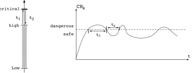
For modelling the change of the water and methane levels, we use worst-case execution time to describe the worst situations. As illustrated in Fig.13.3, the worst situation for water is that the water level has reached the high level but the pump cannot be switched on because the methane level just becomes dangerous. Hence, it is unnecessary to consider any operation when the water level is between the low and high levels if the worst case has satisfied the safety requirements. In practice, we always give a good safety margin to the value of the high level in case the pump cannot be switched on immediately. For example, the pump must be on withint1
time units after the water level becomes high, otherwise the mine fails. And the pump can take the water level below the high level if it has continuously worked fort2time units. If assuming thatr1andr2are the rates of change respectively at
Fig. 13.3 Assumptions on the change of water and methane
Thus, the time constraint of the behaviour of water and the related pump opera-tions in the minute band is modelled as follows:
TCW=water.high→HIGH(l1) (13.8)
HIGH(t1)=IFt1==0THEN(pump.on→ON(l1)
flooding→STOP)
ELSE(WAIT1;HIGH(t1−11)
pump.on→ON (l1−t1)) (13.9)
ON(t )=OFF(t∗r1/(r2−r1)) (13.10)
OFF(t2)=IFt2==0THEN pump.off→water.low→TCW
ELSE(WAIT1;OFF(t2−11)
pump.off→HIGH(l1−t2∗(r2−r1)/r1)
(13.11)
wheret, t1andt2 are time variables, andl1, r1andr2 are constants, e.g.,l1is the
maximal value of the bound oft1. The operator,IFbTHENP ELSEQ, is actually
a convenient shorthand of a guarded process,b&P¬b&Q.
The implementation in (13.9) states thatpump.onshould happen within some time units if the water level is high. The value oft1inHIGH(t1)is the deadline that
Accordingly, the timed behaviour of water and the pump is defined by the fol-lowing parallel composition:
A= {pump.on,pump.off,water.low,water.high}
TWATER=WATERlow|[A]|TCW (13.12)
The behaviour of methane in the minute band is relatively simple. Under the circumstance of worst-case execution time, we also assume two constants,l3andl4,
to be the maximal values of two time variables,t3andt4, as illustrated in Fig.13.3,
to denote the maximal duration of the dangerous methane level and the minimal duration of the safe level respectively.
TCM=methane.danger
→WAITl3;(methane.safe◮0);WAITl4;TCM (13.13)
TMETHANE=METHANEsafe|[ {methane.safe,methane.danger} ]|TCM (13.14)
And then, the system in the minute band can be finally modelled as follows:
TCONTROL=TWATER|[ {pump.on,pump.off} ]|TMETHANE (13.15)
Recall the safety properties which are introduced in the beginning of this sec-tion. Property 1 can be proved even under the untimed environment. The proof of Property 2 depends on the relationship among those constants. For example,l1is
obviously greater thanl3, otherwise the mine will fail since the pump cannot be
switched on in time. Ideally,l4is greater than l2orl1∗r1/(r2−r2)so that water
can be lowered below the high level once the pump is switched on. However, this requirement is too strict to accommodate many patterns of methane’s behaviour, e.g., the frequent oscillation around the dangerous level of methane does not satisfy this requirement. Therefore, it is more reasonable to satisfy a looser requirement thatl3/ l4is less thanl1/ l2within any interval (whose length should be greater than l1+l2).
13.4.3 Behaviour of Methane in the Second Band
First of all, we specify precision of the minute band to be 5 seconds, which directly determines the definition of simultaneity and the maximal duration of an activity. The delay of updating the state of water is ignored in the minute band, but it is considered in the second band. We assume the delay to be 2 seconds, and
water.high andwater.loware mapped into two activities, WHs andWLs, in the
second band respectively:
Activity:Second WHs=stick#high;stick→stick#whe (13.16)
Activity:Second WLs=stick#low;stick→stick#wle (13.17)
wherestick is a clock-tick event of the second band,wheandwledenote the end of the two activities respectively, andlow andhigh are two signature events. In addition, the activities are annotated for convenience.
Moreover, on account of the costing time on updating states and sampling fre-quency,methane.dangeris mapped into the following activity:
Activity:Second MDs=stick#danger;stick→stick→stick#mde (13.18)
And then, with regard to reaction delay,pump.offis mapped as well:
Activity:Second PFs=stick#command_off;stick
→stick#action_off (13.19)
where the eventaction_off denotes the genuine time when this command takes ef-fect.
Furthermore, we impose a constraint on all of these activities so that none of them can overlap each other because changing states presumably involves some computation:
ACTs=(WHs;ACTs)(WLs;ACTs)
(MDs;ACTs)(PFs;ACTs) (13.20)
To verify Property 3 in the second band, the activities in the above implemen-tation are integrated with the minute band by making their signature eventsinstant
with the corresponding events of the minute band. For the sake of simplicity,ACTs
is integrated withCONTROL, rather than TCONTROLwith time constraints, be-cause the ‘micro’ relation ofmethane.dangerandpump.off is irrelevant with those assumptions on how water and methane change.
CONTROLsecond=(CONTROL|||ACTs)
|[ {water.high,high} ]|Link3
|[ {water.low,low} ]|Link4
|[ {methane.danger,danger} ]|Link5
Note that these linking processes are just similar toLink1 andLink2 introduced in Sect.13.3.5. Even without the mechanised proof, intuitively, we recognise that Property 3 can be satisfied only if no other event in the minute band occurs between
methane.dangerandpump.off, since the total duration of the two events in the sec-ond band is 5 secsec-onds. That is, when executing the real program code, the program should directly implementpump.offwhen the methane level is dangerous instead of wasting time on updating the state of water.
13.4.4 Verification
To prove the three properties of the mine pump example by hand is error-prone since a number of obligations are discharged by obvious and intuitive assumptions where security breaches and system holes are usually hidden. However, establishing the mechanical proof in theorem provers is time-consuming, such as PVS [30] in which the semantics ofTCSPMhas been embedded and ProofPower [36] in which various
theories in UTP are mechanised. The model checker FDR [1] is very successful in efficiently verifying both safety and liveness properties of a system modelled in CSP. Therefore, timed CSP specifications can be implemented by FDR if they are translated into untimed ones. However, regardless of its expressiveness, the miracle cannot be expressed in FDR.
Timed automata [2,22] are powerful in designing real-time models with explicit clock variables, and a number of tools have been proved to be successful like the popular UPPAAL [21]. Timed automata are transition systems consisting of a set of states along with a set of edges to connect these states, and hence it is potential to express the miracle simply as an unstarted state. The idea of using timed automata to implementTCSPM or the timebands model is highly inspired by the work [11]
in which they define a set of composable timed automata patterns so that timed CSP can be translated to timed automata. Even if it is possible to represent the miracle in timed automata, the mechanism of the timebands model still involves a massive amount of work. For example, we need to develop a sound operational semantics of TCSPM which is usually described as a labelled transition system.
We also have to explore a trace-back technique for executing the model, since the fact that a process will not start if the deadline cannot be satisfied means that the process will go back to the unstarted state if the execution cannot go ahead. In the meantime, the observations which have happened during the execution will be erased, and the process just behaves like it has never started. All in all then, the work of fully analysing the timebands model in timed automata is in progress, and therefore the following verification of the mine pump example in UPPAAL simply provides a flavour to show how it will be possible to prove properties in a model checking approach.
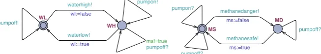
Fig. 13.4 The pump controller without time constraints
logic) [3]. More explanations of UPPAAL will be given along with the modelling of the mine pump example. First, the processCONTROLin (13.7) is modelled as two timed automata in Fig.13.4. Locations (or states) of a timed automaton are graphi-cally represented by circles where the overlapped circle is the initial location. Each location has an invariant which is an expression of conditions, and the program con-trol can stay on this location only if its invariant is satisfied. A transition is a jump from one location to another through an edge which usually consists of three parts: guard, synchronisation and update. For example, illustrated in the left automaton of Fig.13.4, starting from the locationWH(WATERhigh), eventpumpoffis
synchro-nised (or fired) with another one in the right automaton only if the methane level is dangerous. As a result, Property 1 holds if the following query is satisfied:
A[] METHANE.MS and WATER.WH imply ms==true
which means that for all reachable locations, being in the locationsMETHANE.MS
andWATER.WHimplies thatms==true. Sincepumponcan be fired only from the locationsMSandWH, the fact that the methane level is always safe guarantees Property 1.
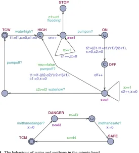
The behaviour of water and methane in the minute band,TCW andTCM, are represented by another two automata in Fig.13.5. Note thatxin both automata is a local clock that can be reset in the update part of an edge and used in a guard or an invariant. For example,xis reset during the transition from locationTCWto locationHIGH. Unfortunately, the value of a clock is not allowed to be assigned to any variable in UPPAAL, and that is why we define two integral variables,c1
andc2, to record how long the program control stays on the same location. UP-PAAL provides pair-wise synchronisation (one sender and one receiver) via regular channels and broadcast synchronisation (one sender and an arbitrary number of re-ceivers) via broadcast channels. However, a receiver in a broadcast channel can miss the synchronisation if it is not ready yet. Obviously, this is not same as the parallel in timed CSP orTCSPM. For example, in the mine pump example, the
synchronisa-tion onpump.onandpump.off involving three different processes cannot be directly expressed in UPPAAL. The solution is to use a shared variable (e.g.onandoff
Fig. 13.5 The behaviour of water and methane in the minute band
Fig. 13.6 The senders in a multicast synchronisation
In addition, urgent (labelled withU) and committed (labelled withC) locations are used in Fig.13.5. Time is not allowed to pass when the program is in any of the two locations, but an urgent location can engage in an interleaving. Notice that the approach to calculate the values oft1 andt2in Fig.13.5is different from the
one in (13.10) and (13.11) because a recursive process in the timebands model is measured by a descending order. To prove Property 2, we simply need to show the automata can never reach locationSTOPor eventfloodingcan not be fired if
l1> l3andl2< l4. Such a query can be expressed as follow:
A[] not TCW.STOP
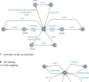
[image:28.439.199.387.381.439.2]Fig. 13.7 Activities in the second band
Fig. 13.8 The linking processes in the mapping
To verify Property 3, we should mechanise the miracle so as to express those pro-cesses and operators defined by the miracle. However, the embedding of the miracle in UPPAAL is still in progress. Here, regarding the mapping only in the mine pump example, we use an informal scheme to make sure coordination of events and activ-ities in different bands. For example, the processACTs, a collection of all activities
in the second band, in (13.20) is described as a timed automaton in Fig.13.7. The starting of each activity is guarded by a state variable which denotes whether the event in the minute band is ready to happen. For example, the bottom loop (corre-sponding toMDs) in Fig.13.7states thatdangercan happen only ifms==true,
and then the automaton waits three time units and finishes the activity with event
mde. The safe methane level means that the program control is staying on loca-tionMSas Fig.13.4, and hencemethanedangeris ready to occur. The linking processes likeLink3–Link6 are expressed as another automaton in Fig.13.8. The instantaneity of events and the signature events of activities is expressed by com-mitted locations which, however, cannot exactly describe this property because a committed location just means that time is not allowed to reside and an edge must be fired immediately. If the guard of the edge is not satisfied yet, the automaton is deadlocked.
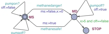
We add a new location with a guard in the automaton ofMETHANEsafein order
Fig. 13.9 The linking processes in the mapping
STOPmeans if the pump has not been switched off within five time units since the methane level becomes dangerous, the edge can lead to this location. Obviously, we need to prove the following query to be satisfied:
A[] not METHANE.STOP
The verifier of UPPAAL shows that the above query holds if we impose a constraint to exclude any other events betweenmethane.dangerandpump.off.
13.5 Conclusion
In this chapter we have formalised the timebands model using a new timed model (TCSPM) and shown how significantly the model contributes to describing dynamic
behaviours of complex real-time systems at many different time scales. Viewing a system as a collection of behaviours within a finite set of bands and integrating these behaviours through linking events and corresponding activities are a natural and effective approach to separate concerns and identify inconsistencies between different time bands of the system. We have also demonstrated the potential to use timed automata to implement the timebands model. Of course, it is still a long way to go for fully mechanising the timebands model. In future work we will apply the timebands framework to the analysis of more complex systems such as socio-technical systems. We believe that the modelling with a time-based hierarchy is able to help develop a comprehensive foundation to dependable systems.
Acknowledgements We would like to thank Ana Cavalcanti, Leo Freitas, Andrew Butterfield and Pawel Gancarski for discussions on the role of reactive miracles in programming logic, and thank Cliff Jones and Ian Hayes for discussion on the timebands model and possible approaches to formalisation. This work was partially supported by INDEED project funded by EPSRC:Grant EP/E001297/1.
References
1. Roscoe A.W.: Model-checking CSP. In: A Classical Mind: Essays in Honour of C.A.R. Hoare. Prentice Hall, New York (1994). Chap. 21
3. Alur, R., Courcoubetis, C., Dill, D.L.: Model-checking for real-time systems. In: LICS, pp. 414–425 (1990)
4. Bettini, C., Dyreson, C.E., Evans, W.S., Snodgrass, R.T., Wang, X.S.: A glossary of time granularity concepts. In: Temporal Databases, Dagstuhl, pp. 406–413 (1997)
5. Burns, A., Hayes, I.J.: A timeband framework for modelling real-time systems. Real-Time Syst.45(1–2), 106–142 (2010)
6. Burns, A., Lister, A.M.: A framework for building dependable systems. Comput. J.34(2), 173–181 (1991)
7. Ciapessoni, E., Corsetti, E., Montanari, A., San Pietro, P.: Embedding time granularity in a logical specification language for synchronous real-time systems. In: 6IWSSD: Selected Papers of the Sixth International Workshop on Software Specification and Design, pp. 141– 171. Elsevier, Amsterdam (1993)
8. Clifford, J., Rao, A.: A simple, general structure for temporal domains. In: Temporal Aspects in Information Systems, pp. 23–30. AFCET, Paris (1987)
9. Combi, C., Franceschet, M., Peron, A.: Representing and reasoning about temporal granular-ities. J. Log. Comput.14(1), 51–77 (2004)
10. Corsetti, E., Montanari, A., Ratto, E.: Time granularity in logical specifications. In: Proceed-ings of the 6th Italian Conference on Logic Programming, Pisa, Italy (1991)
11. Dong, J.S., Hao, P., Qin, S., Sun, J., Yi, W.: Timed automata patterns. IEEE Trans. Softw. Eng.
34, 844–859 (2008)
12. Franceschet, M., Montanari, A.: Temporalized logics and automata for time granularity. The-ory Pract. Log. Program.4(5–6), 621–658 (2004)
13. Group, T.R.L.: The RAISE Specification Language. Prentice Hall, Upper Saddle River (1993) 14. Hoare, C.A.R.: Communicating Sequential Processes. Prentice Hall International, Englewood
Cliffs (1985)
15. Hoare, C.A.R., Jifeng, H.: Unifying Theories of Programming. Prentice Hall International, Englewood Cliffs (1998)
16. Hobbs, J.: Granularity. In: Proceedings of the Ninth International Joint Conference on Artifi-cial Intelligence, Los Angeles, California, pp. 432–435 (1985)
17. Holzmann, G.: Spin Model Checker, the Primer and Reference Manual. Addison-Wesley, Reading (2003)
18. Holzmann, G.J.: The model checker SPIN. IEEE Trans. Softw. Eng.23(5), 279–295 (1997) 19. Jifeng, H.: From CSP to hybrid systems. In: A Classical Mind: Essays in Honour of C.A.R.
Hoare, pp. 171–189. Prentice Hall International, Hertfordshire (1994)
20. Kramer, J., Magee, J., Sloman, M., Lister, A.: CONIC: an integrated approach to distributed computer control systems. IEE Proc. E, Comput. Digit. Tech.130(1), 1–10 (1983)
21. Cardellini, V., Casalicchio, E., Grassi, V., Lo Presti, F., Mirandola, R.: Uppaal—a tool suite for automatic verification of real-time systems. In: Hybrid Systems III. LNCS, vol. 1066, pp. 232–243. Springer, Berlin (1995)
22. Lynch, N., Vaandrager, F.: Action transducers and timed automata. In: Formal Aspects of Computing, pp. 436–455. Springer, Berlin (1992)
23. Montanari, A., Ratto, E., Corsetti, E., Morzenti, A.: Embedding time granularity in logical specifications of real-time systems. In: Proceedings of the Third Euromicro Workshop on Real-Time Systems, Paris, France (1991)
24. Ouaknine, J., Schneider, S.: Timed CSP: a retrospective. Electron. Notes Theor. Comput. Sci.
162, 273–276 (2006)
25. Roscoe, A.W.: The Theory and Practice of Concurrency. Prentice Hall International, Engle-wood Cliffs (1998)
26. Sampaio, A., Woodcock, J., Cavalcanti, A.: Refinement inCircus. In: FME ’02, pp. 451–470. Springer, London (2002)
27. Schneider, S.: Timewise refinement for communicating processes. Sci. Comput. Program.28, 43–90 (1997)
29. Sherif, A., He, J.: Towards a time model forCircus. In: ICFEM ’02: Proceedings of the 4th International Conference on Formal Engineering Methods, pp. 613–624. Springer, London (2002)
30. Wei, K., Woodcock, J., Burns, A.: Embedding the timedCircusin PVS. Technical report. Available athttp://www-users.cs.york.ac.uk/~176kun/, University of York (2009)
31. Wei, K., Woodcock, J., Burns, A.: Formalising the timebands model in timedCircus. Technical report. Available athttp://www-users.cs.york.ac.uk/~kun/, University of York (2010) 32. Wei, K., Woodcock, J., Burns, A.: A timed model ofCircuswith the reactive design
mira-cle. In: 8th International Conference on Software Engineering and Formal Methods (SEFM), pp. 315–319, IEEE Comput. Soc., Pisa (2010).
33. Woodcock, J., Cavalcanti, A.: The semantics ofCircus. In: ZB ’02: Proceedings of the 2nd International Conference of B and Z Users on Formal Specification and Development in Z and B, pp. 184–203. Springer, London (2002)
34. Woodcock, J., Davies, J.: Using Z: Specification, Refinement, and Proof. Prentice Hall, Upper Saddle River (1996)
35. Yong, X., George, C.: An operational semantics for timed RAISE. In: FM ’99: Proceedings of the Wold Congress on Formal Methods in the Development of Computing Systems— Volume II, pp. 1008–1027. Springer, London (1999)