Reckoning Network Lifetime Ratio for Wireless Sensor Network

(1)

International Journal of Innovative Technology and Exploring Engineering (IJITEE) ISSN: 2278-3075, Volume-8 Issue-11, September 2019

Reckoning Network Lifetime Ratio for Wireless

Sensor Network

Mohamed Najmus Saqhib, Lakshmikanth .S

Abstract: Advanced Technologies such as Internet of Things, Machine Networking give rise to the deployment of autonomous Wireless Sensor Nodes. They are used for various domains namely battlefield monitoring, enemy detection and monitoring the environment change. These Wireless Sensor Nodes have the properties of low cost and high battery life. NL (Network Lifetime) is an important phase of Wireless Sensor Network (WSNs), in which the nodes can maintain sensing for a more amount of time. NL can be improved by use of multiple techniques namely Opportunistic Transmission, Scheduling of Timed Data Packets, Clustering of Nodes, Energy Harvesting and Connectivity. This paper provides the energy consumption computation, life time ratio definition and the overview of NL improvement techniques. The paper also presents brief review of the Destination based and Source based routing algorithm.

Keywords— Energy Harvesting, Lifetime Ratio, Wireless Sensor Network, Network Lifetime, Beam forming

I. INTRODUCTION

W

ireless Sensor Networks (WSNs) can be classified into cluster based network and single area random networks. Cluster based network will divide the entire area into a set of sub-areas. Each of the area will have a set of nodes. One among the node is chosen as the cluster head for communication between nodes of different clusters [1]. In order to have a better aerial communication a new application layer is provided which will have ContikiMAC layer along with IEEE 802.15.4 2.4 GHz physical layer. With this modification better efficiency energy, high reliability is obtained [2].

The information needed for placement of multiple target sources is provided by acquisition of Received-signal-strength (RSS) values with the help of inexpensive sensors.

Three algorithms are used to estimate the value of transmission power, location and orientation of target sources [3]. WSNs have higher advantage as compared to wired networks with respect to flexibility and easy access. Sequential Scanning is responsible for scanning of channels one by one, sensor nodes will be divided into subset and for each subset sequential scan is performed and the last approach will make use of randomized approach in which channel is assigned a random value [4].

Wireless Medical Sensor Networks (WMSNs) will be used for remote patient monitoring. The characteristics of environment are delay sensitivity and critical data. When the data is transmitted to the actual intended node at regular intervals at a higher rate causes issues like packet drops, retransmissions, and collisions [5].

Revised Manuscript Received on September 05, 2019

Mohamed Najmus Saqhib*, Research Scholar VTU Belgavi, Research Centre is Department of Electronics and Communication, Vivekananda

Institute of Technology, Bangalore, India. Email:

saqhibkhan89@gmail.com

Dr Lakshmikanth .S, Associate Professor, Department of Electronics and Communication Engineering, Acharya Institute of Technology, Bangalore, India. Email:lakshmikanth18@gmail.com

Exponential cat swarm optimization (ECSO) [6] combines two algorithms. The first algorithm is exponential weighted moving average and second algorithm is cat swarm optimization (CSO). In this algorithm cluster head is opted based on fuzzy-based ant colony optimization (PFuzzyACO) which computes fuzzy, ACO and penguin search optimization. The optimized routing algorithm finds an efficient route between the initiate and terminate node based on multiple parameters namely trust computation, energy value, delay value and density based computation of traffic. The taxonomy of applications in which WSN spans is summarized in Fig1.

Fig1: Application of WSNs

Fig 1 shows the applications in which WSN is used in a large amount namely Military, Health Care, Ocean Monitoring and Environment monitoring.

II. CLASSIFICATIONOFWSN

The broad classification of network is described in Fig2. There are two kinds of classification. The first kind is single area network and then second kind is cluster based network.

Fig2: Classification of Wireless Sensor Network

Single Area Network has all the nodes spread within an area at randomly locations and each of the node will communicate with other node in the network using its own specific algorithm and there is no controlling authority. The Single Area Network is

provided in the Fig3.

WSN Classification

Single Area Network Cluster Based Network

Military Application

Environment Monitoring Application of WSN

Ocean Monitoring Health Care

(2)

Fig3: Single Area Network

Fig3 shows the Single Area Network of size 100*100. As shown in the fig3 the nodes are spread randomly across the entire area. Node 9 is placed at (8, 10). Node 20 is placed at the location (1, 79). In a similar fashion, all the 100 nodes are placed at specific locations in the network.

The cluster-based network will spread the nodes across multiple clusters. Each cluster will have a specific set of nodes in the network. The communication between the nodes can happen directly if the initiator and terminator node is within the same cluster. Otherwise, the communication will happen through a special node of sufficient capacity known as the leader node. Cluster-Based Network is shown in Fig 4

0 10 20 30 40 50 60 70 80 90 100

1 2

3 4

5

6 7

8 9 10

11 12

13 14

15 16

17 18

19 20

21

22

23

24

25

26 27

28

29

30 31 32

33 34

35 36

37

38

X Position for Nodes

Y

P

o

s

it

io

n

f

o

r

N

o

d

e

s

Cluster Formation for Iteration

Fig4: Cluster -Based Network

Fig4 shows the cluster-based network. As shown in the Fig4 the nodes are spread across four different clusters. In the Cluster1 there are five nodes Node1 to Node 5 with the area of (1, 50) and (1, 50). Cluster2 contains 10 nodes within the area of (51,100) and (1, 50). Cluster 3 contains 8 nodes within the area of (1,50) and (51,100) and Cluster 4 contains 15 nodes within the area of (51,100) and (51,100). Section II will describe the energy loss process. Section III will define the lifetime ratio. Section IV will provide the definition of network lifetime in the literature. Section V will cover methods that can be used to improve the Network Lifetime.

III. ENERGYCONSUMPTION

The energy consumption [7]-[10] for the transmission of data is given by the equation



d

E

_c



2 *

_tx



_gen (1)

Where, Etx is the energy required for transmission, Egen is the energy consumed for packet generation, d is the distance between the nodes and then delta on top of the d is the attenuation factor.

The nodes in the coverage area are classified into Non- Healthy and Super Healthy nodes in the network. Healthy Nodes are set of nodes whose remaining energy will be less than four times the initial energy and Super Healthy nodes are the nodes whose remaining energy is higher than four times the initial energy or equal to it

Fig5: Classification of Nodes in the Coverage Area

[image:2.595.319.547.280.413.2]

Fig5 shows the Healthy and Super Healthy nodes. Consider that there are 10 nodes in the network and all the nodes are initialized with the same amount of energy of 500 J as provided in the Table1

Table- I: Initialize Energy of Nodes

Node Residual Energy

1 500

2 500

3 500

4 500

5 500

6 500

7 500

8 500

9 500

[image:2.595.302.551.519.656.2]

10 500

Table I shows the residual energy, as shown in the table all the nodes are initialized with same amount of energy of 500J.

The value IBE/4 = 500/4 = 125 J. Consider the routing path is 2 578

The routing path contains the route having Node2, Node4, Node 7 and Node 8.

Assuming the distance between the nodes as defined in the table II

Non-Healthy Super Healthy

<

4 IBE

_>=

4

(3)

[image:3.595.51.284.671.789.2]

Table- II: Distance between Nodes

Link Between Two Nodes Distance From Topology

2 5 20.24

5 7 45.56

7 8 34.56

Since Node-2, Node-5, Node-7 and Node-8 participate in routing they tend to lose their energy when they participate in routing

The Updated Energy is defined using the following equation

UEnode = CEnode – Ec (2)

Where,

CEnode = current energy of node

UEnode = update energy of node

E_c= Energy consumed

The updated energy of Node2 after the link is established between 25

UE2= CE2- Ec25 = 500- (2* 20+ 10* d25^0.5) = 500 –

(2*20+10*20.24^0.5) =415.0111 J

In a similar fashion the updating of Node 4 energy level and updating of Node 6 energy level

UE4= CE4- Ec46 = 1000- (2* 20+ 10* d46^0.5) = 500 –

(2*20+10*45.56^0.5) =392.5019 J

UE6= CE6- Ec68 = 1000- (2* 20+ 10* d68^0.5) = 500 – (2*20+10*34.56^0.5) =401.2122 J

The updating of energy levels after the routing path is established is given in Table III

Table- III: Updated Energy Levels

1 500

2 415.0111

3 500

4 392.5019

5 500

6 401.2122

7 500

8 500

9 500

10 500

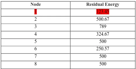
When the nodes participate in data delivery and routing over a period of time there residual energy keeps on decreasing. Consider after a period of 50 iterations the following is the energy level of the nodes in the network. As shown in Table5 Node1 and Node 9 are non-healthy Nodes and remaining nodes will be 2, 3, Node-4, Node-5, Node-6, Node-7, Node-8 and Node-10 will be Healthy nodes.

Table IV: Energy Levels after 50 iterations

1 123.45

2 500.67

3 789

4 324.67

5 500

6 250.57

7 500

8 500

9 110.87

10 500

IV. LIFETIMERATIO

The Lifetime Ration is a measure that helps in maintaining a healthy network with a sufficient amount of capacity to transfer the critical data packets in the network. The Lifetime ratio is used as an important parameter in determining the performance of an algorithm. The lifetime ration is defined as below

4 /

IBE

RE

with

nodes

of

count

IBE

RE

with

nodes

of

count

LR







(3)

When the nodes participate in data delivery and routing over a period of time there residual energy keeps on decreasing and hence as the iteration increases the lifetime ratio also comes down.

Fig6: Residual Energy Dependency of a Specific Node

Fig6 shows the Residual Energy of Node. As shown in the fig if the initial energy of the node is 3000 J as the number of times the node participates in routing the residual energy keeps on coming down.

(4)

[image:4.595.51.287.66.268.2]

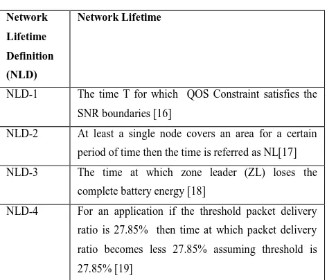
Table V: Network Lifetime Definition

Network

Lifetime

Definition

(NLD)

Network Lifetime

NLD-1 The time T for which QOS Constraint satisfies the

SNR boundaries [16]

NLD-2 At least a single node covers an area for a certain

period of time then the time is referred as NL[17]

NLD-3 The time at which zone leader (ZL) loses the

complete battery energy [18]

NLD-4 For an application if the threshold packet delivery

ratio is 27.85% then time at which packet delivery

ratio becomes less 27.85% assuming threshold is

27.85% [19]

VI. NETWORKLIFETIMEENHANCEMENT

TECHNIQUES

There are lot of Network Lifetime Improvement techniques which are present in the literature but few of them can be categorized as given in the Fig 8

Fig7: Network Lifetime Enhancement Technique

Fig7 provides a few techniques that can be used in order to increase the lifetime of the network. Network Lifetime can be improved by making use of various techniques Opportunistic transmission and time scheduling, Energy Harvesting, Beamforming, Coverage and Connectivity constraint, Routing and Clustering techniques, Data Gathering and Resource Allocation

A. Energy Harvesting

Energy Harvesting is a promising technique in order to achieve a better lifetime ratio. Low Overhead based Energy Harvesting prediction method is provided by making use of multiple prediction models and helps in achieving a higher

amount of accuracy. The method achieves 26.4% reduction in battery capacity for efficient data transmission [20]. For an independent quarry application [21], self-driving trucks are responsible for collecting the goods from one point and then transport them to another point. WSNs are used in such an application in order to determine locations where goods must be picked up and provide reliable operating principles for quarry. Vehicle sends energy to WSN nodes which are within the coverage area and then the sensor makes use of the energy in order to send the data to vehicles and vehicles send this information to the Access Point. The Access Point acts as a unit that executes method/algorithms in order to improve the channel selection process and also achieve lesser interference. This will result in obtaining better energy utilization.

Multipurpose EnerGy-efficient Adaptable low-cost sensor Node (MEGAN) [22] provide techniques like flexibility, energy efficiency, reconfiguration of data in an Internet of Things (IoT) environment. The techniques make use of 32 kinds of sensors and actuators. Power management circuit is used at sensor nodes to improve the lifetime ratio of the network and also it makes use of unregulated energy resource so that it can recharge from energy resource at any point of time. Self-Sustainable energy [23] is obtained with the help of energy harvesting devices present at the node level. Collecting data from nodes in the network along with Minimum Latency Aggregation Scheduling (MLAS) is a problem statement that must be solved by providing the collection mechanisms with no cracks and reduce the time required for recharging the node. The cracks in the system are independent of time and the recharging process of the node depends on the change in the time. The better approach of collecting data would be obtaining the data from the subset of nodes which provides the sufficient amount of quality coverage and perform scheduling in an adaptive fashion depending on the residual energy of nodes in the network.

B. Routing and Clustering Techniques

Many applications of IoT make use of WSN Network and the expectation is to have the application with higher NL [24]. This makes it a priority to control overall energy consumption mechanics in sensor nodes by using extra energy generator for the node. EH-HL is a model that can be used to build smart homes by making use of energy harvesting and hybrid LiFi communication techniques. WSN can make use of either direct hop mechanism or multi-hop mechanism [25] in order to collect the data from a specific region and transmit it to Base Station (BS). Energy consumption limits the lifetime of the network and hence the design of the communication mechanism between the sensor nodes and Base Station is important. For each application i.e time-critical applications, periodic data transfer applications make use of specific protocols to improve lifetime.

LEACH is a hierarchically based routing protocol that divides the area into multiple subunits. Each subunit has a chosen leader node that is elected in a random probabilistic fashion. When the data packets are to be sent towards the sink node there is a lot of back and forth propagation that happens between the base station and the nodes in the network which directly

increases the energy

consumption and hence reduces the lifetime ratio in

Data Gathering

Resource Allocation

Coverage and Connectivity

constraint

Opportunistic transmission

and time scheduling

Beam Forming Energy Harvesting

Network Lifetime Enhancement

Technique Routing and

(5)

the network, In order to improve the network lifetime LEACH can be modified by making use of Cluster Chain Mobile Agent (CCMA) [26] mechanism which will allow the mobile agent to visit each subunit and do a data aggregation.

Clustering techniques help in reducing overall energy dissipation and improve the energy efficiency in the network. MZ-SEP protocol [27] divides the clusters into multiple zones of triangular shape and helps in reducing the overhead of communication between leader node and member nodes. MZ-SEP algorithm provides a longer stability period as compared to the SEP protocol. In order to provide the lifetime ratio improvement for the case of LEACH protocol the probability of selection is performed based on energy factor and is done on a sliding window [28].

when the nodes are used in an environment like fire detection, enemy vehicle tracking without making a subset then it leads to huge processing power, peak battery usage and useless redundant bits [29]. This can be reduced by dividing the area into subsets and making a subset based communication so that the overall NL is increased. Yet Another LEACH [30] protocol will improve the NL by making use of alternative leader nodes in each round and also if the leader node energy becomes below the threshold then another node vice leader node will act as a leader node, Energy dissipation is one of the most important constraints which is responsible for the reduction in NL [31]. When the clustering and routing are married in a right way then energy efficiency can be improved. In order save the power, the network coding is used during data transmission by the cluster head nodes which improves NL.

C. Beam Forming

It is a mechanism of using the sensor nodes in the right fashion to deliver the data to the right resource and send the jamming signal towards the wrong resource.

The generation of maximum radiation towards the actual user and side lobe towards the interference user is called Beam forming [32]-[38]. There are many techniques which are used to achieve beam forming like autocorrelation and cross-correlation computation using Sample Matrix Inverse, reducing the mean square error by making use of Least Mean Square

The antenna arrays which are distributed in nature will send selective beams towards the receiver which will increase the transmission range the amount of transmission power can be decreased by nodes due to energy dissipation being shared among the transmitting devices. By making use of collaboration in beam forming there can be a reduction in a load of traffic and data can be replicated even during critical battery charge status [39]

Energy-aware beam forming techniques have better performance as compared to normal beam forming techniques. The minimum sample rate at each node will be maximized because the energy consumption at the node level is smaller than the energy received by the node [50]. The electromagnetic waves can be used to supply the power to the sensor node. Directional wireless power transfer can be adjusted in an adaptive by making use of energy beam forming beacons (BFB) which can maximize the average received power [40].

D. Coverage and Connectivity constraint

The task distribution among the different nodes in the network is done for agriculture applications and for such applications reliable coverage becomes very important. The NL can be improved by providing reliable coverage [41]. The load balancer is used for providing reliable coverage in the field under sensor area and also provides good time connectivity with respect to the base station using NL maximum approach [42]

The active sensors can be used to provide full-time coverage for a specific region for a given duration; multi-hop communication is used to send the detected data towards the destination node [43]. The deactivate mode of the scheduler can be used to make the nodes switch between ON and OFF state in order to monitor the target regions [44] so that NL can be maximized.

The deep analysis of hierarchical logic mapping is done in order to solve the problem of sensing coverage. The classification of terrain based on attributes namely number of nodes and transmission data is done to maximize the NL [45]

E. Data Gathering

The entire route trace consists of multiple nodes. If one or multiple of such nodes fail then there are errors and the data will be lost. The burst errors can be corrected with the help of Low Rank Parity Check Code (LRPC) and also provides an efficient decoding rate. [46]

The data transfer is done towards the base station by the group of sensors in WSN. When there is huge data flow it reduces the NL. Small memory, limited energy and computation complexity along with other constraints limit the functionality of WSN [47]. In order to increase NL the zone based and tree-based method provides a decrease in EC.

The energy efficiency and NL improvement are done using E-PEGASIS [48] which is built on top of the PEGASIS protocol and the monitoring can be done in a proactive manner on hierarchical data routing protocols in order to improve energy levels and NL improvement.

F. Transmission and Time Scheduling

When the attenuation of the signal occurs with respect to time [11], geographical position and frequency then it is referred to as fading. The information is gathered by nodes, send them towards the control station, during the process of broadcasting the nodes which come in the routing trace will receive information. The lifetime of the network can be optimized by making the relay nodes to be in the sleep mode. Channel State data and remaining energy are attributes that help for improving NL.

The nodes which participate in the transmission process will be adjusting the power based on the remaining energy and CSI [45]. Monitoring of channel quality parameters and allowing the transmission only if channel quality exceeds thresholds will help in improving NL [49]. In an application where packet arrival rate is always constant in nature or arrival happens at fixed intervals then nodes can be made to sleep when packet arrival is not expected and then it will be awake when packets arrive [50].

The sleep scheduling with a reduction in energy dissipation [51] and join the routing

(6)

to a Fixed Process of scheduling.

The working of sensor networks is a controlled mechanism by making use of the duty cycle, neighbor discovery periods and data delivery rate. reduced-complexity Genetic Algorithm (GA) [52] can be used in Multi-hop networks with two kinds of scheduling algorithms which can be either random or it can be circular. The goal of the scheduler is to group a set of nodes into a cluster and select better clusters heads in an adaptive fashion with the help of genetic.

WSN is used by many civil organizations in order to monitor the physical activity of end-users and used in domains like health, agriculture, habitat monitoring, routing of traffic, military and security applications [53]. The sensed data is transmitted by sensors to gateways and then towards the controlling station in a multi-hop fashion, thus leading to energy consumption and reduction in lifetime ratio. The energy-aware framework makes use of the duty cycle schedule to configure the nodes in an efficient way to reduce node and network-level energy consumption. G. Resource Allocation

The resources are needed for a wide variety of use cases like routing, scheduling, placement of nodes, throughput maximization, and adaptation of rate. The energy-efficient routes can be obtained on a dynamic topology by making use of sensors which can be switched between active and inactive mode on a MAC layer [54]. When the analysis of Link, Routing and MAC layer are performed then it will have multiple constraints like power allocation, link scheduling and energy dissipation which can be optimized using the cross-layer approach in order to minimize the ED which in turn can improve the NL [55]. For a water quality detection in rivers, WSN nodes are used is anomaly detection which requires more power which can be reduced by switching nodes between active and idle modes at the regular time [56].

UAV-mounted base stations (UBS's) [57] are used to provide services over a wireless network with few resources. User-based association and resource allocation are used to perform the optimization of multiple USBs cables. The optimization of the network is performed by making use of effective spectrum and resource allocation. Multi-Hop communication makes use of distributed agents which are of low cost and also offer a high amount of flexibility [58]. Since there are many distributed agents then for communication the agents have to make use of a resource that is shared. The energy savings can be done with the help of an event and a self-triggered system in which the amount of transmission to be done is informed before transmission actually occurs and resources are provided by the system.

Distributed resource allocation [59] has an inefficiency when agents compete to reduce the cost constraint by total resource and capacity. Ermeng Fu and the team describe a cost function that can get good objective function with limited conditions.

Heterogeneous networks are a combination of macro and femtocells and improve the capability of the network. When the environment is changed to a mobile then there will be frequent handover and abrupt resource allocation. Mobility prediction scheme [60] makes use of the Hidden Markov Model (HMM) which predicts the location of UE and thereby allocates the set of resources.

VII. NETWORKPROTOCOL

This section describes various protocols responsible for sending data packets between source nodes to destination node on the basis of path establishment.

A. DSDV Algorithm

DSDV(Destination Sequence Distance Vector), [61] makes use of table driven techniques with node level routing information maintenance for all the destinations. The updating of routing information is done at regular intervals. DSDV will find the set of initiators with dual coverage range. From each of the initiators to the destination the route is found out from the source node to destination node based on rules. The route discovery time is found out for all the discovered routes and then finally the route which has the lowest route discovery time is chosen as the best route.

The algorithm will find the neighbor nodes. If the neighbor nodes have the destination node then routing process is stopped otherwise the nodes in the forward direction are picked up in the coverage area and after that the forward node is picked up based on rules. Like this process is repeated till the sink is reached.

Suppose there are Nr routes which have been found then the route which has the lowest route discovery time will act like a best route.

time

route

i

t

Where

t

T

th i

Nr DSDV



,

}

.

...

,...

,

min{

₁ ₂

(4)

B. AODV Algorithm

In AODV (Ad-Hoc on Distance Vector) there is no route which is maintained from each node in the network. A set of unique nodes known as precursor nodes is responsible for performing route maintenance and route is found out only during it is required. AODV is developed on top of DSDV and is used find the multiple routes with initiator within the transmission range. The distance is found from each of the routes and then best route is the one which has the lowest distance.

distance

route

i

d

,

}

.

...

,...

,

min{

th i

2 1



Where

d

BRC

_AODV _Nr

(5)

C. ZRP Algorithm

ZRP (Zone Routing Protocol) routing will find the neighbors. After that the neighbors are segregated into border nodes. From each of the border nodes the individual route discovery is performed. After that the route which has the lowest time is chosen as the best route. The individual route discovery is performed by making use of use of the following process

While performing individual route discovery using ZRP. The distance with respect to each of the zone nodes is found out. The nodes which are within the transmission range are found out. If the nodes have the destination node then stop the routing process. If the nodes does not have destination node then round trip time is computed from each of the coverage zone nodes. After that the node which has the lowest time is chosen as the

(7)

D. EEDR Algorithm

The EEDR (Energy Efficient Destination Routing algorithm) makes use of receiver node in order to perform the CRN packets broadcasting. The forward node will be picked from the cover set nodes by measuring the channel quality and the node which has highest channel quality will be treated as the next forwarding node.

The sequence of execution will involve multi valued steps with first step being the path discovery, the second one is the forwarding mechanism for packet, and the selection of routing values and finally process necessary in data sending is involved. First the initiator will send the CRN packets to the cover set nodes. The received CRN packet SNIR values are used to compute the CQI values. The forward node will pick the highest CQI value. The process is repeated until path is established.

For individual route discovery in EEDR routing process, the distance is computed with respect to other nodes in the network, once the neighbor nodes are found out then a check is performed whether neighbor nodes have the destination node. If the destination node is present this stop the routing process. If the destination node is not present in the transmission range then CQI is computed for all the neighbor nodes and the node which has the highest value of CQI will be chosen as the next forwarding node. Each time a hop is established threshold count will be reduced. Once the threshold count is zero then Min Hop based path is established. The following are the summarized view of literature implemented algorithms

Table VI: Comparison of different routing algorithms

Algorithm Advantages Disadvantages

DSDV _{Best Route is found out}

based on lowest route discovery time

Too many routes are found out which increases the complexity of routing algorithms

Back and Forth propagation occurs during the route path analysis

Forward Node Pick is based on static rules

AODV The amount of routes

that are found are less than AODV

The route which has the lowest distance in the end to end routing path is found out.

Forward Node is picked based on static rule

Energy consumed is very high.

Number of Dead Nodes are very high

Lifetime ratio is very less

ZRP As compared to AODV

ZRP does not have an overhead of route

maintenance and

dynamic route is found out based on zones

Delay is less than DSDV and AODV

Forward Node is picked based on REPLY time and

does not take into

consideration channel quality

Number of Dead Nodes is more

Throughput is lesser

EEDR EEDR algorithm will

find the route based on receiver value point

EEDR will pick the best route based on highest value of CQI

The forward node will be find based on good amount of SNR

EEDR picks the forward purely based on CQI and

does not take into

consideration the residual energy of the node

EEDR has high amount of routing overhead

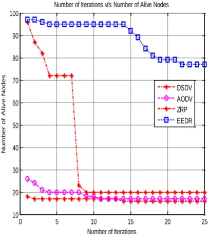
VIII. SIMULATIONRESULTS

[image:7.595.310.552.48.153.2]

This section will describe the simulation of network lifetime for the algorithms – DSDV, AODV, ZRP and EEDR.The simulation input is summarized by making use of following table

Table VII: Simulation Input Parameter

Name

Parameter Value

Number of Nodes 100

Area 100*100

Transmission Range 40m

Energy Required for Transmission

20 mJ

Energy Required for Generation

10 mJ

Attenuation Factor 0.5

Initial Energy 1000 mJ

Threshold Count 4

A. Lifetime Ratio Computation

If IB is the initial battery energy then count of set of nodes whose remaining energy are higher than or equal to IB/4 will provide information about number of alive nodes.

0 5 10 15 20 25

10 20 30 40 50 60 70 80 90 100

Number of Iterations

N

u

m

b

e

r

o

f

A

li

v

e

N

o

d

e

s

Number of Iterations v/s Number of Alive Nodes

DSDV AODV ZRP EEDR

Fig 8: Number of Alive Nodes

[image:7.595.320.531.229.383.2] [image:7.595.322.525.436.674.2]

(8)

0 5 10 15 20 25 0

10 20 30 40 50 60 70 80 90

N

u

m

b

e

r

o

f

D

e

a

d

N

o

d

e

s

Number of Iterations v/s Number of Dead Nodes

[image:8.595.63.258.56.308.2]

DSDV AODV ZRP EEDR

Fig 9: Number of Dead Nodes

The count of set of nodes whose remaining energy is less than IB/4 is called as dead nodes. Fig 9 shows the number of dead nodes in the network. As shown in the fig EEDR has the lowest number of dead nodes followed by ZRP, AODV and DSDV. EEDR is performing the best with respect to number of dead nodes.

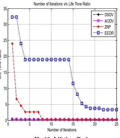
0 5 10 15 20 25

0 5 10 15 20 25 30 35

L

if

e

Ti

m

e

R

a

ti

o

Number of Iterations v/s Life Time Ratio

DSDV AODV ZRP EEDR

Fig 10: Lifetime Ratio

The lifetime ratio is defined as the ratio of number of alive nodes to the number of dead nodes. As the iteration increases the lifetime ratio will decrease. EEDR has the highest lifetime ratio followed by ZRP, AODV and DSDV.

IX. CONCLUSION

Prolonging the life of network in wireless networks has become a major field of research; it is also a complex task as multiple parameters wield influence on battery consumption in WSN. In this paper discussion is made about applications of WSN network. The Classification of network is done into two kinds namely Single Area

Network and Cluster based network. Energy Loss Computation is described along with Lifetime ratio. Various existing definitions of network lifetime has been reviewed. The various techniques that are used for improvement of lifetime namely Energy Harvesting, Beam forming, Routing and clustering techniques, Opportunistic routing and Time Scheduling and Data Gathering are briefly described. The algorithms namely DSDV, AODV, ZRP and EEDR are also described in this paper. It can be observed from the simulation result that as the iteration increases the lifetime ratio will decrease. EEDR has the highest lifetime ratio followed by ZRP, AODV and DSDV.

REFERENCES

1. Murugaanandam.S. and Ganapathy.V., "Reliability-based Cluster Head Selection Methodology using Fuzzy Logic for Performance Improvement in WSNs," in IEEE Access.

2. Y. Qin, D. Boyle and E. Yeatman, "Efficient and Reliable Aerial Communication with Wireless Sensors," in IEEE Internet of Things Journal.

3. P. Zuo, T. Peng, K. You, W. Guo and W. Wang, "RSS-based Localization of Multiple Directional Sources with Unknown Transmit Powers and Orientations," in IEEE Access.

4. L. Spyrou, P. Chambers, M. Sellathurai and J. Thompson, "Tradeoffs in Detection and Localisation Performance for Mobile Sensor Scanning Strategies," 2019 Sensor Signal Processing for Defence Conference (SSPD), Brighton, United Kingdom, 2019, pp. 1-5. 5. A. R. Bhangwar et al., "WETRP: Weight based Energy &

Temperature aware Routing Protocol for Wireless Body Sensor Networks," in IEEE Access.

6. P. K. H. Kulkarni and P. Malathi Jesudason, "Multipath data transmission in WSN using exponential cat swarm and fuzzy optimisation," in IET Communications, vol. 13, no. 11, pp. 1685-1695, 16 7 2019.

7. V. Potdar, A. Sharif, and E. Chang, "Wireless sensor networks: A survey," in Advanced Information Networking and Applications Workshops, International Conference on 2009, pp. 636-641. 8. V. Gungor and G. Hancke, “Industrial wireless sensor networks:

Challenges, design principles, and technical approaches,” IEEE Transactions on Industrial Electronics, vol. 56, no. 10, pp. 4258– 4265,October 2009.

9. “Wireless sensor networks: A survey,” Computer Networks,vol. 38, no. 4, pp. 393–422, March 2002.

10. K. Romer and F. Mattern, “The design space of wireless sensor networks,” IEEE Wireless Communications, vol. 11, no. 6, pp. 54– 61,December 2004.

11. Dietrich and F. Dressler, “On the lifetime of wireless sensor networks,”ACM Transactions on Sensor Networks, vol. 5, no. 1, pp. 1–39,February 2009.

12. M. Najimi, A. Ebrahimzadeh, S. Andargoli, and A. Fallahi, “Lifetime maximization in cognitive sensor networks based on the node selection,” IEEE Sensors Journal, vol. 14, no. 7, pp. 2376–2383, July 2014.

13. Y. Chen and Q. Zhao, “On the lifetime of wireless sensor networks,” IEEE Communications Letters, vol. 9, no. 11, pp. 976–978, November 2005.

14. J. W. Jung and M. Weitnauer, “On using cooperative routing for lifetime optimization of multi-hop wireless sensor networks: Analysis and guidelines,” IEEE Transactions on Communications, vol. 61, no. 8,pp. 3413–3423, August 2013

15. C. Cassandras, T. Wang, and S. Pourazarm, “Optimal routing and energy allocation for lifetime maximization of wireless sensor networks with nonideal batteries,” IEEE Transactions on Control of Network Systems, vol. 1, no. 1, pp. 86–98, March 2014.

16. B. Bejar Haro, S. Zazo, and D. Palomar, “Energy efficient collaborative beamforming in wireless sensor networks,” IEEE Transactions on Signal Processing, vol. 62, no. 2, pp. 496–510, January 2014

17. M. Bhardwaj and A. P. Chandrakasan, “Bounding the lifetime of sensor networks via optimal role assignments,” in IEEE International Conference on Computer Communications (INFOCOM’02), vol. 3, NY,USA, June 2002, pp. 1587–1596.

[image:8.595.64.263.408.637.2]

(9)

Distributed Processing Symposium, Denver, CO, April 2005 19. B. C˘arbunar, A. Grama, J. Vitek, and O. C˘arbunar, “Redundancy

and coverage detection in sensor networks,” ACM Transactions on Sensor Networks (TOSN), vol. 2, no. 1, pp. 94–128, February 2006. 20. X. Li and N. Xie, "Multi-Model Fusion Harvested Energy Prediction

Method for Energy Harvesting WSN Node," 2018 IEEE International Conference on Electron Devices and Solid State Circuits (EDSSC), Shenzhen, 2018, pp. 1-2.

21. V. N. Vo, H. Tran, E. Uhlemann, Q. X. Truong, C. So-In and A. Balador, "Reliable Communication Performance for Energy Harvesting Wireless Sensor Networks," 2019 IEEE 89th Vehicular Technology Conference (VTC2019-Spring), Kuala Lumpur, Malaysia, 2019, pp. 1-6.

22. S. Misra, S. K. Roy, A. Roy, M. S. Obaidat and A. Jha, "MEGAN: Multipurpose Energy-Efficient, Adaptable, and Low-Cost Wireless Sensor Node for the Internet of Things," in IEEE Systems Journal. 23. K. Chen, H. Gao, Z. Cai, Q. Chen and J. Li, "Distributed

Energy-Adaptive Aggregation Scheduling with Coverage Guarantee For Battery-Free Wireless Sensor Networks," IEEE INFOCOM 2019 - IEEE Conference on Computer Communications, Paris, France, 2019, pp. 1018-1026.

24. P. K. Sharma, Y. Jeong and J. H. Park, "EH-HL: Effective Communication Model by Integrated EH-WSN and Hybrid LiFi/WiFi for IoT," in IEEE Internet of Things Journal, vol. 5, no. 3, pp. 1719-1726, June 2018.

25. K. K. Pandey, B. Saud, B. Kumari and S. Biswas, "An energy efficient hierarchical clustering technique for wireless sensor network,"2016FourthInternational Conference on Parallel, Distributed and Grid Computing (PDGC), Waknaghat, 2016, pp. 544-549.

26. S. Sasirekha and S. Swamynathan, "Cluster-chain mobile agent routing algorithm for efficient data aggregation in wireless sensor network," in Journal of Communications and Networks, vol. 19, no. 4, pp. 392-401, August 2017.

27. A. Mahboub, E. M. En-Naimi, M. Arioua, I. Ez-Zazi and A. El Oualkadi, "Multi-zonal approach clustering based on stable election protocol in heterogeneous wireless sensor networks," 2016 4th IEEE International Colloquium on Information Science and Technology (CiSt), Tangier, 2016, pp. 912-917.

28. S. Poolsanguan, C. So-In, K. Rujirakul and K. Udompongsuk, "An enhanced cluster head selection criterion of LEACH in wireless sensor networks," 2016 13th International Joint Conference on Computer Science and Software Engineering (JCSSE), Khon Kaen, 2016, pp. 1-7.

29. N. Kumar and S. Kaur, "Performance evaluation of Distance based Angular Clustering Algorithm (DACA) using data aggregation for heterogeneous WSN," 2016 International Conference on Computation of Power, Energy Information and Commuincation (ICCPEIC), Chennai, 2016, pp. 097-101.

30. W. T. Gwavava and O. B. V. Ramanaiah, "YA-LEACH: Yet another LEACH for wireless sensor networks," 2015 International Conference on Information Processing (ICIP), Pune, 2015, pp. 96-101.

31. H. Y. Shwe and P. H. J. Chong, "Cluster-Based WSN Routing Protocol for Smart Buildings," 2015 IEEE 81st Vehicular Technology Conference (VTC Spring), Glasgow, 2015, pp. 1-5. 32. Faezeh Alavi, Kanapathippillai Cumanan, Zhiguo Ding, Alister G.

Burr,"Beamforming Techniques for Non-Orthogonal Multiple Access in 5G Cellular Networks", IEEE Transactions on Vehicular Technology, 2018

33. Irfan Ahmed, Hedi Khammari, Adnan Shahid, Ahmed Musa, Kwang Soon Kim, Eli De Poorter, Ingrid Moerman,"A Survey on Hybrid Beamforming Techniques in 5G: Architecture and System Model Perspectives",IEEE Communications Surveys & Tutorials,2018 34. Devashish Arora, Meenakshi Rawat, "Comparative analysis of

beamforming techniques for wideband signals", International Conference on Computing and Communication Technologies for Smart Nation (IC3TSN),2017 Pages: 51 – 54

35. Pogula Rakesh, S. Siva Priyanka,T. Kishore Kumar, "Performance evaluation of beamforming techniques for speech enhancement",Fourth International Conference on Signal Processing, Communication and Networking (ICSCN), Year: 2017, Pages: 1 – 5 36. Spyridon Vassilaras,George C. Alexandropoulos,"Cooperative

beamforming techniques for energy efficient IoT wireless communication", IEEE International Conference on Communications (ICC),Year: 2017,Pages: 1 – 6

37. Adnan Anwar Awan, Irfanullah, Shahid Khattak, Aqdas Naveed Malik, "Performance comparisons of fixed and adaptive beamforming techniques for 4G smart antennas", International

Conference on Communication, Computing and Digital Systems (C-CODE),Year: 2017 Pages: 17 – 20

38. Anupama Senapati, Kaustabh Ghatak, Jibendu Sekhar Roy,"A Comparative Study of Adaptive Beamforming Techniques in Smart Antenna Using LMS Algorithm and Its Variants",International Conference on Computational Intelligence and Networks,Year: 2015 , Pages: 58 – 62

39. Z. Han and H. Poor, “Lifetime improvement of wireless sensor networks by collaborative beamforming and cooperative transmission,” in IEEE International Conference on Communications (ICC’07), Glasgow, June 2007, pp. 3954–3958.

40. Rong Du, Ayça Özçelikkale, Carlo Fischione, Ming Xiao, "Towards Immortal Wireless Sensor Networks by Optimal Energy Beamforming and Data Routing", IEEE Transactions on Wireless Communications,Year: 2018, ( Early Access ),Pages: 1 – 1

41. X. Deng, B. Wang, W. Liu, and L. Yang, “Sensor scheduling for multi-modal confident information coverage in sensor networks,” IEEE Transactions on Parallel and Distributed Systems, vol. 26, no. 3, pp.902–913, March 2015.

42. C.-P. Chen, S. Mukhopadhyay, C.-L. Chuang, M.-Y. Liu, and J.-A. Jiang, “Efficient coverage and connectivity preservation with load balance for wireless sensor networks,” IEEE Sensors Journal, vol. 15,no. 1, pp. 48–62, January 2015.

43. Q. Zhao and M. Gurusamy, “Lifetime maximization for connected target coverage in wireless sensor networks,” IEEE/ACM Transactions on Networking, vol. 16, no. 6, pp. 1378–1391, December 2008.

44. Tajudeen O. Olasupo, Carlos E. Otero, "Framework for Optimizing Deployment of Wireless Sensor Networks", IEEE Transactions on Network and Service Management,Year-2018

45. J. Matamoros and C. Antòn-Haro, “Opportunistic power allocation and sensor selection schemes for wireless sensor networks,” IEEE Transactions on Wireless Communications, vol. 9, no. 2, pp. 534– 539,February 2010.

46. Imad El Qachchach,Abdul Karim Yazbek, Oussama Habachi,Jean-Pierre Cances,Vahid Meghdadi, "New concatenated code schemes for data gathering in WSN's using rank metric codes", 2018 IEEE Wireless Communications and Networking Conference (WCNC), Year: 2018, Pages: 1 – 6

47. Kun Xie, Lele Wang, Xin Wang, Gaogang Xie, Jigang Wen,"Low Cost and High Accuracy Data Gathering in WSNs with Matrix Completion", IEEE Transactions on Mobile Computing,Year: 2018, Volume: 17, Issue: 7,Pages: 1595 – 1608

48. Saurav Ghosh, Sanjoy Mondal,Utpal Biswas, "Enhanced PEGASIS using ant colony optimization for data gathering in WSN", 2016 International Conference on Information Communication and Embedded Systems (ICICES),Year: 2016,Pages: 1 – 6

49. C. V. Phan, Y. Park, H. Choi, J. Cho, and J. G. Kim, “An energy efficient transmission strategy for wireless sensor networks,” IEEE Transactions on Consumer Electronics, vol. 56, no. 2, pp. 597– 605,May 2010.

50. J. Kim, X. Lin, N. B. Shroff, and P. Sinha, “Minimizing delay and maximizing lifetime for wireless sensor networks with any cast,” IEEE/ACM Transactions on Networking, vol. 18, no. 2, pp. 515– 528,April 2010.

51. F. Liu, C.-Y. Tsui, and Y. Zhang, “Joint routing and sleep scheduling for lifetime maximization of wireless sensor networks,” IEEE Transactions on Wireless Communications, vol. 9, no. 7, pp. 2258– 2267, July 2010

52. P. Bhulania, N. Gaur and K. P. Federick, "Improvement of lifetime duty cycle using genetic algorithm and network coding in wireless sensor networks," 2016 6th International Conference - Cloud System and Big Data Engineering (Confluence), Noida, 2016, pp. 611-618 53. Z. A. Sadouq, M. E. Mabrouk and M. Essaaidi, "Conserving energy

in WSN through clustering and power control," 2014 Third IEEE International Colloquium in Information Science and Technology (CIST), Tetouan, 2014, pp. 402-409.

54. L. Van Hoesel, T. Nieberg, J. Wu, and P. J. M. Havinga, “Prolonging the lifetime of wireless sensor networks by cross-layer interaction,” IEEE Wireless Communications, vol. 11, no. 6, pp. 78–86, December 2004

(10)

56. Takanobu Otsuka,Takuma Inamoto, Yoshitaka Torii,Takayuki ,"A High-Speed Sensor Resources Allocation Method for Distributed WSN",2015 IEEE 8th International Conference on Service-Oriented Computing and Applications (SOCA),Year: 2015,Pages: 242 – 246 57. C. Qiu, Z. Wei, Z. Feng and P. Zhang, "Joint Resource Allocation,

Placement and User Association of Multiple UAV-Mounted Base Stations with In-band Wireless Backhaul," in IEEE Wireless Communications Letters.

58. D. Baumann, F. Mager, M. Zimmerling and S. Trimpe, "ControlGuided Communication: Efficient Resource Arbitration and Allocation in Multi-Hop Wireless Control Systems," in IEEE Control Systems Letters, vol. 4, no. 1, pp. 127-132, Jan. 2020 .

59. E. Fu, H. Gao, M. Fasehullah and L. Tan, "A gradient tracking method for resource allocation base on distributed convex optimization," 2019 3rd International Symposium on Autonomous Systems (ISAS), Shanghai, China, 2019, pp. 41-46.

60. S. Tian, X. Li, H. Ji and H. Zhang, "Mobility Prediction Method to Optimize Resource Allocation in Heterogeneous Networks," 2019 IEEE International Conference on Communications Workshops (ICC Workshops), Shanghai, China, 2019, pp. 1-6.

61. “Destination-Sequenced Distance-Vector (DSDV), i.e. a proactive routing protocol”, 7-9 March 2009, Mahdipour, E. ; Sci. & Res. Branch, Islamic Azad Univ. (IAU), Tehran, Iran ; Rahmani, A.M. ; Aminian, E. , International Conference on Future Networks, 2009 62. “AODV routing protocol implementation design”, Chakeres, I.D. ;

Dept. of Electr. & Comput. Eng., California Univ., Santa Barbara, CA, USA ; Belding-Royer, E.M., Distributed Computing Systems

Workshops, 2004. Proceedings. 24th International Conference

AUTHORS PROFILE

Mohamed Najmus Saqhib is a Research Scholar at Visvesvaraya Technological University, Belgavi Karnataka, and Research centre Vivekananda Institute of Technology. He has done BE (ECE) from VTU, Belgavi and M.Tech (Digital Electronics) from VTU, Belgavi. His area of research is Wireless sensor Network. He is an associate member (AMIE) of IEI.