Juxtaposition of Different Machine Learning Techniques for Improved Time Series Classification



Abstract: An essential type of TS analysis is classification, which can, for instance, advance energy load forecasting in smart grids by discovering the varieties of electronic gadgets based totally on their strength expenditure profiles recorded by way of computerized sensors. Such applications are very often characterised by using (a) very lengthy TS and (b) extensive TS datasets needing classification. but, current techniques to time series classification (TSC) cannot deal with such facts volumes at desirable accuracy. WEASEL (Word ExtrAction for time SEries cLassification), a novel TSC method which is each rapid and unique. Like different today's TSC techniques, WEASEL modifies time collection into characteristic vectors, the use of a sliding-window approach, which is then surpassed via a device getting to know classifier. Our approach here is the amalgamation of Distance-specific approaches such as DTW alongwith feature-specific approaches namely SAX and WEASEL and hence, this method may be effortlessly prolonged to be used in aggregate with different strategies. specially, we show that once blended with the space measures which include Minkowski distance measures, DTW, SAX and PAA, it outperforms the previously known methods.

Keywords : WEASEL, Symbolic Aggregate approximation (SAX), Piecewise Aggregate Approximation (PAA), Distance-time warping(DTW).

I. INTRODUCTION

The classification of time series data is a growing research domain because of its heavy involvement in real-world applications. Time series classification deals with classifying data points over time based on its behaviour. There are distance-specific besides feature-specific methods; in this paper, we would use both distance and feature-based arrangements. Our objective will be to find a better time series classification technique by exploiting the strengths of distance and feature-based methods with power machine learning methods. We will be using distance matrices as a feature for various classification techniques over 29 UCR time-series datasets [3] and will conclude which combination is best aimed at time series data classification, considering the type, the span of the time data and unique classes of that particular dataset. The paper consists of ways which state how to use distance matrix as a feature and how we can use various

Revised Manuscript Received on October 05, 2019

Ishan Yash, Electronics and communications Engineering with specialization in IoT and sensors, VIT Vellore, Tamil Nadu, India, Dr. Hemprasad Yashwant Patil, Department of Embedded Technology, School of Electronics Engineering (SENSE), Vellore Institute of Technology, Vellore, India,

Dr. Usha Rani Seshasayee, Department of Embedded Technology, School of Electronics Engineering (SENSE), Vellore Institute of Technology, Vellore, India,

features to get better accuracy. The objective is to reduce the error rates using multiple combinations of time series classification methods with different machine learning models and find a better classification method combination.

II. BACKGROUND A. Euclidean Distance

Euclidean distance (ED) or the L2 Minkowski distance is the straight-line distance among two factors in Euclidean area. The equation to compute the Euclidean distance between two points is as stated in (1).

2 1( )

n

i i i

d 



_ X Y (1) Where X_i and Y_i are Euclidean vectors, and the Euclidean distance between those to vectors will be a line segment connecting them from X_i to Y_i.

Apart from this, there is a concept of Euclidean distance matrix is a n n data matrix demonstrating space of a collection of n data points in the 2-D Euclidean space. We will be using distances as a matrix ahead in this paper.

B. Manhattan Distance

Manhattan distance, L1 Minkowski distance or Taxi Cab distance is another popular distance metric used as a similarity measure for time series classifications.

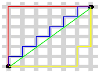
[image:1.595.342.511.579.705.2]

The distance is usually associated with an amount of distance that has to be covered by the taxis in Manhattan, because of their grid layout throughout the city.

Fig 1 Comparison of Manhattan and Euclidean Distances

In Fig 1, the comparison of the Manhattan and Euclidean distances has been indicated,

Juxtaposition of Different Machine Learning

Techniques for Improved Time Series

Classification

where the green line being the Euclidean distance, and others are Manhattan distance (MD) [4]. The equation to compute Manhattan distance is as stated in (2).

1

n

i i

i

d X Y







 (2)

C. Gradient Boosting

Ensemble modelling refers to a method of constructing either two or higher models. The models are distinct and associated with each other. Further, the integration of outcomes into as a vector or a scalar for the purpose of increasing the performance of a classifier in terms of accuracy. Gradient Boosting is a type of ensemble modelling.

The principal reasons of the variance in real and model-predicted magnitudes boil down to a noise, as well as a bias. The ensemble model enables to lessen both of those parameters. The motive behind the usage of numerous distinctive predictors attempting to expect the identical goal response may do a superior function than any individual predictor. Moreover, the ensemble strategies are categorised into the Bagging and Boosting techniques. We will be discussing the Boosting model.

In Boosting model, the predictors are not independent but are sequential and are dependent on the error output from the previous predictor. The following error is used to train the current predictor, and hence

it has been pointed out that the a set of rows which possess uneven probability of occurance and with maximum error turn out the most [9].

Gradient boosting and XGBoosting are examples of boosting algorithm. We have used XGBoosting for training our model. We chose XGBoosting because of its additive combining property, which reduces the bias of the dataset while keeping the variance low. The below example is an Illustration of the effect of different regularization strategies for Gradient Boosting, which shows that various combinations with stochastic gradient boosting and shrinkage can produce more accurate models by reducing the variance.

Fig.3. Visualization of Test Set Deviance w.r.t. Boosting Iterations

In Fig.3, the blue curve is the first subsample, without any learning rate, while the grey and pink ones are the subsequent curves after the first stage of gradient boosting. This shows the efficiency of regularization while getting the test set deviance to a minimal value. The dataset used for this example was CBF from UCR time series datasets [8].

D. Logistic regression

Logistic regression (LR) is employed whilist the response feature is categorical. It computes the representation using a mathematical formula, where input vectors (p) for a linear combination with the coefficient weights to yield the output (q). A significant variation of linear regression is a logistic regression where the output (q) has assigned a binary outcome instead of a set of continuous numerals. The illustrative logistic regression equation as indicated in (4).

0 1

0 1

( ) ( )

1 p

p

e q

e

 

 







 (4)

Here, the output of logistic regressor is denoted by q. The

0

 stands for intercept value, in addition ₀ reflects the

coefficient corresponding to input vector p [10]. The model which is preserved in computer‟s memory contains the values of coefficients of (4).

E. Piecewise Aggregate approximation

Commonly, time-series datasets and databases favour growing to substantial sizes. Sampling continuously is a call for in a ramification of instances in which those databases are concerned. throughout this manner, the capacity to head searching through the database will become unreasonably time-consuming. One algorithm that assists in executing those searches quickly and effectively is the PAA addressed in Keogh et al. [14]. The simple idea following the algorithm is:

Perform lessening of the input vector time series dimensions with division of them into equal-sized fragments which are computed by averaging the values in these fragments. Below is an example of PAA on ECG200 Dataset from UCR time series dataset [8].

Fig.4. The PAA transformation of raw data In Fig.4, the curve with the red colour represents the PAA transformation of the original data, which is represented in the background with blue colour. The number of segments in which the data has been divided is 10.

PAA tends to another representation called Symbolic Aggregate approXimation, shortened to SAX(Explained in the next section). This takes the lessen dimensionality and assigns a string representation to the graph. By providing a string illustration, the combination information this is to be stored less than different facts mining techniques, Eg. Discrete Fourier transform and Wavelet Transformation. The publicity comes from looking to examine and cluster, as an instance, strength intake statistics sampled every 15 minutes. via breaking the profiles into daily cycles and approximating it offers a quick assessment on

amassed, i.e., hastens the system of similarity searches and evaluation towards other profiles the use of Euclidean distance measures [12].

F. Support Vector Machine

Support vector machine (SVM) algorithm has been a part of the supervised machine learning algorithms, which has been employed to both regression and classification problems. Though, in general its utilized for classification intricacies. In present context, we visualize the object as a factor in m-D vector space (wherein „m‟ stands for variety of features). Subsequently, we do category with the aid of locating the hyperplane that differentiates the two classes thoroughly. Hence, it is clear that SVM is a discerning classifier usually indicated with the help of separating hyperplanes. There are several parameters involved while classification using SVM. They are; Regularization parameter (C parameter), gamma and the kernel used. We have utilized sci-kit learn library [7] to apply classification using SVM. The classification heavily depends on its parameters. These parameters need to be set according to the dataset we are dealing with; this step is termed as parameter tuning.

G. 1NN Classification

1NN classification algorithm lies under the k Nearest neighbour classifier, which is also known as sluggish machine learning technique because this algorithm will not optimize the objective mapping reflections of the training data. However, it tries to "remember" the training dataset. It is an instance-based classification technique.

The classification considers the distance similarity metric as a performance measure which predicts the labels of the test dataset. This classification algorithm is one of the oldest known classification methods, and yet it is very hard to beat convincingly when used with DTW.

kNN algorithm:

 To split the data into test and train datasets.

 Finds the k nearest neighbour (s) to any point „X_q‟

which is the assigned query point.

 The labels of all those nearest points are then stored.

 The query point class is subsequently assigned with the help of majority voting algorithm, from the stored labels.

For 1NN the algorithm is same, the only difference is the 1st nearest neighbour from the query point is considered, and hence the label corresponding to that neighbour is the predicted label.

H. Symbolic aggregate approximation

As mentioned in the above section, PAA is used to form another representation technique, which is SAX. We will use the same dataset to demonstrate the working of SAX as we did in PAA, in the previous section.

In laymen term, SAX representation is obtained by first converting the time series to PAA representation and then convert PAA to symbols.The use of PAA brings benefits of a easy and green dimensionality reduction whilst supplying the critical bottom limiting assets. The actual transformation of PAA coefficients toward letters via the use of a studies table is likewise computationally coherent.Digitization of Piecewise Aggregate Approximation, instantiation of time-collection toward Symbolic Aggregate Approximation is carried out significantly that yields respective symbols for the time-series

with the same probability. The vast and stringent assessment of numerous time-series datasets is accessible with proper set of rules. The authors performed the experimentation to indicate the amplitudes of „z normalized‟ time-collection comply with the ordinary spreading. Via the use of its residues, it is smooth to capture identical-looking regions beneath the standard curve with the help of lookup tables to reduce traces values, reducing below the Gaussian curve vicinity. Below in Fig.5 is the SAX representation with 10 PAA segments and 5 SAX breakpoints, on ECG200 Dataset.

Fig.5. SAX representation I. WEASEL

WEASEL stands for Word ExtrAction for time Series cLassificaion, in which it utilizes sliding windowing technique to yield a set of feature vectors which further is analyzed using a machine learning model of choice. In this work, we will address with the outcomes with various combinations of machine learning models with different features. WEASEL has been proven to be better in accuracy in the order of magnitude, even better than the current non-ensemble models and is almost as accurate as an ensemble classifier.[15]

The working of WEASEL consists of:

 Windowing of time series which gives us discriminative Fourier values. ANOVA F-Test aids this.

 From the Discriminative Fourier values,

discriminative words are extracted using supervised quantization (Information gain).

 First, if all the co-occurring words are used for making the bigrams of multiple window lengths.

 Discriminative features are then selected using CHI squared feature selection.

This concludes the whole pipeline of WEASEL, which refers to supervised symbolic representation in the first two points and Bag of patterns technique in the latter points.[15

J. Dynamic Time Warping

Dynamic time warping (DTW) represents a time series analysis algorithm which

processes the degree of similarity between two progressive sequences [5]. In laymen term, DTW finds the optimal match between any two given courses, with some restrictions and rules. As the previous distances have some disadvantage, that is they are susceptible to even a small mismatch among two available time series, such as, if

moved version of first time series however in other sense they are identical, thus the Euclidean or Manhattan distance amongst the both would be irrationally high. DTW overcomes the above shortcomings efficiently.

DTW algorithm and example:

Given the two-time series A and B , DTW distance is computed by first finding the best alignment between them. To align the two-time series, an n m matrix is constructed whose ( th

i , _jth _{) element is equal to (}

i j

a b ) which represents the cost to align the point a_iof time seriesAwith the point b_jof time seriesB. An alignment between the two time series is represented by a warping path, P =

1, 2, 3,..., k,..., K

p p p p p , in the matrix that governs the

following characteristics: adjoining and either constant or increasing. It begins with the bottom-left region and concludes on the top-right coordinate of the DTW matrix. A warping path then gives the best alignment over the DTW matrix. This calculation optimizes the overall point-alignment cost, thus respective optimal overall cost is denoted by the term „DTW-distance‟. Therefore, the equation for DTW will be as stated in (3).

2

1, ( , ) 1 2 3

arg min

( , ) ( )

, , ,..., ,..., k

P

K

i j k p i j k K

DTW A B a b

P p p p p p  

 







(3)

We have used NumPy library to create an example of DTW algorithms working; the code for this example is available at [6]. We chose to have two randomly generated arrays which are x and y, used Euclidean distance as the distance norm in this demonstration, to aid in finding the DTW similarity matrix or the cost matrix. Then by utilizing the properties of matplotlib, we plotted the best path in the cost matrix, as shown in Fig. 2.

Fig.2. Cost matrix and best path

DTW has been widely used as a similarity measure with numerous machine learning algorithms. We will be using DTW and DTW distance matrix later in this paper.

K. Using distances as a feature

As mentioned before, various distances and similarity measures are used for training different machine learning models, has been a conventional way of training statistical learning models. In this work, we have referred to way of using the distance matrix of various distances as a feature [1]. All the representation are feature-specific representations which are obtained and provided to the statistical learning algorithm while undergoing training process. The main advantage of using feature-based representations are we can

concatenate to feature matrix to form a single feature matrix. [1]

III. EXPERIMENT

This section consists of a brief about experimentation methodologies and the roadmap of our findings. This part explains the concepts used for doing these tasks.

A. Preprocessing of the datasets

The UCR time-series datasets are formed in such a manner wherein each dataset the first column has the class labels of each row, and the rest is the data. So, first, we need to divide the data into labels and features. After that, we can use the data for making the distance matrix using different distances or can use as a feature to train our machine learning models. This was done by simple slicing using Pandas and NumPy libraries.

B. Building the feature matrix

While building the feature matrix, the feature representation of time series is its respective distance from the training example.

Fig.6. Mechanism to build a feature matrix Fig.6 is a visual depiction of the mechanism to build the feature matrix where the feature train matrix is made by finding the distances between the train x train dataset, and the feature test matrix is formed between train x test dataset.[1] “Feature train” and “Feature Test” are the new features which are in turn provided to the state of the art machine learning models for training purpose. The Dark and light blue boxes are Train and Test labels, respectively. These colour conventions will continue all along with the paper. In a similar manner, we can build feature matrices using MD, ED, DTW Distances as a distance measure.

C. Using SAX and PAA as a feature

[image:5.595.309.516.53.362.2]

Fig.7. Matrix description

Fig.8. Distance of represented matrices

Fig. 7 describes the matrices, which has the representations of the Train and Test datasets. This is further used as a feature matrix for machine learning models. While the figure showed a SAX representation technique, one can also use PAA or any other representation technique. Fig. 8 shows how we can use the distance of the represented matrices, which has a similar order of finding the feature matrices as mentioned before in the paper. Hence, using any representation as a feature, we must use the transformed dataset as a feature, and as per the distance matrices, they must be calculated from their respective training representation datasets.

D. Feature concatenation

One of the best highlights of this method is its versatility for any representation method, which means we can concatenate different feature matrices and then can use it to train the machine learning models. We will be discussing some of the restrictions and procedures on how to concatenate two feature matrices.

The feature concatenation is simple horizontal concatenation, where each feature matrix must have the same number of rows as its respective label matrix has. This was ensured by resizing each feature matrix after its formation. We can use different distance or representation matrices, concatenate them and then they would be utilized in the form of a feature matrix for training machine learning models.

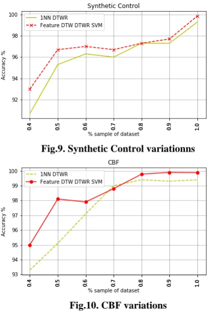
E. Change in accuracy over the varying lengths of a time series.

The change in accuracy over the varying length of time series was done to examine the accuracy trend over different samples of time series. This showed us the nature of the time series accuracies when we vary the time series length. This also acknowledges the random nature of the datasets, plus their behaviour over the entire time series. Below are some observed graphs of accuracies over different time series length on CBF and Synthetic Control datasets.

Fig.9. Synthetic Control variationns

Fig.10. CBF variations

Fig 9,10 shows the accuracy trend over different samples of time series. We can clearly see the increasing accuracy as the time series length has been increased. This also shows how the concatenated features used with SVM gives better accuracies as compared to 1NN DTWR combination.

F. Using different classification techniques

We have used different machine learning classifications with different sets of features. This was to find the best combination of classification technique with its respective dataset, considering the type of dataset. The 1NN classification was set to be the reference technique, with DTW distances as a similarity measure. In total, we have used five classification algorithms which are Nearest neighbours, Support Vector Machine, Gaussian process, Gradient Boosting and Logistic Regression. We will find the best combination among them in the following sections.

G. Resources used

The code is written in Python and the resources used in this experimentation setup are all Python libraries namely:

 Tslearn

 Pandas

 NumPy

 Pyts

 Matplotlib

 Sklearn

 Xgboost

H. Dataset Details

The dataset we used is UCR time series dataset [8] which has a variety of datasets. We have used various types of datasets for our experiment as per to

[image:5.595.58.253.66.260.2]

classifiers with different classifiers for different datasets. First column of the dataset is the classes assigned to the temporal data which is being used as the labels, the rest of the columns are used as the features to train our built models.

IV. RESULTS

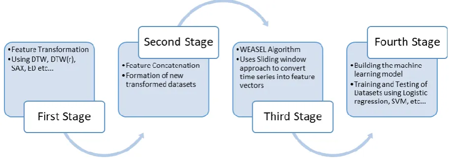
The approach in this paper was to converge the properties of feature transformation and concatenation and use it with a new approach to find more accurate predictions. We used Distance time warping and its different variants to transform the given dataset. For clarification the below explanation is distributed different stages, which concludes the whole process of experimentation performed. The flow diagram for the proposed approach is indicated in Fig.11.

First Stage: The feature transformation, we used different techniques – DTW, DTW(r), SAX, PAA, Euclidean distance and Manhattan Distance – for feature transformation. The transformation process was to compute the aforementioned similarity measures and distances and construct a matrix out of it. Second Stage: After transformation, the next step was to concatenate the transformed features matrices into a single matrix, which will then be used as the Train/Test dataset for further operations. Third Stage: The involvement of WEASEL Algorithm, which is a state-of-the-art method which transforms the time series (Dataset) into feature vectors.

Fourth Stage: Building and training of the model, where we use different Machine learning techniques, to train and test the transformed datasets. This also includes hyperparameter tuning depending on the type of the dataset we are working on. After using each and every classification algorithm and dataset combination, as aforementioned in the paper, we would be showing the list of accuracies for different

[image:6.595.68.525.486.651.2]

time-series datasets. The below Table 1 shows the list of accuracies of 29 datasets used for the experiment. Table 2 shows the various comparisons between the best methods picked from the 49 iterations done. Each cell within the table indicates on what number of datasets did the classifier in its row (Win, lose, tie) over the classifier in its column. The symmetric reproduction comparisons were left out for better understanding. The results shown in bold are the ones who tell us which are the methods giving most win over tie/loss and hence categorizes the best methods (column-wise). According to Table 2, Feature DTW_DTWR_ED_MD, WEASEL LR and Feature DTW_DTWR_ED_WEASEL_LR are the better-performing methods. Out of these three methods, we will now compare these results with results of classification method of 1NN DTW.

Fig.11. Proposed Time series classification work flow diagram

[image:7.595.74.527.56.211.2]

Table 1

Type Name Train Test Class Length Warping window ED (w=0) DTW (learned_w) DTW (w=100) MD SVM ED SVM DTW SVM DTWR SVM Feature DTW_DTWR_ED_MD_SVMFEATURE ALL SVM PAA_DIST_SVM WEASEL FEATURE_DTW_DTWR_ED WEASEL Image Adiac 390 391 37 176 3 0.389 0.391 0.396 0.361 0.389 0.335 0.361 0.353 0.448 0.394 0.261 0.389 Spectro Beef 30 30 5 470 0 0.333 0.333 0.367 0.367 0.333 0.4 0.433 0.367 0.467 0.367 0.167 0.433 Sensor Car 60 60 4 577 1 0.267 0.233 0.267 0.367 0.317 0.4 0.367 0.317 0.35 0.35 0.267 0.367 Simulated CBF 30 900 3 128 11 0.148 0.004 0.003 0.067 0.122 0.003 0.023 0.006 0.01 0.047 0.311 0.011 ECG ECG200 100 100 2 96 0 0.12 0.12 0.23 0.12 0.12 0.18 0.11 0.1 0.11 0.12 0.26 0.21 Image FacesUCR 200 2050 14 131 12 0.231 0.088 0.095 0.207 0.241 0.149 0.136 0.156 0.144 0.282 0.415 0.198 Motion GunPoint 50 150 2 150 0 0.087 0.087 0.093 0.053 0.047 0.067 0.08 0.047 0.087 0.067 0.04 1 Spectro Ham 109 105 2 431 0 0.4 0.4 0.533 0.295 0.333 0.324 0.305 0.324 0.324 0.314 0.295 0.314 Image Herring 64 64 2 512 5 0.484 0.469 0.469 0.406 0.359 0.5 0.484 0.469 0.438 0.406 0.391 0.5 Spectro Meat 60 60 3 448 0 0.067 0.067 0.067 0.1 0.4 0.517 0.417 0.1 0.3 0.417 0.117 1 Sensor MoteStrain 20 1252 2 84 1 0.121 0.134 0.165 0.108 0.128 0.212 0.125 0.144 0.158 0.22 0.142 0.177 Spectro OliveOil 30 30 4 570 0 0.133 0.133 0.167 0.2 0.6 0.6 0.6 0.2 0.6 0.6 0.133 0.3 Sensor Plane 105 105 7 144 5 0.038 0 0 0.029 0.019 0.038 0.038 0.019 0.019 0.019 0.019 0.038 Spectro Strawberry 613 370 2 235 0 0.054 0.054 0.06 0.038 0.051 0.062 0.041 0.041 0.065 0.054 0.03 0.076 Simulated SyntheticControl 300 300 6 60 6 0.12 0.017 0.007 0.023 0.037 0.013 0.017 0.013 0.017 0.057 0.12 0.02 ECG TwoLeadECG 23 1139 2 82 4 0.253 0.132 0.096 0.347 0.277 0.13 0.299 0.337 0.293 0.341 0.299 1 Spectro Wine 57 54 2 234 0 0.389 0.389 0.426 0.185 0.5 0.5 0.5 0.204 0.5 0.5 0.167 0.389 Simulated UMD 36 144 3 150 4 0.236 0.028 0.007 0.076 0.076 0.042 0.16 0.021 0.014 0.104 0.292 0.035 Spectro Coffee 28 28 2 286 3 0 0 0 0.071 0 0.036 0.036 0.071 0.036 0 1 1 Motion CricketX 390 390 12 300 7 0.423 0.228 0.246 0.364 0.459 0.31 0.321 0.3 0.3 0.413 0.549 0.315 Motion CricketY 390 390 12 300 17 0.433 0.241 0.256 0.377 0.444 0.305 0.328 0.282 0.272 0.49 0.564 0.313 Motion CricketZ 390 390 12 300 7 0.413 0.254 0.246 0.346 0.438 0.308 0.297 0.287 0.287 0.415 0.49 0.279 Image DiatomSizeReduction 16 306 4 345 0 0.065 0.065 0.033 0.082 0.072 0.101 0.098 0.082 0.095 0.078 0.173 0.065 Image FaceAll 560 1690 14 131 3 0.286 0.192 0.192 0.272 0.26 0.136 0.238 0.253 0.17 0.299 0.202 0.168 Image FaceFour 24 88 4 350 2 0.216 0.114 0.171 0.17 0.205 0.17 0.205 0.193 0.193 0.205 0.534 0.239 Sensor ItalyPowerDemand 67 1029 2 24 0 0.045 0.045 0.05 0.044 0.036 0.077 0.072 0.041 0.091 0.098 0.077 0.041 Sensor Lightning2 60 61 2 637 6 0.246 0.131 0.131 0.295 0.311 0.164 0.377 0.295 0.164 0.262 0.459 0.279 Sensor Lightning7 70 73 7 319 5 0.425 0.288 0.274 0.26 0.301 0.288 0.356 0.178 0.219 0.356 0.534 0.288 Image MedicalImages 381 760 10 99 20 0.316 0.253 0.263 0.282 0.303 0.286 0.271 0.234 0.276 0.313 0.379 0.247

In Table 1 we can visualize that 1NN DTWR, Feature ED MD DTW DTWR, WEASEL, AND Feature ED MD DTW DTWR WEASEL are for combinations which yields lesser error rates consistently as compared to other combinations.

Table 2: Consists of various comparison between the best methods picked from the 49 iterations done. All comparisons are done using 29 UCR time series classification datasets. The outcomes indicated in the bold face font are the ones which tells us which are the methods giving most win over tie/loss and hence categorizes the best methods (column wise).

Table 2

Methods ED SVM DTW SVM DTWR SVM Feature DTW_DTWR_ED_MD Feature DTW_DTWR_ED_SAX_SVM Feature PAA_Dist_SVM WEASEL Feature DTW_DTWR_ED_WEASEL_LR

MD SVM (17, 10, 2) (16, 12, 1) (16, 11, 2) (6, 17, 6) (13, 16, 0) (19, 7, 3) (17, 11, 1) (16, 12, 1)

ED SVM - (12, 15, 2) (13, 13, 3) (7, 19, 3) (11, 15, 3) (18, 5, 6) (18, 10, 1) (13, 15, 1)

DTW SVM - - (13, 12, 4) (8, 19, 2) (10, 14, 5) (16, 10, 3) (16, 12, 1) (16, 10, 3)

DTWR SVM - - - (6, 22, 1) (9, 15, 5) (15, 9, 5) (16, 12, 1) (13, 13, 3)

Feature DTW_DTWR_ED_MD - - - - (16, 8, 5) (22, 5, 2) (16, 12, 1) (23, 5, 1)

Feature DTW_DTWR_ED_SAX_SVM - - - (17, 8, 4) (16, 12, 1) (19, 10, 0)

Feature PAA_Dist_SVM - - - (14, 14, 1) (12, 16, 1)

WEASEL - - - (13, 15, 1)

Observing Table 2, we can conclude Feature DTW_DTWR_ED_MD, WEASEL and Feature

DTW_DTWR_ED_WEASEL_LR are the three best performing methods out these 9 methods.

Table 3 shows the time taken by each of them to compute the output, with training and testing time, respectively. Table 3

Combination

Training time Testing time

1NN DTWR

128 m 20 s

322 m 44s

Feature DTW_DTWR_ED_MD_SVM

488 m 33 s

1332 m 02s

Feature DTW_DTWR_ED_MD_WEASEL LR

139 m 55s

278 m 09s

WEASEL LR

2m 43s

233m 18s

Hence, we can see WEASEL LR (logistic regression) takes the minimum time followed by Feature DTW DTWR ED MD WEASEL LR. Feature DTW DTWR ED MD with SVM takes maximum time. The next part consists of the graph (Fig 3.1),

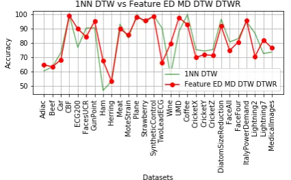
[image:7.595.320.533.567.699.2]

which compares Feature DTW DTWR ED MD WEASEL LR with the rest of the methods.

Fig.12. 1NN DTW vs Feature DTW_DTWR_ED_MD_WEASEL

[image:7.595.65.272.567.700.2]

[image:8.595.65.272.53.179.2]

Fig.14. 1NN DTW vs WEASEL

Fig 12 shows that the method has 16 out of 29-win cases out of all the methods applied. This result was obtained in the time of 418 minutes and 4 seconds. This result was followed by Fig 13 and Fig 14, where we can visualize there are 16- and 12-win cases respectively.

[image:8.595.314.538.101.432.2]

After this comparison we will compare these results with the results of Feature SAX-DTW-DTWR as mentioned in [1].

Fig.15. Feature SAX-DTW-DTWR vs Feature DTW_DTWR_ED_MD_SVM

Fig.16. Feature SAX-DTW-DTWR vs FEATURE_DTW_DTWR_ED_WEASEL

Fig.17. Feature SAX-DTW-DTWR vs WEASEL Fig 15-17 are the comparisons from the Feature SAX-DTW-DTWR, which is the best method as mentioned in

[1]. Here we can see that WEASEL and Feature ED-MD-DTW-DTWR-SVM are the closest approaches which resembles the results. They have 10 out of 29 and 16 out of 29-win cases.

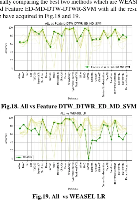
Finally comparing the best two methods which are WEASEL and Feature ED-MD-DTW-DTWR-SVM with all the results we have acquired in Fig.18 and 19.

Fig.18. All vs Feature DTW_DTWR_ED_MD_SVM

Fig.19. All vs WEASEL LR V. CONCLUSION

[image:8.595.59.272.246.740.2]

REFERENCES

1. Kate, Rohit J. "Using dynamic time warping distances as features for improved time series classification." Data Mining and Knowledge Discovery 30.2 (2016): 283-312.

2. Abanda, Amaia, Used Mori, and Jose A. Lozano. "A review on distance based time series classification." Data Mining and Knowledge Discovery 33.2 (2019): 378-412.

3. Dau, Hoang Anh, et al. "The UCR time series archive." arXiv preprint

arXiv:1810.07758 (2018).

4. Krause EF. Taxicab geometry: An adventure in non-Euclidean

geometry. Courier Corporation; 1986.

5. Berndt, Donald J., and James Clifford. "Using dynamic time warping

to find patterns in time series." KDD workshop. Vol. 10. No. 16. 1994. 6. Ishan Yash. (2019, July 19). ishanyash/DTW-Example: Test release of

my work (Version v1.0.0). Zenodo. http://doi.org/10.5281/zenodo.3343058

7. Scholkopf B, Smola AJ. Learning with kernels: support vector

machines, regularization, optimization, and beyond. MIT press; 2001 Dec 1.

8. Hoang Anh Dau, Eamonn Keogh, Kaveh Kamgar, Chin-Chia Michael Yeh, Yan Zhu, Shaghayegh Gharghabi , Chotirat Ann Ratanamahatana,Yanping Chen, Bing Hu, Nurjahan Begum, Anthony Bagnall , Abdullah Mueen and Gustavo Batista (2018). The UCR Time Series Classification Archive. URL https://www.cs.ucr.edu/~eamonn/time_series_data_2018/

9. Chen, Tianqi, and Carlos Guestrin. "Xgboost: A scalable tree boosting system." Proceedings of the 22nd acm sigkdd international conference on knowledge discovery and data mining. ACM, 2016.

10. Hastie, Trevor, Robert Tibshirani, and Jerome Friedman. "The elements of statistical learning: data mining, inference, and prediction, Springer Series in Statistics." (2009): xxii-745.

11. Lin, J., Keogh, E., Patel, P., and Lonardi, S., Finding Motifs in Time Series, The 2nd Workshop on Temporal Data Mining, the 8th ACM Int' l Conference on KDD (2002)

12. Patel P, Keogh E, Lin J, Lonardi S. Mining motifs in massive time series databases. In2002 IEEE International Conference on Data Mining, 2002. Proceedings. 2002 Dec 9 (pp. 370-377). IEEE. 13. Keogh, E., Lin, J. and Fu, A., 2005, November. Hot sax: Efficiently

finding the most unusual time series subsequence. In Fifth IEEE International Conference on Data Mining (ICDM'05) (pp. 8-pp). Ieee. 14. Keogh E, Chakrabarti K, Pazzani M, Mehrotra S. Dimensionality reduction for fast similarity search in large time series databases. Knowledge and information Systems. 2001 Aug 1;3(3):263-86. 15. Schäfer, Patrick, and Ulf Leser. "Fast and accurate time series

classification with weasel." Proceedings of the 2017 ACM on Conference on Information and Knowledge Management. ACM, 2017.

AUTHORSPROFILE

Ishan Yash, Final year undergraduate student from VIT Vellore, Pursuing Electronics engineering with a specialization in Internet of Things and sensors. An aspiring engineer who is interested in data science and analytics.

Dr. Hemprasad Yashwant Patil is presently working at Vellore Institute of Technology, Vellore, India as Assistant Professor. He has completed Ph.D. from VNIT Nagpur in 2015. He has published more than 20 research articles in reputed journals and conferences in the domain of Image processing, Deep learning, Machine learning and computer vision. He also serves as a reviewer to journals like IEEE Transactions on Information Forensics and Security, Neurocomputing etc.

Dr. Usha Rani Seshasayee is with Vellore Institute of Technology, Vellore, India as Senior Assistant Professor, since November 2018. She has eight years of experience, each in Industry and Teaching. She has obtained her doctoral degree from IIT Madras in the area of Performance analysis of Communication