Optimized schwarz methods for Maxwell equations with discontinuous coefficients

Equations with Discontinuous Coefficients

Victorita Dolean1, Martin J. Gander2, Erwin Veneros3

1 Introduction

After the development of optimized Schwarz methods for the Helmholtz equation [2, 3, 4, 12, 14], extensions to the more difficult case of Maxwell’s equations were developed: for curl-curl formulations, see [1]. For first order formulations without conductivity, see [7], and with conductivity, see [5, 11]. For DG discretizations of Maxwell’s equations, optimized Schwarz methods can be found in [6, 8, 9], and for scattering problems with applications, see [15, 16].

We present here optimized Schwarz methods for Maxwell’s equations in hetero-geneous media with discontinuous coefficients, and show that the discontinuities need to be taken into account in the transmission conditions in order to obtain effec-tive Schwarz methods. For diffusive problems, it was shown in [10] that jumps in the coefficients can actually lead to faster iterations, when they are taken into account correctly in the transmission conditions. We show here that for the case of Maxwell’s equations with jumps along the interfaces, one can obtain a non-overlapping opti-mized Schwarz method that converges independently of the mesh parameter; this is not possible without coefficient jumps.

2 Schwarz Methods for Maxwell’s Equations

The time dependent Maxwell equations are

−ε∂E

∂t +∇×H =J, µ ∂H

∂t +∇×E =0, (1)

whereE = (E1,E2,E3)T is the electric field,H = (H1,H2,H3)T is the magnetic field, ε is theelectric permittivity, µ is themagnetic permeability, andJ is the applied current density. We assume that the applied current density is divergence free, divJ=0.

The time dependent Maxwell equations (1) are a system of hyperbolic partial dif-ferential equations, see for example [7]. This hyperbolic system has for any interface two incoming and two outgoing characteristics. Imposing incoming characteristics is equivalent to imposing the impedance condition

Section de math´ematiques, Universit´e de Gen`eve, 1211 Gen`eve 4

[email protected] · [email protected] ·

[email protected]

Bn(E,H):=E

Z ×n+n×(H ×n) =s. (2)

We consider in this paper the time-harmonic Maxwell equations,

−iω εE+∇×H=J, iω µH+∇×E=0, ∈Ω, (3)

and study the heterogeneous case where the domainΩconsists of two non-overlapping subdomainsΩ1andΩ2with interfaceΓ, with piecewise constant parametersεjand

µjinΩj,j=1,2. A general Schwarz algorithm for this configuration is

       

      

−iω ε1E1,n+∇×H1,n=J inΩ1, iω µ1H1,n+∇×E1,n=0 inΩ1, (Bn1+S1Bn2)(E

1,n_,H1,n_{) = (B}

n1+S1Bn2)(E

2,n−1_,H2,n−1_{) on} Γ, −iω ε2E2,n+∇×H2,n=J inΩ2,

iω µ2H2,n+∇×E2,n=0 inΩ2, (Bn2+S2Bn1)(E

2,n_,H2,n_{) = (B}

n2+S2Bn1)(E

1,n−1_,H1,n−1_{) onΓ,} (4)

whereSj, j=1,2 are tangential, possibly pseudo-differential operators, and

Bnj(E

j,n_,Hj,n_{) =}Ej,n

Zj

×n_j+n_j×(Hj,n×n_j)

with Zj=

p

µj/εj, j=1,2. Different choices of Sj, j=1,2 lead to different

Schwarz methods [7].

3 The Classical Schwarz Method

The classical Schwarz method is exchanging characteristic information at the inter-faces between subdomains, which means Sj =0. For the case of discontinuous

coefficients and the domain Ω =R3, with the Silver-M¨uller radiation condition limr→∞r(H×n−E) =0, and the two subdomainsΩ1= (−∞,0)×R2, Ω2=

(0,∞)×R2, the classical Schwarz method does not converge in the presence of co-efficient jumps:

Theorem 1.For any(E1,0,H1,0)∈(L2(Ω1))6and(E2,0,H2,0)∈(L2(Ω2))6, ifµ1ε26= µ2ε1the classical Schwarz algorithm diverges in(L2(Ω1))6×(L2(Ω2))6.

Proof. Performing a Fourier transform in theyzplane with Fourier variablesk:= (ky,kz),|k|=ky2+kz2, we obtain after a lengthy calculation similar to the one found

in [7] the convergence factor

ρcla(k,ω1,ω2,Z) =max{ρ1(k,ω1,ω2,Z),ρ2(k,ω1,ω2,Z)}

withω1=ω√ε1µ1,ω2=ω√ε2µ2,Z= q

µ1ε2

ρ1(k,ω1,ω2,Z) = q

|k|2_−ω2 1−iω1Z

q

|k|2_−ω2

2−iω2/Z

q

|k|2_−ω2 1+iω1

q

|k|2_−ω2 2+iω2

1 2 , (5)

ρ2(k,ω1,ω2,Z) = q

|k|2_−ω2

1−iω1/Z q

|k|2_−ω2 2−iω2Z

q

|k|2_−ω2 1+iω1

q

|k|2_−ω2 2+iω2

1 2 . (6)

The conditionµ1ε26=µ2ε1is equivalent toZ6=1. To show divergence, we consider 3 cases: ifω1>ω2, we obtain for|k|=ω1

ρ₁4(k,ω1,ω2,Z) =1+(ω 2

1−ω22)(Z2−1) ω₁2

, ρ₂4(k,ω1,ω2,Z) =1−(ω 2

1−ω22)(Z2−1) ω₁2Z2

,

and hence ifZ>1 we haveρ2>1, and ifZ<1 we haveρ1>1. Therefore, the algorithm diverges forω1>ω2. Similarly ifω1<ω2we get for|k|=ω2

ρ₁4(k,ω1,ω2,Z) =1− (ω2

2−ω12)(Z2−1) ω₂2Z2 ρ

4

2(k,ω1,ω2,Z) =1+ (ω2

2−ω12)(Z2−1) ω₂2

,

and we obtain divergence as in the first case. Finally, ifω1=ω2, we find

ρ1(k,ω1,ω2,Z) =ρ2(k,ω1,ω2,Z) = q

|k|2_−ω2 1−iω1Z

q

|k|2_−ω2

1−iω1/Z

q

|k|2_−ω2 1+iω1

2

1/2 .

Setting now|k|=√2ω1, we get after some simplifications that

ρ₁4=1 4

(Z2+1)2 Z2 , andρ₁4>1 is equivalent to

ρ₁4>1 ⇐⇒ (Z2+1)2>4Z2 ⇐⇒ (Z2−1)2>0,

which always holds, because by assumptionZ6=1. So we also have divergence for the caseω1=ω2. ut

The case of continuous coefficients is analyzed in [7]. In this case,ρ1=ρ2, and ρcla(|k|)<1 for the propagative modes,|k|<ωj, j=1,2, andρcla(|k|) =1 for the

evanescent modes,|k|>ωj, j=1,2, so the algorithm is stagnating for all

evanes-cent modes. This is also the case ifµ1ε2=µ2ε1which was excluded in Theorem 1 .

ana-lyze now the special case of the two dimensional transverse magnetic (TMz) and transverse electric (TEz) Maxwell equations. In the TMz case, the unknowns are independent ofz, and we haveE= (0,0,Ez)andH= (Hx,Hy,0). In the TEz case,

E= (Ex,Ey,0)andH= (0,0,Hz). Since we obtain identical results in the TMz case

and the TEz case (one just has to exchange the roles ofεwithµ), we only show the TMz case. Our results are again based on Fourier transforms, here in theydirection with Fourier variablek. After a similar computation as in the proof of Theorem 1, we obtain for the classical Schwarz algorithm for the TMz case the convergence factor

ρcla(k,ω1,ω2,Z) =

q k2_−ω2

1−iω1Z q

k2_−ω2

2−iω2/Z

q k2_−ω2

1+iω1 q

k2_−ω2 2+iω2

1 2

. (7)

For the TMz formulation, the classical Schwarz algorithm can be convergent in the presence of coefficient jumps:

Theorem 2.Let µ1=µ2. Ifε1<ε2and q

ε1

ε2 >C0, or ifε1>ε2 and q

ε2

ε1 >C0, C0=0.3213357548..., then the classical Schwarz algorithm for the TMz case is convergent.

Proof. We can only give an outline of the proof: without loss of generality, we can assume thatω1<ω2. We then proceed in three steps: first, we show that for the evanescent modes,k>ωj, j=1,2 we haveρcla<1 ifε16=ε2. Second, we show

thatρclaatk=0 andk=ω1is strictly less than one, and finally we show that the maximum of those two values boundsρcla for all the propagative modesk<ωj,

j=1,2, where the restriction involvingC0comes in.

Theorem 3.Ifε1=ε2and µ16=µ2, then the classical Schwarz algorithm for the TMz case is divergent.

Proof. The proof is based on divergence of the evanescent modes, as in Theorem 1.

Theorem 4.Ifµ16=µ2,ε16=ε2and Z<

√

2

2 , then the classical Schwarz algorithm for the TMz case is divergent.

Proof. The proof is based again on divergence of the evanescent modes.

4 Optimized Schwarz Methods

c

S1=−s2−iω2Z

−1 s2+iω2

, S2c=−

s1−iω1Z s1+iω1

, (8)

then the optimized Schwarz method for the TMz case has the convergence factor

ρopt(ω1,ω2,µ1,µ2,s1,s2,k) = q k2_−ω2

1−s1 q

k2_−ω2 2−s2

q k2_−ω2

1+s2µµ12 q

k2_−ω2 2+s1µµ21

1 2 . (9)

In order to have a more efficient algorithm, we have to choose sj, j=1,2 such

that ρopt is as small as possible for all numerically relevant frequenciesk∈K:= [kmin,kmax], wherekminis a constant depending on the geometry andkmax=cmax/h, withcmaxa constant andhdenoting the mesh size, see for example [13]. We search forsj of the formsj=cj(1+i)such thatcj, j=1,2 will be the solutions of the

min-max problem

ρ∗= min

c1,c2≥0

max

k∈Kρopt(ω1,ω2,µ1,µ2,k,c1(1+i),c2(1+i))

. (10)

The proofs of the following theorems are based on asymptotic analysis, and are too long and technical for this short paper; they will appear elsewhere.

Theorem 5.Ifµ1<µ2and µ_µ2 1 >

√

2, and r=p|ε1µ1−ε2µ2|, then the asymptotic solution of the min-max problem for h small is

c∗₁=1 2

cmaxµ1(µ2+µ1−pµ2(4µ1+3µ2)) (µ2

2−2µ12)h

, c∗₂=ωr, (11)

ρ∗= 4 r

1 2−

23/4 4

ω(µ₂2−2µ₁2)r (µ2+2µ1−pµ2(4µ1+3µ2))

h+O(h2). (12)

If µ2

µ1 ≤ √

2, then the asymptotic solution of the min-max problem is

c∗₁= 1 2h

cmax(µ2−µ1)

µ2 , c

∗

2= ωrµ2

2 µ2+

q

2µ₁2−µ₂2

µ1−µ2 (13)

ρ∗= r µ1 µ2− r µ1 µ2 23/4

4

ωr(µ2+q2µ₁2−µ₂2) µ2−µ1 h+O(h

2_{). (14)}

Theorem 6.Ifµ1=µ2andε16=ε2, and r=p|ε1µ1−ε2µ2|, then the asymptotic solution of the min-max problem for h small is given by

c∗₁= cmax

h

3/4 ωr

2 1/4

, c∗₂=1₄2cmax

h

1/4

(ωr)3/4_{, (15)} ρ∗=1−(_2cωr

max)

Theorem 7.Ifµ1>µ2and µµ12 > √

2, and r=p|ε1µ1−ε2µ2|, then the asymptotic solution of the min-max problem for h small is

c∗₁=1 2

cmaxµ2(µ1+µ2−

p

µ1(4µ2+3µ1))

(µ₁2−2µ₂2)h , c ∗

2=ωr, (17)

ρ∗= 4 r

1 2−

23/4 4

ω(µ₁2−2µ₂2)r (µ₁+2µ2−

p

µ1(4µ2+3µ1))

h+O(h2), (18)

and if µ1

µ2 ≤ √

2then the asymptotic solution of the min-max problem is

c∗₁= 1 2h

cmax(µ1−µ2)

µ1

, c∗₂=ωrµ1 2

µ1+ q

2µ₂2−µ₁2

µ2−µ1 (19)

ρ∗= r

µ2

µ1 −

r µ2

µ1 23/4

4

ωr(µ1+ q

2µ₂2−µ₁2) µ1−µ2

h+O(h2). (20) Theorem 5 and Theorem 7 contain the surprising result that in the presence of jumps in the coefficients, it is possible to obtain an optimized Schwarz method for Maxwell’s equations with convergence factor that does not deteriorate when the mesh parameterhgoes to zero, even without overlap. In the first parts of each the-orem, we even see the convergence is independent of the jump in the coefficients. In the case ofµ1=µ2in Theorem 6 however, the convergence factor depends onh and deteriorates ashgoes to zero, as in the case in [7] when alsoε1=ε2.

5 Numerical Results

We now present some numerical results to illustrate the performance of the algo-rithms. We partition the domain Ω = (−1,1)×(0,1)into two subdomainsΩ1= (−1,0)×(0,1)andΩ2= (0,1)2. In each subdomain we select constant coefficients εj,µj, j=1,2. We discretize the TMz Maxwell’s equations using a finite volume

method, and we impose for the test on the outer boundary the impedance boundary condition _ZE

j×nj+nj×(H×nj) =0, j=1,2.

We first show in Figure 1 convergence histories for the classical Schwarz algo-rithm. On the left, we show in blue the case whenµ16=µ2andε1=ε2, and in red the case whenµ16=µ2andε16=ε2andZ<√1

2, and the algorithm diverges as pre-dicted by Theorem 3 and Theorem 4. On the right in Figure 1 we show in blue the case whenε16=ε2andµ1=µ2, and in red the case whenµ16=µ2andε16=ε2and Z>√1

2, and we observe convergence, as predicted by Theorem 2.

0 5 10 15 20 25 10−1

100

101

102

103 Graph of errors

err

2*iter e1=u1=1 e2=1 u2=5 e1=u1=1 e2=2 u2=5

0 5 10 15 20 25

10−3

10−2

10−1

100 Graph of errors

err

2*iter

e1=u1=1 e2=3 u2=1 e1=u1=1 e2=3 u2=2

Fig. 1 Convergence histories for the classical Schwarz algorithm. On the right two cases of

diver-gence, one whereεis continuous and one whereεis not continuous, and on the right two cases of convergence, one forµcontinuous and one forµnot continuous

10−2

101.4

101.5

101.6

101.7

h

iterations

Optimized Case 1 Optimized Case 2 Optmized Case 3

O(h−1/4₎

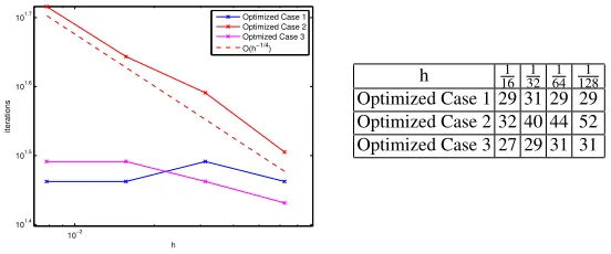
h ₁₆1 ₃₂1 ₆₄1 ₁₂₈1 Optimized Case 1 29 31 29 29 Optimized Case 2 32 40 44 52 Optimized Case 3 27 29 31 31

Fig. 2 Number of iterations against the mesh sizeh, to attain an error of 10−6_{with the 3 cases of}

the optimized Schwarz algorithm

whenhis refined. Clearly case 1 and 3 lead to convergence independent of the mesh size, as predicted by Theorem 5 and Theorem 7, whereas the convergence in case 2 deteriorates, as predicted by Theorem 6. We use here the parameters ω =2π, ε1=µ1=1 for all the cases. For the first case we setε2=2 andµ2=2, for the secondε2=2 andµ2=1 and for the thirdε2=1 andµ2=1.4<

√ 2.

6 Conclusions

conver-gence independent of the mesh parameter in the non-overlapping case, something which is impossible without coefficient jumps.

References

1. Alonso-Rodriguez, A., Gerardo-Giorda, L.: New nonoverlapping domain decomposition methods for the harmonic Maxwell system. SIAM J. Sci. Comput.28(1), 102–122 (2006) 2. Chevalier, P., Nataf, F.: An OO2 (Optimized Order 2) method for the Helmholtz and Maxwell

equations. In: 10th International Conference on Domain Decomposition Methods in Science and in Engineering, pp. 400–407. AMS (1997)

3. Despr´es, B.: D´ecomposition de domaine et probl`eme de Helmholtz. C.R. Acad. Sci. Paris

1(6), 313–316 (1990)

4. Despr´es, B., Joly, P., Roberts, J.: A domain decomposition method for the harmonic Maxwell equations. In: Iterative methods in linear algebra, pp. 475–484. North-Holland, Amsterdam (1992)

5. Dolean, V., El Bouajaji, M., Gander, M.J., Lanteri, S.: Optimized Schwarz methods for Maxwell’s equations with non-zero electric conductivity. In: Domain decomposition methods in science and engineering XIX,Lect. Notes Comput. Sci. Eng., vol. 78, pp. 269–276. Springer, Heidelberg (2011). DOI 10.1007/978-3-642-11304-8 30. URLhttp://dx.doi.org/ 10.1007/978-3-642-11304-8_30

6. Dolean, V., El Bouajaji, M., Gander, M.J., Lanteri, S., Perrussel, R.: Domain decom-position methods for electromagnetic wave propagation problems in heterogeneous me-dia and complex domains. In: Domain decomposition methods in science and engi-neering XIX, Lect. Notes Comput. Sci. Eng., vol. 78, pp. 15–26. Springer, Heidelberg (2011). DOI 10.1007/978-3-642-11304-8 2. URLhttp://dx.doi.org/10.1007/ 978-3-642-11304-8_2

7. Dolean, V., Gerardo-Giorda, L., Gander, M.: Optimized Schwarz methods for Maxwell equa-tions. SIAM J. Scient. Comp.31(3), 2193–2213 (2009)

8. Dolean, V., Lanteri, S., Perrussel, R.: A domain decomposition method for solving the three-dimensional time-harmonic Maxwell equations discretized by discontinuous Galerkin meth-ods. J. Comput. Phys.227(3), 2044–2072 (2008)

9. Dolean, V., Lanteri, S., Perrussel, R.: Optimized Schwarz algorithms for solving time-harmonic Maxwell’s equations discretized by a discontinuous Galerkin method. IEEE. Trans. Magn.44(6), 954–957 (2008)

10. Dubois, O.: Optimized Schwarz methods for the advection-diffusion equation and for prob-lems with discontinuous coefficients. Ph.D. thesis, McGill University (2007)

11. El Bouajaji, M., Dolean, V., Gander, M.J., Lanteri, S.: Optimized Schwarz methods for the time-harmonic Maxwell equations with damping. SIAM Journal on Scientific Computing

34(4), A2048–A2071 (2012). DOI http://dx.doi.org/10.1137/110842995

12. Gander, M., Magoul`es, F., Nataf, F.: Optimized Schwarz methods without overlap for the Helmholtz equation. SIAM J. Sci. Comput.24(1), 38–60 (2002)

13. Gander, M.J.: Optimized Schwarz methods. SIAM J. Numer. Anal.44(2), 699–731 (2006) 14. Gander, M.J., Halpern, L., Magoul`es, F.: An optimized Schwarz method with two-sided robin

transmission conditions for the Helmholtz equation. Int. J. for Num. Meth. in Fluids55(2), 163–175 (2007)

15. Peng, Z., Lee, J.F.: Non-conformal domain decomposition method with second-order trans-mission conditions for time-harmonic electromagnetics. J. Comput. Physics229(16), 5615– 5629 (2010). URLhttp://dx.doi.org/10.1016/j.jcp.2010.03.049

16. Peng, Z., Rawat, V., Lee, J.F.: One way domain decomposition method with second order transmission conditions for solving electromagnetic wave problems. J. Comput. Physics