Heterotic standard model moduli

      

City, University of London Institutional Repository

Citation

:

Braun, V., He, Y., Ovrut, B. A. and Pantev, T. (2006). Heterotic standard model moduli. Journal of High Energy Physics, 2006(JHEP01), 025 - 025. doi: 10.1088/1126-6708/2006/01/025

This is the unspecified version of the paper.

This version of the publication may differ from the final published

version.

Permanent repository link:

http://openaccess.city.ac.uk/859/

Link to published version

:

http://dx.doi.org/10.1088/1126-6708/2006/01/025

Copyright and reuse:

City Research Online aims to make research

outputs of City, University of London available to a wider audience.

Copyright and Moral Rights remain with the author(s) and/or copyright

holders. URLs from City Research Online may be freely distributed and

linked to.

City Research Online: http://openaccess.city.ac.uk/ [email protected]

arXiv:hep-th/0509051v3 25 Oct 2005

UPR 1131-T

hep-th/0509051

Heterotic Standard Model Moduli

Volker Braun

1,2

_{, Yang-Hui He}

1

_{, Burt A. Ovrut}

1

_{, and Tony Pantev}

2

1 _{Department of Physics,} 2 _{Department of Mathematics}

University of Pennsylvania Philadelphia, PA 19104–6395, USA

Abstract

In previous papers, we introduced a heterotic standard model and discussed its basic properties. The Calabi-Yau threefold has, generically, three K¨ahler and three complex structure moduli. The observable sector of this vacuum has the spectrum of the MSSM with one additional pair of Higgs-Higgs conjugate fields. The hidden sector has no charged matter in the strongly coupled string and only minimal matter for weak coupling. Additionally, the spectrum of both sectors will contain vector bundle moduli. The exact number of such moduli was conjectured to be small, but was not explicitly computed. In this paper, we rectify this and present a formalism for computing the number of vector bundle moduli. Using this formalism, the number of moduli in both the observable and strongly coupled hidden sectors is explicitly calculated.

Contents

1 Introduction 1

2 Preliminaries 3

2.1 The Calabi-Yau Threefold X . . . 3 2.2 The Observable Sector Bundle V . . . 4 2.3 Computing the Particle Spectrum . . . 6

3 The Exact Sequences 7

3.1 Short Exact Bundle Sequences . . . 7 3.2 Long Exact Cohomology Sequences . . . 8 3.3 The “Corner” Cohomologies . . . 9

4 The Long Exact Sequences 15

4.1 The H0 _{Cohomologies . . . . 15} 4.2 The H1 _{Cohomologies . . . . 17}

5 The Moduli 20

6 The Hidden Sector Moduli 20

A The Coboundary Map δ1 23

Bibliography 25

1

Introduction

There is a long history in the search for realistic compactifications of the heterotic string, see [1–19]. But until recently, finding compactifications yielding a viable particle spectrum had resisted all efforts. In a series of papers [20–22], we presented a “heterotic standard model” of particle physics. Specifically, we presented a small class of E8×E8 heterotic superstring vacua whose observable sectors have the spectrum of the minimal supersymmetric standard model (MSSM), with the exception of one additional pair of Higgs-Higgs conjugate superfields, andno exotic multiplets. Such vacua occur for both weak and strong string coupling.

Technically, our heterotic standard vacua consist of stable, holomorphic vector bun-dles, V, with structure group SU(4) over elliptically fibered Calabi-Yau threefolds, X, with a Z_3×Z_{3 fundamental group. These bundles admit a gauge connection that, in}

group down to theSU(3)C×SU(2)L×U(1)Y standard model group times an additional

U(1)B−L symmetry. The spectrum arises as the Z3×Z3 invariant sheaf cohomology. The existence of elliptically fibered Calabi-Yau threefolds withZ_{2 and}Z_2×Z₂

funda-mental group was first demonstrated in [23–25] and [26,27] respectively. More recently, elliptic Calabi-Yau threefolds with Z_3×Z_{3 fundamental group were constructed and}

classified [28]. Methods for building stable, holomorphic vector bundles with arbitrary structure group in E8 over simply connected elliptic Calabi-Yau threefolds were intro-duced in [29–32] and greatly expanded in a number of papers [23–25, 33–35]. These constructions were then generalized to elliptically fibered Calabi-Yau threefolds with non-trivial fundamental group in [25–27,36]. In order to obtain a realistic spectrum, it was found necessary to introduce a new method [23–27] for constructing vector bundles. This consists of building the requisite bundles by “extension” from simpler, lower rank bundles. This method was used for manifolds withZ_{2 fundamental group in [25,37,38]}

and in the heterotic standard model context in [28]. In recent work [20–22, 37, 38], it was shown how to compute the complete low-energy spectrum of such vacua. This requires one to evaluate the relevant sheaf cohomologies, find the action of the finite fundamental group on these spaces and, finally, to tensor this with the action of the Wilson line on the associated representation. The low energy spectrum is the invariant cohomology subspaces under the resulting group action. This was applied in [20–22] to compute the exact spectrum of all multiplets transformingnon-triviallyunder the action of the low energy gauge group. The accompanying natural method of “doublet-triplet” splitting was also discussed.

Although a similar calculation in principle, the spectrum of gaugesingletsuperfields was only partially determined. In addition to the three K¨ahler and three complex structure moduli, there are vector bundle moduli whose number was not computed. The reason is that the relevant cohomology space lies in a complex of intertwined long exact sequences which makes it, in general, much harder to evaluate than the other sheaf cohomologies. Be this as it may, vector bundle moduli are important in the particle phenomenology of these vacua, contributing, for example, to the mu-terms and Yukawa couplings. Furthermore, these moduli are central to the discussion of vacuum stability [39–48], the cosmological constant [49–51], and cosmology [52–54]. Hence, it is essential that their spectrum be computed.

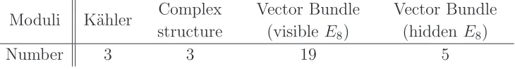
sector bundle will be introduced in the final section. The sheaf cohomologies and their relation to the low-energy spectrum are briefly discussed and the cohomology space of vector bundle moduli is presented. The relevant short and long exact sequences are given in Section 3. The various cohomologies in the intertwined complex of long exact sequences are systematically calculated using two Leray spectral sequences. In Section5 all this information is brought together to compute the number of vector bundle moduli. For the heterotic standard model vacua under consideration, the number of such moduli in the observable sector is found to benobservable = 19.Finally, this formalism is applied

in Section 6 to compute the number of vector bundle moduli in the strongly coupled hidden sector. We find that nhidden = 5. To summarize, the moduli fields are listed in

Table 1.

Moduli K¨ahler Complex structure

Vector Bundle (visible E8)

Vector Bundle (hidden E8)

Number 3 3 19 5

Table 1: Moduli fields in “A Heterotic Standard Model”

2

Preliminaries

In our approach, there are two fundamental ingredients needed to construct a heterotic standard model. The first is a class of Calabi-Yau threefoldsX with fundamental group

Z_3×Z_{3. The second consists of (a moduli space of) stable, holomorphic vector bundles}

V over X with structure group SU(4) which satisfy appropriate physical constraints. Calabi-Yau threefolds of this type were constructed in [28]. Similarly, in [22] the requi-site holomorphic vector bundles were discussed in detail. Here, we simply outline the properties ofX and V that are relevant to this paper.

2.1

The Calabi-Yau Threefold

X

The Calabi-Yau threefold, X, is constructed as follows. Begin by considering a simply connected Calabi-Yau threefold, Xe, which is an elliptic fibration over a dP_{9 surface. It}

was shown in [28] that there are special dP_{9 surfaces which admit a} Z_3×Z_{3 action. A}

suitable fiber product of two such dP_{9 surfaces is then a Calabi-Yau threefold with an}

induced fixed-point freeZ_3×Z_{3 group action. Hence, the quotientX =X/}e ₍Z_{3 ×}Z_{3) is a}

smooth Calabi-Yau threefold that is torus-fibered over a singulardP_{9and has non-trivial}

fundamental group Z_3×Z_{3, as desired.}

Specifically, Xe is a fiber product

e

[image:5.612.124.489.269.318.2]

of two special dP_{9 surfaces B1 andB2. Thus,X}e _{is elliptically fibered over both surfaces}

with the projections

π1 :Xe →B1, π2 :Xe →B2. (2) The surfaces B1 and B2 are themselves elliptically fibered over P1 with maps

β1 :B1 →P1, β2 :B2 →P1. (3)

Together, these projections yield the commutative diagram

dimC= 3 : Xe

π2

? ? ? ? ? ?

π1





 

dimC= 2 : B1

β1 ??

? ? ?

? B2

β2





 

dimC= 1 : P1.

(4)

The invariant homology ring of each special dP_{9 surface is generated by two} Z_{3 ×}Z₃

invariant curve classes f and t with intersections

f2 = 0, f t= 3t2 = 3. (5)

Using projections (2), these can be lifted to divisor classes

τ1 =π−11(t1), τ2 =π2−1(t2), φ =π1−1(f1) =π−21(f2) (6)

onXe satisfying the intersection relations

φ2 =τ₁3 =τ₂3 = 0, φτ1 = 3τ12, φτ2 = 3τ22. (7)

These three classes generate the invariant homology ring of Xe. For example, one can show that X has, generically, six geometric moduli; three K¨ahler moduli and three complex structure moduli.

Finally, the Chern classes of Xe are found to be

c1 TXe

=c3 TXe

= 0, c2 TXe

= 12(τ₁2+τ₂2). (8)

2.2

The Observable Sector Bundle

V

The observable sector bundlesV onXare produced by constructing stable, holomorphic vector bundles Ve with structure group SU(4)⊂E8 over Xe that are equivariant under the action ofZ_3×Z_{3. Then V =V /}e ₍Z_3×Z_{3). One further requires that V and, hence,}

e

The vector bundlesVe are constructed using a generalization of the method of “bundle extensions” [25,27]. Specifically, Ve is the extension1

0−→V2 −→Ve −→V1 −→0 (9)

of two rank two bundles V1 and V2 onXe. These are of the form

Vi =Li⊗π2∗Wi, i= 1,2 (10)

for some line bundlesLi onXe and rank 2 bundlesWi onB2. The rank two bundles Wi

are themselves extensions

0−→ OB2(aif2)−→Wi −→ OB2(bif2)⊗Iki −→0, (11)

whereai, bi are integers and Iki is the ideal sheaf of some ki-tuple of points on B2.

One must specify not only the bundles Ve, but their transformations under Z_{3 ×}Z₃

as well. To do this, first notice that for theZ_3×Z_{3 action on the space of extensions to}

be well-defined, the line bundlesOB2(aif2),OB2(bif2) and Li must be equivariant under

the finite group action. In this case, the space of extensions will carry a representation of Z_3×Z_{3. An invariant class in the extension space defines an equivariant vector}

bundle extension. A rank 4 vector bundle Ve with this property will inherit an explicit equivariant structure from the action ofZ_{3 ×}Z_{3 on its constituent line bundles. Having}

found such aVe, one can construct V =V /e (Z_3×Z_{3) on X.}

As discussed in [20–22], the requirement thatV admit a gauge connection which satis-fies the hermitian Yang-Mills equations and leads to three chiral families of quarks/leptons, no exotic matter and two pairs of Higgs-Higgs conjugate fields (the minimal number) imposes strong constraints on Ve. These are the following. First, in order for the her-mitian Yang-Mills gauge connection to exist on Ve this vector bundle must be (slope) stable. A non-trivial set of necessary conditions for stability are

H0X,e Ve=H0X,e Ve∨

= 0, H0X,e Ve ⊗Ve∨

= 1. (12)

The remaining three physical constraints were shown in [22] to require that

c3 Ve

=−54, h1X,e Ve∨

= 0, h1X,e ∧2Ve= 14 (13)

respectively.

1

The attentive reader will notice that we exchangedV1andV2in the sequence as compared to [20–

A unique (up to continuous moduli) solution forVe that is compatible with all of our constraints2 _{was found in [22]. It is constructed as follows. First consider the rank two} bundles Wi for i= 1,2 on B2. Take W1 to be

W1 =OB2 ⊕ OB2. (14)

Note that this is the trivial extension of (11) with a1 =b1 =k1 = 0. Now let W2 be an equivariant bundle in the space of extension of the form

0−→ OB2(−2f2)−→W2 −→χ2OB2(2f2)⊗I9 −→0, (15)

where for the ideal sheafI9 of 9 points we take a genericZ3×Z3 orbit. Second, choose the two line bundles Li for i= 1,2 on Xe to be

L1 =χ2OXe(−τ1 +τ2) (16)

and

L2 =OXe(τ1−τ2) (17)

respectively. Here, χ1 and χ2 are the two natural one-dimensional representations of

Z_3×Z_{3 defined by}

χ1(g1) =ω , χ1(g2) = 1 ; χ2(g1) = 1, χ2(g2) = ω , (18)

where g1,2 are the generators of the two Z3 factors, χ1,2 are two group characters of

Z_3×Z_{3, and ω=e}2πi3 is a third root of unity.

It follows that the two rank 2 bundles V1,2 defined in eq. (10) are given by

V1 = χ2OXe(−τ1+τ2)⊕χ2OXe(−τ1+τ2)

V2 = OXe(τ1−τ2)⊗π

∗ 2W2.

(19)

The observable sector bundleVe is then an equivariant element of the space of extensions eq. (9).

2.3

Computing the Particle Spectrum

As discussed in detail in [22], the low-energy particle spectrum is given by

ker(D/Ve) =

H0(X,e O_Xe)⊗45

Z3×Z3

⊕H1 X,e ad(Ve)⊗1

Z3×Z3

⊕

⊕H1_{(X,e Ve)⊗16}Z3×Z3 _⊕H1_{(X,e Ve}∨

)⊗16

Z3×Z3

⊕H1_{(X,e ∧}2_Ve)⊗10Z3×Z3 _, (20)

2

where the superscript indicates the invariant subspace under the action of Z_3×Z_3.

The invariant cohomology space (H0_{(X,e O}

e

X)⊗45)

Z3×Z3 corresponds to gauge

super-fields in the low-energy spectrum carrying the adjoint representation of SU(3)C ×

SU(2)L×U(1)Y ×U(1)B−L. The matter cohomology spaces, (H1(X,e Ve)⊗16)

Z3×Z3_,

(H1_{(X,e Ve}∨

)⊗16)Z3×Z3 _{and (H}1_(X,e _∧2_Ve_)⊗10)Z3×Z3 _{were all explicitly computed in [22],}

leading to three chiral families of quarks/leptons (each family with a right-handed neu-trino [55]), no exotic superfields and two vector-like pairs of Higgs-Higgs conjugate superfields respectively. The remaining cohomology space in eq. (20), namely,

H1 _{X,e ad(Ve)⊗1}Z3×Z3_{, (21)}

corresponds to the vector bundle moduli in the low-energy spectrum, see also [8, 47,

48, 56–59]. Since ad(Ve) is a rank 15 vector bundle, its cohomology is much harder to compute than the previous cohomology spaces and, for that reason, was not evaluated in [20–22]. However, vector bundle moduli play an essential role in mu-terms, Yukawa couplings and in the discussion of vacuum stability and the cosmological constant. For these reasons, and to complete the spectrum, this paper will present a formalism for computing eq. (21). We will then use this formalism to explicitly evaluate the number of vector bundle moduli in the heterotic standard model.

3

The Exact Sequences

It is clear from eq. (21) that we must compute the cohomology space H1 _{X,e ad(Ve).} First, recall that the action of the Wilson line on the 1 representation is trivial. Hence, we only need to know the Z_3×Z_{3-invariant part of the cohomology. Second, note that}

ad(Ve) is defined to be the traceless part of Ve⊗Ve∨_{. But the trace part is just the trivial} line bundle, whose first cohomology group vanishes. It follows that the vector bundle moduli are precisely

H1_{X,e ad(Ve)}Z3×Z3 _=H1_{X,e Ve ⊗Ve}∨Z3×Z3

−H1_{X,e O}

e

X

| {z }

=0

Z3×Z3

. (22)

Therefore, the tangent space to the moduli space isH1 _{X,e Ve ⊗Ve}∨Z3×Z3

. To compute this space, one must consider complexes of interlocking exact sequences.

3.1

Short Exact Bundle Sequences

Recall from eq. (9) that the vector bundle Ve is defined by the short exact sequence of bundles

One can tensor this sequence on the right by the bundles V∨

1 , Ve∨ and V2∨ to produce three new short exact sequences which we will refer to as (a), (b) and (c) respectively. Now take the dual of eq. (23). This gives the short exact sequence of bundles

0−→V∨

1 −→Ve ∨

−→V∨

2 −→0, (24)

which we will tensor with vector bundles V2, Ve and V1. Of course, the tensor product is commutative, but we will write it as tensoring on the left. The three resulting short exact sequences will be referred to as (d), (e) and (f) respectively. The six short exact bundle sequences constructed in this manner can be written together as the commutative diagram of exact sequences

(d) (e) (f)

0

0

0

(a) ₀ //_V

2⊗V1∨

/

/_Ve _⊗V∨ 1

/

/_V

1⊗V1∨

/

/₀

(b) ₀ //

V2⊗Ve∨

/

/ _e

V ⊗Ve∨

/

/

V1⊗Ve∨

/

/₀

(c) ₀ //_V

2⊗V2∨

/

/_Ve _⊗V∨ 2

/

/_V

1⊗V2∨

/

/₀

0 0 0

. (25)

3.2

Long Exact Cohomology Sequences

sequences of the form3 ... ... ... ... ...

··· //_Hi−2_(V 1⊗V2∨)

/

/_Hi−1_(V 2⊗V2∨)

/

/_Hi−1_(Ve⊗V∨

2 )

/

/_Hi−1_(V 1⊗V2∨)

/

/_Hi

(V2⊗V2∨)

/

/···

··· //_Hi−1

(V1⊗V1∨)

/

/_Hi

(V2⊗V1∨)

/

/_Hi

(Ve⊗V∨

1 )

/

/_Hi

(V1⊗V1∨)

/

/_Hi+1

(V2⊗V1∨)

/

/···

··· //_Hi−1_(V 1⊗Ve∨)

/

/_Hi

(V2⊗Ve∨)

/

/_Hi

(Ve⊗Ve∨

)

/

/_Hi

(V1⊗Ve∨)

/

/_Hi+1_(V 2⊗Ve∨)

/

/···

··· //_Hi−1_(V 1⊗V2∨)

/

/_Hi

(V2⊗V2∨)

/

/_Hi

(Ve⊗V∨

2 )

/

/_Hi

(V1⊗V2∨)

/

/_Hi+1_(V 2⊗V2∨)

/

/···

··· //_Hi

(V1⊗V1∨)

/

/_Hi+1

(V2⊗V1∨)

/

/_Hi+1

(Ve⊗V∨

1 )

/

/_Hi+1

(V1⊗V1∨)

/

/_Hi+2

(V2⊗V1∨)

/ /··· ... ... ... ... ... _ _ _ _ _ _ _ _ _ _ _ _ _ _ _ _ _ _ _ _ _ _ _ _ _ _ _ _ _ _ _ _ _ _ _ _ _ _ , (26)

where the cohomology spaces in degrees i < 0 or i > 3 vanish for dimension reasons. Note that the object of interest, namely, H1 _{X,e Ve ⊗Ve}∨_{, occurs in this complex. By} evaluating various other cohomology spaces in these sequences, we will be able to ex-plicitly compute H1 _{X,e Ve ⊗Ve}∨_.

3.3

The “Corner” Cohomologies

We begin by noting that the complex is composed of a number of 3×3 blocks, each of the form _ _ _ _ _ _ _ _ _ _ _ _ _ _ _ _ _ _ _ _

C =Hi_V

2⊗V1∨

/

/_Hi_Ve _⊗V∨ 1 / / _ _ _ _ _ _ _ _ _ _ _ _ _ _ _ _ _ _ _ _

Hi_V

1 ⊗V1∨

=A

Hi_V

2⊗Ve∨

/

/_Hi_Ve _⊗Ve∨

/

/_Hi_V

1⊗Ve∨

_ _ _ _ _ _ _ _ _ _ _ _ _ _ _ _ _ _ _ _

D=Hi_V

2⊗V2∨

/

/_Hi_Ve _⊗V∨ 2 / / _ _ _ _ _ _ _ _ _ _ _ _ _ _ _ _ _ _ _ _

Hi_V

1⊗V2∨

=B

, (27)

containing exclusively degree i cohomology spaces. The cohomology spaces at the cor-ners of each block, labeled asA,B,C and D, are particularly amenable to evaluation, so we begin by computing them.

3

Cohomologies A

First consider the cohomology spaces

A=H∗_e

X, V1⊗V1∨

. (28)

It follows from eq. (19) that V1⊗V1∨ is just the rank 4 trivial bundle,

V1⊗V1∨ =OXe

⊕4_{. (29)}

Then, its cohomology spaces are

H∗X, Ve 1⊗V1∨

=H∗(X,e O_Xe)⊕4 (30)

and, therefore,

H0 X, Ve 1⊗V1∨

= 4, H1 X, Ve 1⊗V1∨

= 0,

H2 X, Ve 1⊗V1∨

= 0, H3 X, Ve 1⊗V1∨

= 4, (31)

where we have used the simplifying notation that C⊕4 _{≡ 1}⊕4 _{≡ 4, thought of as a}

Z_3×Z_{3 representation. In fact, throughout this paper we will often denote the trivial}

n-dimensional representation by

1⊕n _{≡n, (32)}

for any positive integer n.

Cohomologies B

Next, we calculate the spaces B given by

H∗X, Ve 1⊗V2∨

. (33)

For notational simplicity, we define

F =V1⊗V2∨. (34)

These cohomology spaces are much harder to compute and will be evaluated using several applications of the Leray spectral sequence. The first Leray sequence is associated with integrating over the elliptic fiber ofπ2 :Xe →B2, hence pushing the cohomology down onto the base surface B2. In this case, one finds4

Hi_{X,e F=} p+q=i

M

p,q

Hp_B

2, Rqπ2∗F

, (35)

4

where the only nonvanishing entries are for p= 0,1,2 (since dimCB₂ = 2) and q= 0,1

(since the fiber ofXe is an elliptic curve). It follows from eq. (19) that

F =O_Xe(−2τ1 + 2τ2)⊕2 ⊗π2∗W2, (36)

where we have used the fact, proven in [22], that W∨

2 = χ22W2. Furthermore, we see from eq. (6) that

O_Xe(τi) =πi∗OBi(ti), i= 1,2. (37)

Combining this with eq. (36) implies

F =hπ∗ 1

OB1(−2t1)

⊗π∗ 2

OB2(2t2)⊗W2

i⊕2

. (38)

Then, using the projection formula and the fact that

Rq_π

2∗

◦π∗ 1 =β

∗

2 ◦ Rqβ1∗

, (39)

which follows from the commutativity of the diagram eq. (4), one finds

Rqπ2∗F =

h

β₂∗Rqβ1∗

OB1(−2t1)

⊗ OB2(2t2)⊗W2

i⊕2

. (40)

Using this expression, we can calculate each cohomology space Hp_(B

2, Rqπ2∗F) in eq. (35), to which we now proceed.

Note that the cohomologies Hp_(B

2, Rqπ2∗F) fill out the 2×3 tableau5

q=1 H0 B₂, R1π_2∗F H1 B₂, R1π_2∗F H2 B₂, R1π_2∗F

q=0 H0 B₂, π_2∗F H1 B₂, π_2∗F H2 B₂, π_2∗F

p=0 p=1 p=2

. (41)

Such tableaux are very useful in keeping track of the elements of Leray spectral se-quences. As is clear from eq. (35), the sum over the diagonals yields the desired coho-mology of F. Let us first evaluate the cohomologies with q = 0. Since the curve −2t1 intersects the fiber ofB1 negatively, that is, −2t1 has negative degree, it follows that

R0β1∗

OB1(−2t1)

=β1∗

OB1(−2t1)

= 0. (42)

Since the push-down vanishes we immediately obtain

Hp_B

2, π2∗F

= 0, p= 0,1,2 (43)

and the Leray tableau eq. (41) becomes

q=1 H0 _B

2,R1π2∗F

H1 _B

2,R1π2∗F

H2 _B

2,R1π2∗F

q=0 _{0 0 0}

p=0 p=1 p=2

. (44)

5

Of course, the zero-th derived push-down is just the ordinary push-down,R0

One must now compute the three cohomologies in the upper row, corresponding to

q= 1. We begin by using the fact that

R1_β

1∗OB1(−2t1) =OP1(−1)

⊕6_{, (45)}

derived in [22]. It follows from this and eq. (40) that

R1π2∗F =

h

β2∗

OP1(−1)⊕6

⊗ OB2(2t2)⊗W2

i⊕2

=

= OB2(2t2−f)⊗W2

⊕12

.

(46)

Using this result, we can now computeHp _B

2, R1π2∗F

by pushing down onto the base

P1 _{of B2 using a second Leray spectral sequence. This is given for each p= 0,1,2 by}

Hp_B

2, R1π2∗F

=

s_M+t=p

s,t

Hs_P1_{, R}t_β

2∗(R1π2∗F)

, (47)

wheres= 0,1 (since dimCP1 = 1) andt = 0,1 (since the fiber ofB2 is one dimensional). From eq. (46) and the projection formula, we find that

Rtβ2∗(R1π2∗F) =

h

OP1(−1)⊗Rtβ_2∗

OB2(2t2)⊗W2

i⊕12

. (48)

Using this expression, one can calculate the cohomology spaces Hs _P1_{, R}t_β

2∗(R1π2∗F)

in eq. (47).

First note that the cohomologiesHs _P1_{, R}t_β

2∗(R1π2∗F)

are determined by the 2×2 Leray tableau

t=1 H0 P1, R1β₂∗(R1π2∗F)

H1 _P1_{, R}1_β

2∗(R1π2∗F)

t=0 H0 P1, β₂∗(R1π2∗F)

H0 _P1_{, β}

2∗(R1π2∗F)

s=0 s=1

. (49)

Let us first evaluate the cohomologies witht= 1. Since 2t2 has positive degree, it follows that

R1β2∗

OB2(2t2)⊗W2

= 0. (50)

Therefore,

HsP1_{, R}1_β2∗(R1_{π2∗F)= 0, s= 0,1 (51)}

and the Leray tableau eq. (49) degenerates to

t=1 0 0

t=0 H0 _P1_,β

2∗(R1π2∗F)

H0 _P1_,β

2∗(R1π2∗F)

s=0 s=1

One must now compute the two cohomologies in the lower row, corresponding to

t= 0. It was shown in [22] that

β2∗

OB2(2t2)⊗W2

=OP1(−2)⊕6⊕ O⊕3

P1 ⊕ OP1(1)⊕3. (53)

Then from eq. (48) one finds that

β2∗

R1π2∗F

=hOP1(−3)⊕2⊕ O_P1(−1)⊕ O_P1

i⊕36

. (54)

Clearly, then

h0P1_{, β2∗(R}1_π2∗F)

= 36. (55)

Using results from [22], we can obtain the corresponding 36-dimensionalZ_3×Z₃

repre-sentation, and conclude that

H0P1_{, β2∗(R}1_π2∗F)=RG⊕4_{, (56)}

whereRG stands for the nine-dimensional “regular representation” ofZ_3×Z_{3 given by}

RG= M 0≤n,m≤2

χn

1χm2 =

= 1⊕χ1⊕χ2⊕χ12⊕χ22⊕χ1χ2 ⊕χ1χ22⊕χ21χ2⊕χ21χ22.

(57)

Applying Serre duality on P1_{, and using the fact that the canonical bundle of} P1 _is

OP1(−2), it follows from eq. (56) that

H1P1_{, β2∗(R}1_π2∗F)=RG⊕16_{. (58)}

These results fill out the remaining entries in the Leray tableau eq. (49) for the push-down onto P1_{. The complete tableau is}

t=1 _{0 0}

t=0 _RG⊕4 _RG⊕16

s=0 s=1

. (59)

Summing the diagonals in eq. (59), we can finally evaluate the q = 1 cohomologies

Hp_(B

2, R1π2∗F) in the first Leray spectral sequence. Recall, that p = 0,1,2 and that

s+t=p. Then

1. p= 0 ⇒ s =t = 0:

H0B2, R1π2∗F

2. p= 1 ⇒ (s = 0, t= 1) or (s= 1, t= 0):

H1B2, R1π2∗F

=RG⊕16_{, (61)}

3. p= 2 ⇒ s =t = 1:

H2B2, R1π2∗F

= 0. (62)

Therefore the complete Leray tableau eq. (41) for the push-down from Xe toB2 is

q=1 _RG⊕4 _RG⊕16 ₀

q=0 _{0 0 0}

p=0 p=1 p=2

. (63)

With this information one can, at last, compute the cohomologies B given in eq. (33). To do this, use the entries in eqns. (63) and (35), recalling thatm =p+q. The results are

H0X, Ve 1⊗V2∨

= 0, H1X, Ve 1⊗V2∨

=RG⊕4,

H2X, Ve 1⊗V2∨

= RG⊕16_{, H}3_{X, Ve}

1⊗V2∨

= 0.

(64)

Cohomologies C

Cohomologies C can be computed directly from the cohomologies B in eq. (64). To do this, one uses Serre duality, the fact that, sinceXe is a Calabi-Yau manifold, its canonical bundle is O_Xe and the property that RG, given in eq. (57), is self-dual. It follows that the Leray tableau for the push-down fromXe to B2 is

q=1 _{0 0 0}

q=0 _{0 RG}⊕16 _RG⊕4

p=0 p=1 p=2

, (65)

and, therefore,

H0X, Ve 2⊗V1∨

= 0, H1X, Ve 2⊗V1∨

= RG⊕16_,

H2X, Ve 2⊗V1∨

= RG⊕4_{, H}3_{X, Ve}

2⊗V1∨

= 0.

(66)

Cohomologies D

Cohomologies Dare evaluated in much the same way as the B cohomologies. However, the calculation is harder and rather unenlightening. For these reasons, we will only state the results. We find that the Leray tableau for the push-down from Xe to B2 is

q=1 ₀ ρ33 1

q=0 ₁ ρ33 0

p=0 p=1 p=2

whereρ33 is a specific 33-dimensional representation of Z3×Z3 given by

ρ33 =RG⊕3⊕χ1⊕χ2⊕χ21⊕χ22⊕χ21χ2⊕χ1χ22. (68)

Therefore,

H0X, Ve 2⊗V2∨

= 1, H1X, Ve 2⊗V2∨

= ρ33,

H2X, Ve 2⊗V2∨

= ρ33, H3

e

X, V2⊗V2∨

= 1.

(69)

4

The Long Exact Sequences

We now systematically proceed to compute the remaining cohomology spaces eq. (26) that will be required to evaluate H1 _{X,e Ve ⊗Ve}∨_{. An important formula that will be} used over and over again in our analysis is the following. Consider an exact sequence

. . .−→ U f1

−→ V −→ W −→ X f2

−→ Y −→ . . . . (70)

Then

dimC(W) = dimC(V) + dimC(X)−rank(f₁)−rank(f₂). (71)

4.1

The

H

0

Cohomologies

We first focus on the 3×3 block of H0 _{cohomologies in eq. (26). Using the “corner} cohomologies” computed in the previous section, the block is

0 0 0 .. .

0 //₀

/

/_H0 _{Ve ⊗V}∨ 1 / /₄

d2 _/

/_RG⊕16

/

/_{· · ·}

0 //_H0 _V

2⊗Ve∨

/

/_H0 _{Ve ⊗Ve}∨

/

/_H0 _V

1⊗Ve∨

/

/_H1 _V

2⊗Ve∨

/

/_{· · ·}

0 //₁

d1

/

/_H0 _{Ve ⊗V}∨ 2 d3 / /₀ /

/ρ₃₃

/

/_{· · ·}

· · · //_RG⊕16

/

/_H1 _{Ve ⊗V}∨ 1 / /₀ /

/_RG⊕4

/ /_{· · ·} ... ... ... ... _ _ _ _ _ _ _ _ _ _ _ _ _ _ _ _ _ _ _ _ _ _ _ _ _ _ _ _ _ _ _ _ _ _ _ _ _ _ _ _ _ _ _ _ _ _ _ _ _ _ , (72)

where we have labeled coboundary maps d1, d2, and d3. The bottom horizontal exact sequence of this box is

0−→1−→H0X,e Ve ⊗V∨ 2

Using formula eq. (71), we find immediately that

H0_{X,e Ve ⊗V}∨ 2

= 1. (74)

Similarly, the right hand vertical exact sequence is

0−→4−→H0X, Ve 1⊗Ve∨

−→0−→0. (75)

It then follows from eq. (71) that

H0X, Ve 1⊗Ve∨

= 4. (76)

It remains to determine H0 _{X,e Ve⊗V}∨ 1

and H0 _{X, Ve} 2⊗Ve∨

to complete theH0 _block, eq. (72). To do that, we need to know the three coboundary mapsd1, d2, andd3. First, consider the top horizontal exact sequence

0−→0−→H0X,e Ve ⊗V∨ 1

−→4 d2

−→RG⊕16_{. (77)}

To evaluateH0 _{X,e Ve ⊗V}∨ 1

, we note that

d2 :H0

e

X,O⊕4

e

X

→H1X, Ve 2⊗V1∨

(78)

is multiplication of constant sections by a choice of extension in Ext1_Xe V1, V2

. For a generic choice of extension, it follows thatd2 is an injective map. This then implies that ker(d2) = 0 and, hence, that rank(d2) = 4. Using this result, eqns. (71) and (77) give

H0X,e Ve ⊗V∨ 1

= 0. (79)

Next, consider the left hand vertical exact sequence

0−→0−→H0X, Ve 2⊗Ve∨

−→1 d1

−→RG⊕16_{. (80)}

An identical proof implies that rank(d1) = 1 and, hence, using eq. (71) we find

H0X, Ve 2⊗Ve∨

= 0. (81)

The last unknownH0_cohomology,H0 _{X,e Ve⊗Ve}∨_{, is contained in the middle vertical} exact sequence given by

0−→0−→H0X,e Ve ⊗Ve∨

−→1 d3

−→H1X,e Ve ⊗V∨ 1

. (82)

It follows from eq. (71) that

H0X,e Ve ⊗Ve∨

Note that rank(d3) can be either 0 or 1. Were rank(d3) = 1, then one would conclude from eq. (83) that H0 _{X,e Ve ⊗Ve}∨ _{vanishes. But this is impossible, because}

H0X,e Ve ⊗Ve∨

=H0X,e O_Xe⊕H0X,e (Ve ⊗Ve∨

)traceless. (84)

Then, using H0 _{X,e O}

e

X

= 1 we see that h0_{(X,e Ve ⊗Ve}∨_{) ≥1. Therefore, rank(d} 3) = 0 and eq. (83) implies

H0X,e Ve ⊗Ve∨

= 1. (85)

In addition to completing the evaluation of the H0 _{cohomologies, eq. (85) is important} since it proves that the vector bundle Ve indeed satisfies the third non-trivial stability condition listed in eq. (12).

4.2

The

H

1

Cohomologies

We now focus on the 3×3 block of H1 _{cohomologies in eq. (26). Since it contains the} space of moduli, H1_{(X,e Ve ⊗Ve}∨_{), this is the final block that we need to consider. The}

H1 _{cohomology block is}

... ... ... ... 0 / /₁ d1 / /₁ / /₀ /

/ρ₃₃

/

/_{· · ·}

· · · //₄

d2

/

/_RG⊕16

/

/_H1 _{Ve ⊗V}∨ 1 / /₀ /

/_RG⊕4

/

/_{· · ·}

· · · //₄

/

/_H1 _V

2⊗Ve∨

/

/_H1 _{Ve ⊗Ve}∨

/

/_H1 _V

1⊗Ve∨

/

/_H2 _V

2⊗Ve∨

/

/_{· · ·}

· · · //₀

/

/ρ₃₃

/

/_H1 _{Ve ⊗V}∨ 2

/

/_RG⊕4

/

/ρ₃₃

/

/_{· · ·}

· · · //₀

/

/_RG⊕4

/

/_H2 _{Ve ⊗V}∨ 1 / /₀ / /₀ / /_{· · ·} .. . ... ... ... ... _ _ _ _ _ _ _ _ _ _ _ _ _ _ _ _ _ _ _ _ _ _ _ _ _ _ _ _ _ _ _ _ _ _ _ _ _ _ _ _ _ _ _ _ _ _ _ _ , (86)

where we have inserted the “corner” cohomologies A, B, C and D as well as the H0 results derived above. We immediately note thatH1 _{X, Ve}

1⊗Ve∨

lies in the right hand vertical sequence

0−→0−→H1X, Ve 1⊗Ve∨

−→RG⊕4 −→0. (87)

It then follows from eq. (71) that

H1X, Ve 1⊗Ve∨

Similarly, one determines that

H1X,e Ve ⊗V∨ 1

=RG⊕16_{−rank(d2)·1 =RG}⊕16_{−4. (89)}

We now proceed to evaluate the remaining elements in the H1 _{block. To do this, it} is essential that one knows the ranks of several coboundary maps in the intertwined sequences. These are hard to determine for the complete cohomology spaces. The problem simplifies, however, if we restrict the complex of sequences to the Z_{3 ×}Z₃

invariant subspace of each cohomology space. Then, using the fact that

RGZ3×Z3

= 1 ρZ3×Z3

33 = 3, (90)

which follow from eqns. (57) and (68) respectively, the H1 _{block and its nearby} coho-mologies simplify to

.. . .. . .. . .. . 0 / /₁ d1 / /₁ d3 / /₀ / /₃ δ1 / /_{· · ·}

· · · //₄

d2 _/

/₁₆ / /₁₂ / /₀ / /₄ / /_{· · ·}

· · · //₄

/

/_H1_(V

2⊗Ve∨)Z3×Z3

/

/_H1_(Ve⊗Ve∨₎Z₃×Z₃

/ /₄ /

/_H2_(V

2⊗Ve∨)Z3×Z3

/

/_{· · ·}

· · · //₀

/ /₃ δ1 /

/_H1_(Ve⊗V∨

2 )

Z₃×Z₃

/ /₄ δ∨ 1 _/ /₃ / /_{· · ·}

· · · //₀

/ /₄ /

/_H2_(Ve⊗V∨

1 )

Z₃×Z₃

/ /₀ / /₀ / /_{· · ·} .. . ... ... ... ... _ _ _ _ _ _ _ _ _ _ _ _ _ _ _ _ _ _ _ _ _ _ _ _ _ _ _ _ _ _ _ _ _ _ _ _ _ _ . (91)

Note that we have indicated two new coboundary maps δ1 and δ1∨ in eq. (91), as well as the maps d1, d2, and d3 introduced previously.

For the invariant cohomology subspaces, one can show

δ1 = 0 (92)

using the cup product in the Leray spectral sequence. We postpone the details to Appendix A. It is exactly at this point that we found it expedient to restrict to the invariant part of the cohomologies. Noting thatδ∨

1 is the Serre dual ofδ1, it follows that

δ∨

as well. To compute the H1 _{cohomologies, we must first know H}2_{(X, Ve}

2 ⊗Ve∨)Z3×Z3. This lies in the vertical sequence

3 δ1

−→4−→H2X, Ve 2⊗Ve∨

Z3×Z3

−→3−→0. (94)

Using eq. (92), we immediately obtain

H2X, Ve 2⊗Ve∨

Z3×Z3

= 7. (95)

Serre duality then implies that

H1X,e Ve ⊗V∨ 2

Z3×Z3

= 7 (96)

as well. Note that this is consistent with the lower horizontal sequence in theH1 _block and eq. (93).

Let us now consider the left hand vertical long exact sequence in theH1 _{block, which} reads in part

1 d1

−→16−→H1X, Ve 2⊗Ve∨

Z3×Z3

−→3 δ1

−→4. (97)

Using eq. (92), the fact, previously established, that rank(d1) = 1 and eq. (71), we find that

H1X, Ve 2⊗Ve∨

Z3×Z3

= 18. (98)

Serre duality then implies

H2X,e Ve ⊗V∨ 2

Z3×Z3

= 18. (99)

Putting this information back into the complex of sequences, we arrive, finally, at ... ... ... ... 0 / /₁ d1 / /₁ d3 / /₀ / /₃ δ1 / /_{· · ·}

· · · //₄

d2 _/

/₁₆ / /₁₂ / /₀ / /₄ / /_{· · ·}

· · · //₄

d4 _//

18

/

/_H1_(Ve⊗Ve∨₎Z3×Z3

/ /₄ δ∨

2 _//

7

/

/_{· · ·}

· · · //₀

/ /₃ δ1 / /₇ δ2 / /₄ δ∨ 1 _/ /₃ / /_{· · ·}

· · · //₀

/ /₄ / /₄ / /₀ / /₀ / /_{· · ·} ... ... ... ... ... _ _ _ _ _ _ _ _ _ _ _ _ _ _ _ _ _ _ _ _ _ _ _ _ _ _ _ _ _ _ _ _ _ _ _ _ . (100)

Note that we have introduced yet more coboundary maps: d4,δ2, andδ∨

5

The Moduli

One can now solve for the tangent space to the moduli space, H1_{(X,e Ve ⊗Ve}∨₎Z3×Z3, of

the observable sector. Of course, the complex dimension of the tangent space equals the number of moduli. To do this, consider the middle horizontal sequence in eq. (100) given by

0−→1−→4 d4

−→18−→H1X,e Ve ⊗Ve∨Z3×Z3

−→4 δ

∨

2

−→7. (101)

One must now determine the rank of the coboundary maps d4 and δ∨2. Since we are restricted to the invariant cohomology subspaces, one can apply methods identical to those used in Appendix A to prove eq. (92). Again, one finds that

δ2∨ = 0. (102)

The rank of d4 can be determined by the exactness of the sequence eq. (101). The beginning of this sequence is

0 φ1

−→1 φ2

−→4 d4

−→18, (103)

where we named the first two maps φ1 and φ2. Exactness implies that im(φ1) = ker(φ2) and, hence, that ker(φ2) = 0. It follows thatφ2 is injective and that im(φ2) = ker(d4) = 1. Therefore, rank(d4) is the difference 4−1 = 3. That is,

rank(d4) = 3. (104)

Then, using eqns. (102), (104), and (71), the exact sequence eq. (101) tells us that the number of moduli of the observable sector vector bundleV =V /e (Z_3×Z_{3) is}

nobservable =h1

e

X,Ve ⊗Ve∨Z3×Z3

= 19. (105)

6

The Hidden Sector Moduli

In the previous section, we computed the number of vector bundle moduli in the ob-servable E8 gauge sector. However, there is also theE8′ hidden sector (in the following, the prime will always denote hidden sector quantities), which potentially contributes moduli fields to the low energy effective action. These moduli interact only gravitation-ally with the fields of the standard model and, therefore, are not immediately relevant. Nevertheless, we would like to compute the hidden sector moduli in this section. The reason is twofold. First, the stability and dynamics of the hidden sector vector bundles is important for the discussion of supersymmetry breaking viaE′

the same formalism as for the observable sector bundles. It serves, therefore, as another, simpler, example of our method. For specificity, we will consider the hidden sector of the strongly coupled heterotic string only. Our formalism is easily applied to the weak coupling case as well.

Recall that in [22], for the case of strong string coupling, we chose the E′

8 hidden sector gauge bundle to be anSU(2) instanton V′

over the Calabi-Yau threefoldX. As usual, we work with the Z_3×Z_{3-equivariant bundleV}e′ _{on the universal covering space}

e

X. The bundle Ve′ _{was explicitly defined by the extension}

0−→V′

2 −→Ve ′

−→V′

1 −→0, (106)

whereV′

1 and V2′ are the line bundles

V′

2 =OXe(2τ1+τ2 −φ), V

′

1 = V2′

∨

=O_Xe(−2τ1−τ2+φ). (107)

Analogous to eq. (25), we find that Ve′_⊗Ve′∨ _{lives in a 3×3 square of short exact} sequences

0

0

0

0 //_ _ _ _ _ _ _ _ _ _ _

_ _ _ _ _ _ _ _ _ _ _

O_Xe(4τ1+ 2τ2−2φ)

/

/_Ve′_⊗V′ 1 ∨

/

/

_ _

_OXe_

/

/₀

0 //_V′

2 ⊗Ve′∨

/

/ _e

V′_⊗Ve′∨

/

/_V′

1 ⊗Ve′∨

/

/₀

0 //_ _

_ _

O_Xe

/

/_Ve′_⊗

V′ 2 ∨

/

/

_ _ _ _ _ _ _ _ _ _ _ _

_ _ _ _ _ _ _ _ _ _ _ _OXe(−4τ1−2τ2+ 2φ)

/

/₀

0 0 0

. (108)

We already computed the “corner cohomologies” in [22]. Here, we simply quote the result that

HpX,e OXe(4τ1+2τ2−2φ)

=H3−p_e

X,OXe(−4τ1−2τ2+2φ)

=

(

RG⊕6 _{p= 1}

Therefore, theH0 _{cohomology block reads} 0 0 0 .. .

0 //₀

/

/_H0 _Ve′_⊗V′ 1 ∨ / /₁ d′

2 _//

RG⊕6

/

/_{· · ·}

0 //_H0 _V′ 2 ⊗Ve′∨

/

/_H0 _Ve′_⊗Ve′∨

/

/_H0 _V′ 1 ⊗Ve′∨

/

/_H1 _V′ 2 ⊗Ve′∨

/

/_{· · ·}

0 //₁

d′

1

/

/_H0 _Ve′_⊗V′ 2 ∨ / /₀ / /₀ / /_{· · ·}

· · · //_RG⊕6

/

/_H1 _Ve′_⊗

V′ 1 ∨ / /₀ / /₀ / /_{· · ·} ... ... ... ... _ _ _ _ _ _ _ _ _ _ _ _ _ _ _ _ _ _ _ _ _ _ _ _ _ _ _ _ _ _ _ _ _ _ _ _ _ _ _ _ _ _ _ _ _ _ _ _ _ _ , (110)

and, using exactly the same reasoning as in Subsection 4.1, we find that d′

1 and d′2 are injective. Exactness of the sequence then implies that

H0X,e Ve′_⊗

V′ 1

∨

=H0X, Ve ′ 2 ⊗Ve

′∨ = 0,

H0X, Ve ′ 1 ⊗Ve

′∨

=H0X,e Ve′ ⊗V′

2 ∨

=H0X,e Ve′

⊗Ve′∨ = 1.

(111)

We proceed to the H1 _{cohomology block, which now becomes} ... ... ... 0 0 0 / /₁ d′ 1 / /₁ / /₀ / /_{· · ·}

0 //₀ //

0 //

1 d′ 2 /

/_RG⊕6

/

/_H1 _Ve′_⊗V′ 1 ∨ / /₀ / /_{· · ·}

0 //₀ //

1 //

1 //

H1 _V′ 2 ⊗Ve

′∨

/

/_H1 _Ve′_{⊗ e}

V′∨

/

/_H1 _V′ 1 ⊗Ve

′∨

/

/_{· · ·}

0 //₁ //

1 //

0 //

0 /

/_H1 _Ve′_⊗

V′ 2 ∨ / /₀ / /_{· · ·} ... ... ... ... ... ... _ _ _ _ _ _ _ _ _ _ _ _ _ _ _ _ _ _ _ _ _ _ _ _ _ _ _ _ _ _ _ _ _ _ _ _ _ _ _ _ _ _ _ _ _ _ _ _ _ _ _ _ _ _ _ _ _ _ _ _ _ _ _ _ , (112)

Since we already determined that d′

1 and d′2 inject, and therefore

coker(d′₁) = coker(d′₂) = RG⊕6−1, (113)

we can directly read off that

H1X,e Ve′_⊗

V′ 1

∨

=H1X, Ve ′ 2 ⊗Ve

′∨

=RG⊕6_−1,

H1X, Ve ′ 1 ⊗Ve

′∨

=H1X,e Ve′ ⊗V′

2 ∨

= 0

from the long exact sequences eq. (112). Finally, the middle horizontal long exact sequence

0−→0−→1−→∼ 1−→0 RG⊕6₋₁ ∼

−→H1 X,e Ve′

⊗Ve′∨

−→0−→ · · · (115)

yields

H1X,e Ve′_{⊗ e}

V′∨

=RG⊕6 _{−1. (116)}

Hence, the number of vector bundle moduli of V′ _=Ve′_/(Z

3×Z3) is the invariant part of eq. (116). Using eq. (90)), we find that

nhidden =h1

e

X,Ve′

⊗Ve′∨Z3×Z3

= 6−1 = 5. (117)

We conclude that there are 5 vector bundle moduli in the hidden sector of the strongly coupled string.

Acknowledgments

We are grateful to B. Nelson for enlightening discussions. This research was supported in part by the Department of Physics and the Math/Physics Research Group at the University of Pennsylvania under cooperative research agreement DE-FG02-95ER40893 with the U. S. Department of Energy and an NSF Focused Research Grant DMS0139799 for “The Geometry of Superstrings.” T. P. is partially supported by an NSF grant DMS 0403884.

Appendix A

The Coboundary Map

δ

1

The purpose of this Appendix is to determine the coboundary map

δ1 :H1

e

X, V2⊗V2∨

Z3×Z3

→H2X, Ve 2⊗V1∨

Z3×Z3

(118)

associated with the short exact sequence of equivariant vector bundles (see eq. (24))

0−→V2⊗V1∨ −→V2⊗Ve∨ −→V2⊗V2∨ −→0. (119) The choice of extension V2⊗Ve∨ is precisely the choice of an element xof the Ext-space

x∈Ext1_XeV2⊗V2∨, V2⊗V1∨

Z3×Z3

=H1X, Ve 2⊗V1∨

Z3×Z3

. (120)

Therefore, x must determine the coboundary map δ1. One finds that it is the cup product, that is, the usual wedge product combined with a suitable contraction of vector bundle indices,

δ1 :H1

e

X, V2⊗V2∨

Z3×Z3

→H2X, Ve 2⊗V1∨

Z3×Z3

Note that the cohomology degree is additive. Since x is a degree 1 cohomology class, the image of δ1 is indeed of degree 2. Nevertheless, we claim that the product map

∧:H1X, Ve 2⊗V2∨

Z3×Z3

| {z }

∋ v

⊗H1X, Ve 2⊗V1∨

Z3×Z3

| {z }

∋ x

→H2X, Ve 2⊗V1∨

Z3×Z3

| {z }

∋ δ1(v)=v∧x

(122)

vanishes because of a refined degree stemming from the elliptic fibration. This can be seen as follows. Let us determine the cohomology spaces using the Leray spectral sequences eqns. (65) and (67) corresponding to the π2 :Xe → B2 fibration. First, note that the cohomology always comes from the π2∗ push-down, and not the R1π2∗ part:

H1X, Ve 2⊗V2∨

=ρ33 ⇐

q=1 ₀ ρ33 1

q=0 ₁ ρ33 0

p=0 p=1 p=2

H1X, Ve 2⊗V1∨

=RG⊕16 ⇐

q=1 _{0 0 0}

q=0 _{0 RG}⊕16 _RG⊕4

p=0 p=1 p=2

H2X, Ve 2⊗V1∨

=RG⊕4 ⇐

q=1 _{0 0 0}

q=0 _{0 RG}⊕16 _RG⊕4

p=0 p=1 p=2

, (123)

where we marked the relevant entry in the corresponding tableau in bold face. Hence, the product map, eq. (122), simplifies to

∧:H1X, πe 2∗ V2⊗V2∨

Z3×Z3

⊗H1X, πe 2∗ V2⊗V1∨

Z3×Z3

→

→H2X, πe 2∗ V2 ⊗V1∨

Z3×Z3

. (124)

These cohomology spaces are, in turn, determined by the Leray spectral sequence cor-responding to the β2 :B2 →P1 fibration:

H1X, πe 2∗ V2⊗V2∨

= ρ33 ⇐

t=1 _RG⊕3 ₀

t=0 ₁ (χ1+χ₁2)(1+χ2+χ2₂)

s=0 s=1

H1X, πe 2∗ V2⊗V1∨

= RG⊕16 _⇐

t=1 _RG⊕16 _RG⊕4

t=0 0 0

s=0 s=1

H2X, πe 2∗ V2⊗V1∨

= RG⊕4 _⇐

t=1 _RG⊕16 _RG⊕4

t=0 _{0 0}

s=0 s=1

where we notice that only theR1_β

2∗ push-down contributes to the invariant part of the cohomology spaces. Hence, the product map, eq. (124), simplifies once more to

∧:H0_{X, Re} 1_β

2∗π2∗ V2⊗V2∨

Z3×Z3

⊗H0_{X, Re} 1_β

2∗π2∗ V2⊗V1∨

Z3×Z3

→

→H1X, Re 1β2∗π2∗ V2 ⊗V1∨

Z3×Z3

. (126)

But this product is now zero for degree reasons: the product of two degree 0 cohomol-ogy spaces is again of degree 0, and not 1. Therefore, the product map specified in eqns. (126), (124), and (122) is the zero map. That is,

δ1 = 0, (127)

as claimed.

Bibliography

[1] D. J. Gross, J. A. Harvey, E. J. Martinec, and R. Rohm, Heterotic string theory. 2. the interacting heterotic string, Nucl. Phys. B267(1986) 75. 1

[2] A. Sen, The heterotic string in arbitrary background field, Phys. Rev.D32 (1985) 2102. 1

[3] M. Evans and B. A. Ovrut, Splitting the superstring vacuum degeneracy,Phys. Lett. B174(1986) 63. 1

[4] J. D. Breit, B. A. Ovrut, and G. C. Segre, E6 symmetry breaking in the

superstring theory, Phys. Lett. B158(1985) 33. 1

[5] P. Candelas, G. T. Horowitz, A. Strominger, and E. Witten, Vacuum configurations for superstrings, Nucl. Phys.B258 (1985) 46–74. 1

[6] P. Candelas, G. T. Horowitz, A. Strominger, and E. Witten, Superstring phenomenology, . Presented at Symp. for Anomalies, Geometry and Topology, Argonne, IL, Mar 28-30, 1985 and at 4th Marcel Grossmann Conf. on General Relativity, Rome, Italy, Jun 17-21, 1985. 1

[7] P. S. Aspinwall, B. R. Greene, K. H. Kirklin, and P. J. Miron, Searching for three generation Calabi-Yau manifolds,Nucl. Phys. B294(1987) 193. 1

[9] B. R. Greene, K. H. Kirklin, P. J. Miron, and G. G. Ross, 27**3 yukawa couplings for a three generation superstring model, Phys. Lett. B192(1987) 111. 1

[10] G. Curio, Chiral matter and transitions in heterotic string models,Phys. Lett.

B435(1998) 39–48, [hep-th/9803224]. 1

[11] B. Andreas, G. Curio, and A. Klemm, Towards the Standard Model spectrum from elliptic Calabi- Yau, Int. J. Mod. Phys. A19 (2004) 1987, [hep-th/9903052]. 1

[12] R. Donagi, A. Lukas, B. A. Ovrut, and D. Waldram,Holomorphic vector bundles and non-perturbative vacua in M-theory, JHEP 06 (1999) 034, [hep-th/9901009]. 1

[13] A. Krause, A small cosmological constant, grand unification and warped geometry,

hep-th/0006226. 1

[14] B. Andreas, S.-T. Yau, G. Curio, and D. H. Ruip´erez, Fibrewise T-duality for D-branes on elliptic Calabi-Yau, J. High Energy Phys. (2001), no. 3 Paper 20, 13. 1

[15] B. Andreas, G. Curio, and R. Minasian,Anomalous d-brane charge in f-theory compactifications, JHEP09 (2000) 022, [hep-th/0007212]. 1

[16] B. Andreas and D. Hernandez-Ruiperez, Comments on N = 1heterotic string vacua, Adv. Theor. Math. Phys. 7(2004) 751–786, [hep-th/0305123]. 1

[17] G. Curio and A. Krause, Enlarging the parameter space of heterotic M-theory flux compactifications to phenomenological viability,Nucl. Phys.B693 (2004) 195–222, [hep-th/0308202]. 1

[18] G. Curio, Standard Model bundles of the heterotic string,hep-th/0412182. 1

[19] R. Blumenhagen, G. Honecker, and T. Weigand,Loop-corrected compactifications of the heterotic string with line bundles,hep-th/0504232. 1

[20] V. Braun, Y.-H. He, B. A. Ovrut, and T. Pantev, A heterotic Standard Model,

Phys. Lett. B618 (2005) 252–258, [hep-th/0501070]. 1,2.2,1, 2.3

[21] V. Braun, Y.-H. He, B. A. Ovrut, and T. Pantev, A Standard Model from the

E8×E8 heterotic superstring, JHEP 06 (2005) 039, [hep-th/0502155]. 1,2.2, 1, 2.3

[23] R. Donagi, B. A. Ovrut, T. Pantev, and D. Waldram, Standard-Model bundles on non-simply connected Calabi-Yau threefolds, JHEP 08 (2001) 053,

[hep-th/0008008]. 1

[24] R. Donagi, B. A. Ovrut, T. Pantev, and D. Waldram, Standard-Model bundles,

Adv.Theor.Math.Phys. 5 (2002) 563–615, [math.AG/0008010]. 1

[25] R. Donagi, B. A. Ovrut, T. Pantev, and D. Waldram, Spectral involutions on rational elliptic surfaces,Adv.Theor.Math.Phys. 5 (2002) 499–561,

[math.AG/0008011]. 1, 2.2

[26] B. A. Ovrut, T. Pantev, and R. Reinbacher, Invariant homology on Standard Model manifolds, JHEP 01 (2004) 059, [hep-th/0303020]. 1

[27] R. Donagi, B. A. Ovrut, T. Pantev, and R. Reinbacher, SU(4)instantons on Calabi-Yau threefolds with Z_2×Z_{2 fundamental group, JHEP 01 (2004) 022,}

[hep-th/0307273]. 1, 2.2, 2

[28] V. Braun, B. A. Ovrut, T. Pantev, and R. Reinbacher, Elliptic Calabi-Yau threefolds with Z3×Z3 wilson lines, JHEP 12(2004) 062, [hep-th/0410055]. 1, 2,2.1

[29] R. Donagi, Principal bundles on elliptic fibrations, Asian J. Math 1 (1997) no. 2 214–223, [alg-geom/9702002]. 1

[30] R. Friedman, J. Morgan, and E. Witten, Vector bundles and F theory, Commun. Math. Phys. 187 (1997) 679–743, [hep-th/9701162]. 1

[31] R. Friedman, J. Morgan, and E. Witten, Principal G-bundles over elliptic curves,

Math.Res.Lett. 5 (1998) 97–118, [alg-geom/9707004]. 1

[32] R. Friedman, J. Morgan, and E. Witten, Vector bundles over elliptic fibrations,

alg-geom/9709029. 1

[33] D.-E. Diaconescu and G. Ionesei, Spectral covers, charged matter and bundle cohomology,JHEP 12 (1998) 001, [hep-th/9811129]. 1

[34] R. Donagi, Y.-H. He, B. A. Ovrut, and R. Reinbacher, Moduli dependent spectra of heterotic compactifications,Phys. Lett. B598 (2004) 279–284,

[hep-th/0403291]. 1

[36] B. A. Ovrut, T. Pantev, and R. Reinbacher, Torus-fibered Calabi-Yau threefolds with non-trivial fundamental group, JHEP 05 (2003) 040, [hep-th/0212221]. 1

[37] R. Donagi, Y.-H. He, B. A. Ovrut, and R. Reinbacher, Higgs doublets, split multiplets and heterotic SU(3)C ×SU(2)L×U(1)Y spectra, Phys. Lett. B618

(2005) 259–264, [hep-th/0409291]. 1

[38] R. Donagi, Y.-H. He, B. A. Ovrut, and R. Reinbacher, The spectra of heterotic Standard Model vacua, JHEP 06 (2005) 070, [hep-th/0411156]. 1

[39] E. I. Buchbinder and B. A. Ovrut,Vacuum stability in heterotic M-theory,Phys. Rev. D69 (2004) 086010, [hep-th/0310112]. 1

[40] E. I. Buchbinder, B. A. Ovrut, and R. Reinbacher, Instanton moduli in string theory,JHEP 04 (2005) 008, [hep-th/0410200]. 1

[41] B. A. Ovrut, T. Pantev, and J. Park, Small instanton transitions in heterotic M-theory,JHEP 05 (2000) 045, [hep-th/0001133]. 1

[42] E. Buchbinder, R. Donagi, and B. A. Ovrut, Vector bundle moduli and small instanton transitions, JHEP06 (2002) 054, [hep-th/0202084]. 1

[43] E. I. Buchbinder, R. Donagi, and B. A. Ovrut, Superpotentials for vector bundle moduli,Nucl. Phys. B653(2003) 400–420, [hep-th/0205190]. 1

[44] E. I. Buchbinder, R. Donagi, and B. A. Ovrut, Vector bundle moduli

superpotentials in heterotic superstrings and M-theory, JHEP 07 (2002) 066, [hep-th/0206203]. 1

[45] Y.-H. He, B. A. Ovrut, and R. Reinbacher, The moduli of reducible vector bundles, JHEP03 (2004) 043, [hep-th/0306121]. 1

[46] G. Curio and A. Krause, G-fluxes and non-perturbative stabilisation of heterotic M-theory,Nucl. Phys. B643(2002) 131–156, [hep-th/0108220]. 1

[47] K. Becker and L.-S. Tseng, Heterotic flux compactifications and their moduli,

hep-th/0509131. 1, 2.3

[48] B. de Carlos, S. Gurrieri, A. Lukas, and A. Micu,Moduli stabilisation in heterotic string compactifications, hep-th/0507173. 1, 2.3

[49] E. I. Buchbinder, Five-brane dynamics and inflation in heterotic M-theory,Nucl. Phys. B711(2005) 314–344, [hep-th/0411062]. 1

[51] M. Becker, G. Curio, and A. Krause, De Sitter vacua from heterotic M-theory,

Nucl. Phys.B693 (2004) 223–260, [hep-th/0403027]. 1

[52] E. I. Buchbinder, On open membranes, cosmic strings and moduli stabilization,

hep-th/0507164. 1

[53] A. Borisov, E. I. Buchbinder, and B. A. Ovrut, The dynamics of small instanton phase transitions, hep-th/0508190. 1

[54] K. Becker, M. Becker, and A. Krause, M-theory inflation from multi M5-brane dynamics, Nucl. Phys.B715 (2005) 349–371, [hep-th/0501130]. 1

[55] J. Giedt, G. L. Kane, P. Langacker, and B. D. Nelson, Massive neutrinos and (heterotic) string theory, hep-th/0502032. 2.3

[56] J. Distler, B. R. Greene, K. H. Kirklin, and P. J. Miron, Calculating endomorphism valued cohomology: Singlet spectrum in superstring models,

Commun. Math. Phys. 122 (1989) 117–124. 2.3

[57] R. Blumenhagen, Target space duality for (0,2) compactifications, Nucl. Phys.

B513(1998) 573–590, [hep-th/9707198]. 2.3

[58] G. Curio and R. Y. Donagi, Moduli in N = 1heterotic/F-theory duality, Nucl. Phys. B518(1998) 603–631, [hep-th/9801057]. 2.3

[59] G. Lopes Cardoso, D. Lust, and T. Mohaupt, Moduli spaces and target space duality symmetries in (0,2) Z_{N orbifold theories with continuous Wilson lines,}