Towards virtual testing of compression systems in gas turbine engines

City, University of London Institutional Repository

Citation

:

This is the accepted version of the paper.

This version of the publication may differ from the final published

version.

Permanent repository link:

Link to published version

:

Copyright and reuse:

City Research Online aims to make research

outputs of City, University of London available to a wider audience.

Copyright and Moral Rights remain with the author(s) and/or copyright

holders. URLs from City Research Online may be freely distributed and

linked to.

NAFEMS International Journal of CFD Case Studies, 9, March 2011

Towards virtual testing of compression systems in gas turbine

engines

A. I. Sayma

University of Sussex

Thermo-Fluid Mechanics Research Centre School of Engineering and Design

Brighton BN1 9QT, UK

Abstract

Current trends in the computational fluid dynamics (CFD) analysis of gas turbine engines are in the direction of the so called “virtual testing”. Although this term is used nowadays loosely in the context of this application, the ultimate objective of virtual tests is to replace partly or fully rig and engine tests during the design and certification of engines. In the past few decades, significant developments have been achieved in the discretisation methods and the associated CFD algorithms. Combined with the rapid developments in hardware in both speed and memory which are becoming increasingly available at affordable prices, the simulation of full engine or rig tests are increasingly becoming a reality.

This paper describes a method by which virtual tests can be conducted on a low pressure compression system of a gas turbine engine using smart boundary conditions and allowing the sweep along a speed characteristic or sweep along a working line during the mapping of the compressor characteristic in a similar fashion to a typical rig test. The low pressure compression system is equipped with a variable downstream nozzle and the rotational speed is allowed to vary during the computations. The simulations are validated using NASA rotor 67 experimental data against which good agreement was obtained.

Keywords: Low pressure compression system, turbofan engines, boundary conditions, outflow guide vanes, steady-state analysis, virtual testing, NASA rotor 67

Abbreviations

LPC: Low Pressure Compression system OGV: Outflow Guide Vanes

CGV: Core Guide Vane

CFD: Computational Fluid Dynamics

1. Introduction

unsteadiness resulting either from interactions of stationary and rotating components or the change of rotational speed or both. In addition, distortions due to non-uniform inlet or exit conditions or component damage such as those resulting from bird strikes, ice damage or any other foreign object or loose component damage, may give rise to a number of flow problems resulting in subsequent mechanical problems.

These complex problems mostly require large-scale numerical models with multi-blade row and multi-passage incorporating all necessary engineering features as accurately as possible and in a unified fashion to enable accurate simulation. An approach which is being increasingly called “virtual testing”. Such an approach is justified, if not dictated, by available evidence from a wide body of literature (see for example Wu et al. 2004 and 2005, Vahdati et al 2007, Sayma et al. 2007) in the simulation of turbomachinery in the past few years. For instance, realistic core compressor modelling requires the consideration of all blade-rows, not only because of strong interactions between these, but also due to rotating stall, acoustic resonance and surge for which the entire compressor volume may need to be taken into account (Vahdati et al. 2007, Wu et al. 2005). Similarly, both the forced response and the flutter behaviour of fan assemblies are greatly influenced by the entire low-pressure compression domain consisting of the flight intake and its droop, fan assembly, outflow guide vanes and the pylon (Sayma et al. 2007). From an industrial perspective, the development and validation of such a methodology will allow the evaluation of engine designs on “virtual test rigs” using large-scale numerical models, thus reducing costs significantly by decreasing the number of development engine builds and physical rig tests.

Recent years have witnessed significant progress in the development of numerical procedures for the solution of the flow equations. This combined with the rapid progress in the availability of cheap computing power, makes the use of virtual tests in the design cycle a realistic approach. A prediction tool should possess the following features (a) a fast, accurate and robust flow solver; (b) an efficient spatial discretisation with optimum meshing capability of complicated flow domains, and (c) a convenient and accurate way of prescribing flow boundary conditions. In the past two decades, significant progress has been made towards the fulfilment of the first two requirements. For instance, structured grids are beginning to be superseded by unstructured grids of mixed elements, particularly when complex geometric features need to be accounted for such as fillet radii, bleed holes and variable guide vane pins. Indeed, structured grids are easy to generate for blade geometries but can be of poor quality with local regions of inappropriate refinement in complex geometries. They are also difficult to use with multi-component geometries. On the other hand, semi-structured grids (Sbardella et al 1999) provide an optimum way of discretising blade geometries and can be combined with unstructured grids to provide an efficient method of discretising complex multi-component turbomachinery domains.

operating point to establish the boundary conditions that should be imposed. In these cases, intensive user interference required to perform these simulations. While it is possible to script the process to overcome this problem, a more systematic approach is proposed here. To allow a virtual test to mimic an actual engine or rig test, the simulation system must allow the following:

• A method of prescribing boundary conditions consistent with the variation of

rotational speed and variations of the downstream throttle is varied. These are typically the main variables during an actual test.

• A system that allows for the variation of the rotational speed and automatic

changes of the throttle during the simulation.

• Variation of the blade geometry as the speed and throttle change. The speed

changes produce changes in the blade shape due to the so called centrifugal untwist of the blades. The variation of the speed and throttle cause a further aerodynamic untwist which is a function of the flow conditions (Wilson, 2007)

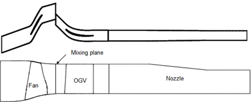
A useful method for prescribing boundary conditions for turbomachinery fans was proposed by Vahdati et al. (2005). In this method, the fan domain is extended upstream where ambient conditions can be applied at inlet. At the outflow, the domain is extended and a choked nozzle is added. This allows for simulations to be conducted along the speed characteristic by changing the nozzle size at different points on the speed characteristic without having to change the boundary conditions (see Figure 1). It is claimed that this method allows for the simulations to approach the stall boundary closer than standard back pressure boundary conditions allow. This method was used by Wu et al. (2004) to map the entire fan characteristic. The simulations were subsequently used for aero acoustic computations of the fan and intake duct.

This work was extended by Sayma (2007) to the full Low Pressure Compression System (LPC) of a turbofan engine which includes the fan, intake duct, and flow split between the core and bypass. The solution domain included two guide vanes downstream that remove the swirl from the flow. One is in the core and the other in the bypass. Both guide vanes were followed by variable area nozzles. Both nozzles are varied at the start of the analysis until the intended split of the flow is obtained between the core and the bypass at the working line. Consequently, and in a manner similar to an actual rig test, the core nozzle is kept fixed, while the bypass nozzle is varied from point to point to map the speed characteristic.

Whole Intermediate Pressure (IP) compressor simulations for a three-spool engine were reported by Wu et al. (2005). These simulations focused on both compressor performance and forced response of rotor blades. The results were validated mainly against other computational data.

calculate the blade deformation. These are then used to deform the aerodynamic mesh to follow the structural deformations. In principle, this approach can be used during a variable speed simulation by retaining the mode shapes and centrifugal untwist of the blade at discrete points along the engine working line. These can then be used throughout a variable speed calculation and interpolation between those points can be performed if intermediate speeds are required. Ultimately, if a non-linear structural model is integrated with the flow solver, the blade shape can be obtained directly as the speed and aerodynamic loads are changed.

This paper will focus on the second bullet point above by extending the work of Vahdati et al. and Sayma above by both allowing simulations as the speed is varied and a complete speed characteristic map in a single run. The characteristic map of NASA rotor 67 blades is mapped at various speeds and the results are compared with the experimental data available at the design speed. Steady state point simulations as the speed or throttle are changed are performed using a single blade passage of the fan. An outflow guide vane is added to remove the swirl downstream, and a variable area nozzle is then added downstream of the vane. Both rotational speed and nozzle area could be varied during the computation. Although the analysis is done for the steady state characteristic, this principle is applicable for whole annulus unsteady computations. Most previous work was validated against other computational data or very limited proprietary engine or rig data. This paper will validate the computations against well documented public domain detailed experimental data.

Two other related issues are addressed in this paper. The first is the difference between the fan characteristic observed by Sayma (2007) between the downstream nozzle approach and the standard backpressure variation approach. The second is the importance of introducing a swirl removal guide vane before the nozzle is added.

The next section will describe the underlying numerical model and the methodology used to prescribe boundary conditions and vary the speed. Section 3 will describe the results for NASA rotor 67 and comparison with experimental data. Section 4 will focus on the issues mentioned in the previous paragraph and lessons learned. This will be followed by concluding remarks.

2. The Numerical model

2.1 Description of the flow solver

This subsection will describe the underlying flow solver and meshing methodology used throughout this work.

The meshing methodology uses a mixture of unstructured and semi-structured grids as appropriate to the component at hand. Hence the flow solver must be able to handle unstructured grids of mixed elements such as tetrahedra, pentahedra, hexahedra and wedges. The code used in this study (SURF) is based on the methodology developed by Sayma et al. 2000. The aerodynamic part of the code is an edge-based solver for the Reynolds-averaged compressible Navier-Stokes equations and both Spallart-Allmaras and the standard k−εturbulence models are implemented. Near the solid

equations up to the wall and then by using the wall damping terms of the turbulence models (Spalart and Allmaras 1994). Another alternative, which allows substantial savings in computational time, is the use of slip conditions with a wall shear stress which is calculated via standard wall functions. The second approach was used in this work for computational efficiency.

The central differencing scheme used in the code is stabilised using a mixture of second- and fourth-order matrix artificial dissipation. In addition, a pressure switch, which guarantees that the scheme is total variation diminishing (TVD) and reverts back to a first-order Roe scheme in the vicinity of discontinuities, is used for numerical robustness. The resulting semi-discrete system of equations is advanced in time using a point-implicit scheme with Jacobi iterations and dual time stepping. Such an approach allows relatively large time steps for the external Newton iterations. Solution acceleration techniques, such as residual smoothing and local time stepping, are employed for steady-state flow calculations. For unsteady flow computations, an outer Newton iteration procedure is used where the time steps are dictated by the physical constraints of capturing the phenomena of interest and fixed throughout the solution domain. Within the Newton iteration, the solution is advanced to convergence using the traditional acceleration techniques associated with steady-state flow solutions.

An important additional feature is allowing for the rotational speed to vary during the computation. As the rotational speed is varied, the grid points at the surface are moved to take a new blade shape due to the change in centrifugal load. This blade shape is stored at discrete points along the fan speed and values are interpolated if intermediate speeds are required. The mesh is modified using mesh movement technique. This is designed to ensure that the near wall grid moves solidly with the blade to keep near wall resolution, while the movement is absorbed in the coarser grid far from the wall. At each discrete point, the solution is allowed to converge and once prescribed convergence criteria are reached, the analysis moves to the next point along the working line. The code also allows tracing the speed characteristic from choke to stall by varying the throttle. The throttle is varied by moving the grid points in the nozzle to either reduce or increase its area. The combination of rotational speed and throttle variations allow to calculate a complete compressor characteristic map in a single calculation.

2.2 The domain and smart boundary conditions

outflow guide vane (OGV) geometry from the test rig was not available, so an OGV was designed for the purpose of this work. All components are solved in their respective inertial frame. Thus at the interface between rotating components and stationary components, mixing planes are used for steady state computations and sliding planes are used for unsteady computations. For mixing planes, circumferentially mass averaged boundary conditions are interchanged between blade rows. For sliding planes, local boundary conditions are interpolated from for each point on the sliding plane from the opposing boundary face nodes.

For a turbofan engine low pressure compression (LPC) system (which includes, the intake duct, fan, downstream guide vanes and bypass duct), the method is based on the modelling of the whole LPC domain which includes the intake duct, the fan assembly, the OGVs and the Core Guide Vanes (CGVs) (Fig 2). Further components, such as the pylon, can be added if required. The flow domain is extended upstream to enable the imposition of ambient conditions and the natural build up of the intake and spinner boundary layers. Two variable nozzles are used downstream, one controlling the core flow and the other the bypass flow, and ambient conditions are used downstream of both nozzles. The core/bypass flow split and the downstream pressure are controlled by varying both nozzles. The region between the fan assembly and the downstream components, including the splitter, is represented using an unstructured grid which is joined to the semi-structured blade grid. Semi-unstructured grids are generated using paved triangular grids in the blade-to-blade direction that are connected in a structural manner in the radial direction. For steady-state flow analysis mixing planes are used between the blade rows, allowing a single passage representation to be used. One of the distinct advantages of this method is that it allows accommodating different designs of a given component, say the OGV, with minimum effort without having to re-mesh the rest of the domain. It should be noted that a grid independence study was performed and the grids used were deemed suitable for the purpose of the concepts introduced in this paper.

In order to predict the pressure distribution and the flow split downstream, the model requires only two parameters, namely the fan rotational speed and the bypass ratio at the working line. Such quantities are usually known from rig tests or from the design intent during the design process through the engine performance model. Once a working line operating point is known in terms of a given pressure ratio, mass flow and mass split, the corresponding speed characteristic can be mapped by fixing the core nozzle and varying the bypass nozzle, a procedure which mimics an LPC rig test procedure (Sayma 2007)

3.

NASA rotor 67 Characteristic

The grid used in this study was shown in Fig. 3. The fan domain contains about 500,000 grid points. The tip gap was assumed to be constant at 2% of the span. As mentioned in section 2, the stator blade geometry from the rig was not available for this study, so an OGV was specifically designed with the only objective of removing the swirl from the flow as it enters the variable area nozzle. The OGV grid contained about 350,000 nodes. A variable area nozzle was added at the back of the OGV. The three components were treated as separate grids joined together in a single mesh with mixing planes at the interface boundary. Although in principle, the OGV and the nozzles could have been treated as a single mesh, the present set up allows for freely changing individual components while keeping the others allowing for faster mapping of the characteristic, or modifying the design of one component while keeping the other components the same.

Two types of analyses were performed. The first is a speed characteristic sweep. In this analysis, a probing investigation is done first to find out the choke or the stall boundary. In this analysis, the choke boundary was located. This requires about 3, or 4 steady-state runs each with a single nozzle. Once the nozzle corresponding to the choke boundary is found, this grid is used to start the analysis. The speed characteristic is traced by a series of step changes in the nozzle size during the analysis. Each time the nozzle is changed, it is kept fixed until the convergence criteria are met. Convergence criteria are user defined and can be residuals, or integrated inlet or blade surface quantities such as mass flow rate and lift. The convergence criteria can be based on either the residuals from the flow equations or the mass flow rate or both. Once the solution is converged, the nozzle area is reduced again. The stall boundary is located if the solution does not converge after a pre-specified number of iterations. As the stall boundary is approached, the nozzle size changes are reduced to allow a smooth approach to stall. The analysis was performed at four different speeds: design speed (which will be referred to as 100% speed), 90% speed 80% speed and 60% speed. The same fan geometry was used for all speeds and thus, the changing fan shape at different speeds was not taken into account as a structural model was not available for this fan. This should not have an influence on the main objectives of this exercise. However, in principle, taking this into account is straight forward as mentioned earlier.

Figure 4 shows a typical convergence time history plot. It shows that each time the nozzle size is changed; the residuals jump up and about 3000 time steps are needed for convergence after that. In this run the convergence criteria was switched off and 3000 time steps were used per nozzle change. It can be seen how convergence deteriorates as the stall boundary is reached. The last two points were discarded in the reported fan characteristic below. The full sweep takes approximately 24 hours on two quad-core processors of a 3GHz Intel cluster. It should be noted that the CPU time can be reduced significantly be making larger step changes in the nozzle size near choke at the vertical side of the characteristic.

reported in the experimental results. This is thought to be due to the short inlet used in this study which does not allow for enough build up of wall boundary layer as the flow approaches the tip. Figure 6 shows a comparison of the adiabatic efficiency with the experimental results where the agreement is also excellent. Mach number contours in the blade-to-blade direction at 90% span (measured from hub) are shown for three points, near choke, at peak efficiency and near stall in Fig 7. These are in good agreement with those reported by Chima (1991) in terms of the shock position and maximum Mach number. They also show qualitatively typical fan behaviour with the shock moving from the back of the passage at choke to near the leading edge at peak efficiency and expelled near stall. Figure 8 shows the pressure contours at the pressure and suction side of the blade at the point of peak efficiency, which also compares very well with the experimental results presented by Chima (1991).

Circumferentially averaged profiles for the total pressure rise, total temperature rise and fan outlet flow angle are shown in Figs 9, 10 and 11 respectively, compared with measured data. The total temperature rise and flow angle are in good agreement with measurements. This is expected for the flow angle in particular where the flow angle is expected to follow closely the blade exit angle as long as there is no significant flow separation. However, the lower half of the pressure rise seems to be over predicted. This is also evident to a less extent in the temperature rise profile. This might have been affected by the shape of the hub section profile ahead of the fan where the spinner was replaced in this geometry by a more gently varying boundary. This was not investigated further in this study as it is not a main part of the objectives here.

The second type of analysis in this study was performed by sweeping along a working line by keeping the nozzle size fixed and changing the speed of the fan in discrete steps. For each step, the solution was converged and the speed was changed once the abovementioned convergence criteria are met. The speed was traced from 60% to over 100%. Figure 12 shows two of these speed traces. The speed step change was arbitrarily chosen for one of them to be 2% and the other to 5%. The figure shows that 5% steps are sufficient to accurately track the working line. It may be possible to obtain a similar curve with larger step changes, but this was not investigated.

4. Low pressure compression system

The objectives of this section are to review some of the results of Sayma (2007) and comment on some of the conclusions in light of the current investigations. The first subsection will provide a brief summary of the geometry. This will be followed by summary of results and then comments.

4.1 Description of the domain and methodology.

quality in the boundary layer and the near fan region. The duct mesh is coarsened gradually in the far field, without redundant points or high aspect ratio cells, features which are typical of structured grids.

Semi-structured grids were generated for the blades. These are unstructured in the blade-to-blade direction and structured in the radial direction. Tip gap is also meshed and the rotor blade passage is discretized using about 1.5 million points, a high resolution grid, especially if wall functions are used. The OGVs were meshed using about 400,000 points. The meshing of the gap between the fan blade and the OGV, which includes the splitter nose, was done in a similar fashion to the intake duct. Special attention was paid to obtaining a good grid resolution around the splitter nose. Downstream of the OGVs, both in the bypass and the core, the variable-area nozzles were meshed in a structured fashion. Such meshing allows for quick nozzle geometry substitution since the nozzle grids are designed to have the same point and cell count. A quick mapping of the fan characteristic is thus ensured by starting from a previous solution obtained on successively increasing/decreasing nozzle sizes.

Ambient boundary conditions were imposed both upstream of the inlet duct and downstream of the two nozzles. The nozzles downstream of the bypass and the core were choked, thus the mass flow for a given speed was controlled by changing the areas of both nozzles. Hence, for a given fan rotational speed, the only variables are nozzle areas, as would be the case in a rig test. Mixing planes were used at the inter-component boundaries. The boundary conditions are exchanged every time step, thus the flow quantities respond to changes in the surrounding components, in a pseudo-transient fashion, until the solution reaches convergence for all components, thus yielding the steady-state flow for the whole domain. To obtain a correct radial pressure distribution downstream of the fan, it is important to know, as accurately as possible, the correct bypass ratio which, in principle, is available for each fan speed at the working line, either from measured data or as design intent.

The procedure to obtain the correct bypass ratio at the working line can be summarised as follows:

1. Guess initial values for core and bypass nozzles and compute the pressure ratio, the mass flow function and the bypass ratio.

2. From the results of Step 1, estimate the required change in both bypass and core nozzles to attempt to get the correct bypass ratio on the working line. 3. Iterate between Steps 1 & 2 to obtain enough data points to obtain an equation

describing the “working line variation” of the bypass ratio with the two nozzle openings.

4. Expand the equation obtained in Step 3 into a first-term only Taylor series and obtain two linear equations for the two unknowns, i.e. the nozzle openings. Solve the linearised equations for the two nozzle areas, the combination of which will give the correct bypass ratio on the working line.

5. Small adjustments might be required to the nozzle area values to correct first-order expansion errors.

4.2 Results and discussion

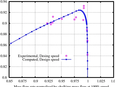
The procedure above was used to map the characteristic of the fan described in the previous section at three different aerodynamic speeds, namely 94%, 100% and 105% of the design speed. It is, once again, stressed that the only aerodynamic input quantities are the fan rotational speed and the nozzle areas. Of course, the ambient conditions can also be changed to study, for example, altitude effects but this is not the aim here. In any case, the fan characteristics obtained here are non-dimensionalised by the inlet conditions. Fig 13 shows the mass flow function versus pressure ratio for those three speeds where measured data is also shown for 100% speed (Sayma 2007). The agreement with measured data is very good, though it degrades slightly near the stall boundary. Two observations can be made on this issue. First, the numerical solution probably extends beyond the stall boundary of the measured characteristic, a feature that can be due to the “flow stability” provided by the numerical procedure. Circumferentially-averaged inter-blade-row boundary conditions do not allow for the propagation of circumferential disturbances that might eventually induce rotating stall in the actual test rig. Over-prediction of the stall boundary can also be observed in the NASA rotor 67 numerical predictions of the characteristic (Chima 1991).

It can also be observed also that there is a change in the shape of the characteristic as the stall boundary is approached, a feature that might be due to the running shape of the blade. In the analysis, the running shape of the blade was obtained at the working line and used along the speed characteristic. Since the shock position will change with speed, the blade running shape will also change due to different aerodynamic loads, leading to discrepancies observed in the computed characteristic. This feature can also be seen in the NASA rotor 67 prediction by Chima, 1991. It was reported by Wilson et al (2007) that the fan aerodynamic untwist varies along a speed characteristic between stall and choke. This variation can be significantly amplified at design speed and manufacturing tolerances variations from blade to blade need to be taken into account for accurate predictions.

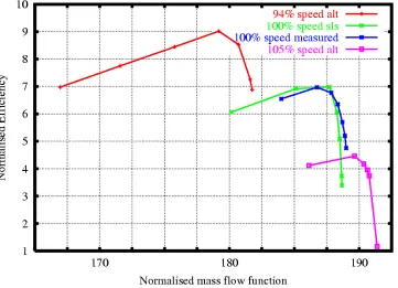
The predicted efficiency for the three speeds is shown in Fig 14, where the measured efficiency is also shown for 100% speed. Once again, there is good agreement with the predictions. Measured data for this fan are proprietary and the source cannot be published.

Further investigations in this study show that the predicted characteristic can vary according to the length of the extension behind the fan if an OGV is not introduced due to the variation of the swirl decay depending on the coarseness of the grid. Indeed if the grid was not coarse enough to remove the swirl, numerical instabilities appeared in the nozzle causing instabilities in the solution. These problems were completely removed by introducing the OGV and the solutions became independent of the extension of the domain ahead of the nozzle.

While it is observed here that the characteristic with the fan alone and with the fan, OGV and nozzle are the same, the advantages from the present approach stem from the following:

• Ability to sweep through the characteristic and speed without having to

change boundary conditions, mimicking the situation in actual rig tests.

• In situations where there are features that might affect the pressure rise in the

fan, such as the case with a bird strike for example, this approach provides a natural way of simulating the system. It allows the mass flow to respond to any blockage in the system without having to speculate what the exit pressure would be.

5.

Concluding remarks

• A modelling methodology was presented by which a fan characteristic was

mapped by sweeping along a speed characteristic or a long a working line in a single calculation without having to change boundary conditions. The approach resembles closely actual experimental fan characteristic mapping. This approach can be considered a significant step towards virtual testing of gas turbine engine compression systems.

• Whenever experimental data were available, comparisons were made;

particularly with the well documented NASA rotor 67 data. The agreement generally was good. Whenever some differences were observed, an explanation was given.

• If a nozzle is introduced behind a compressor rotor to control the downstream

throttle, it is important to remove the swirl from the flow before the nozzle instead of reducing the effect of the swirl numerically. The second approach could either lead to instabilities or inaccuracies in the simulations.

Acknowledgments

References

Chima, R. V. (1991) “Viscous three-dimensional calculations of transonic fan blades”, 77th symposium of propulsion and energetics panel: CFD techniques for propulsion applications, sponsored by AGARD, San Antonio, Texas, May 27-31 1991.

Fottner, L. ed. (1990), Test cases for computation of internal flows in aero engine

components, AGARD Advisory Report No. 275, AGARD, Neuilly-Sur-Seine, France, July 1990.

Sayma, A. I. (2007) “Steady flow analysis of low pressure compression system for turbofan engines”, ASME turbo expo 2007, Montreal, GT2007-27625, Canada 14-17 May 2007.

Sayma, A. I., Vahdati, M., Imregun M. and Marshall, J.G. (2007), “Low pressure compression system effects on fan assembly forced response” ASME turbo expo 2007, GT2007-27665, Montreal, Canada 14-17 May 2007

Sayma, A.I., Vahdati, M., Sbardella, L. and Imregun M. (2000) “Modelling of 3D viscous compressible turbomachinery flows using unstructured hybrid grids” AIAA ,Journal, 38(6), (2000), 945-954.

Sbardella, L., Sayma, A.I. and Imregun, M. (1999) “Semi-Unstructured Meshes for Axial Turbomachinery Blades” International Journal of Numerical Methods in Fluids. 32(5), (1999), 569-584.

Spalart, P. R., Allmaras, S. R., (1994), “A one-equation turbulence model for aerodynamic flows”, La Recherche Aerospatiale, 1, p 5ss. ( also AIAA paper 92-0439)

Strazisar, A.J., Wood, J. R., Hathaway, M. D. and Suder, K. L., (1989), “Laser anemometer measurements in a transonic axial flow fan rotor”, NASA TP-2879, Nov. 1989.

Vahdati, M., Sayma, A. I., Freeman, C. & Imregun, M. (2005) “On the use of atmospheric boundary conditions for axial-flow compressor stall simulations” Submitted to the ASME J of Turbomachinery, 127, (2005), 349-351.

Vahdati, M., Sayma A. I., Simpson, G. and Imregun, M. (2007) “Mulitbladerow Forced Response modelling in Axial-Flow Core Compressors”, ASME Journal of Tuebomachinery,129, (2007), 412-420

Wilson, M. (2006), The effect of blade variability in gas turbine fan assemblies, PhD thesis. Imperial College London.

Wu, X., Sayma, A. I., Vahdati, M. and Imregun. M. (2004) “Computational techniques for aeroelasticity and aeroacoustic analyses of aero-engine fan assemblies” International conference on fans, IMechE, London, Nov 2004

Figure 1 Solution domain for NASA rotor 67

Figure 4: Residual of the design speed characteristic sweep

Figure 6: Comparison of the characteristic with experimental data for NASA rotor 67

Figure 7: Mach number contours at 90% span for NASA rotor 67

Figure 9 : Comparison with rotor total pressure rise for NASA rotor 67

Figure 10: Comparison with rotor temperature rise for NASA rotor 67

Figure 12: Rotational speed sweep along a working line of NASA rotor 67