Bond-graph based substructuring of dynamical systems

White Rose Research Online URL for this paper:

http://eprints.whiterose.ac.uk/79694/

Version: Submitted Version

Article:

Gawthrop, P.J., Wallace, M.I. and Wagg, D.J. (2005) Bond-graph based substructuring of

dynamical systems. Earthquake Engineering and Structural Dynamics., 34 (6). 687 - 703.

ISSN 0098-8847

https://doi.org/10.1002/eqe.450

Reuse

Unless indicated otherwise, fulltext items are protected by copyright with all rights reserved. The copyright exception in section 29 of the Copyright, Designs and Patents Act 1988 allows the making of a single copy solely for the purpose of non-commercial research or private study within the limits of fair dealing. The publisher or other rights-holder may allow further reproduction and re-use of this version - refer to the White Rose Research Online record for this item. Where records identify the publisher as the copyright holder, users can verify any specific terms of use on the publisher’s website.

Takedown

If you consider content in White Rose Research Online to be in breach of UK law, please notify us by

P. J. Gawthrop

_{, M. I. Wallace}

_{and D. J. Wagg}

1_{Centre for Systems and Control and Department of Mechanical Engineering, University of Glasgow, GLASGOW. G12 8QQ}

UK

2_{Department of Mechanical Engineering, Queens Building, University of Bristol, Bristol BS8 1TR, UK.}

SUMMARY

A bond graph approach to hybrid simulation of dynamical systems using numerical-experimental real-time

substructuring is presented. The bond graph concepts of avirtual junctionand avirtual actuator, hitherto used

in the context of physical-model based control, are used to perform the substructuring in an intuitively appealing

way. The approach is illustrated by the reworking of a previously-published example.

The approach is verified experimentally using a bench-top multiple mass-spring system for the physical

substructure and automatically generated real-time code is used to implement the numerical substructure.

Copyright © 2004 John Wiley & Sons, Ltd.

KEY WORDS_{: Numerical-experimental substructuring; bond graphs; real-time control.}

∗_{Correspondence to: P. .J .Gawthrop, Centre for Systems and Control and Department of Mechanical Engineering, University of}

1. Introduction

This paper brings together two hitherto disparate research areas: real-time numerical-experimental

substructure-based testing of structures under dynamic loading as discussed by Wagg and Stoten [1]

and Darby et al. [2]; and bond graph based physical-model-based control as introduced by Sharon et al.

[3] and extended by Gawthrop [4], Costello and Gawthrop [5] and, in particular thevirtual actuator

approach of Gawthropet.al.[6,7].

Real-time dynamic substructuring is a novel experimental testing technique which can be used to

test individual components of engineering systems. This type of testing has been developed from

experimental testing of large scale structures using multiple time scales [8,9]. The basic concept is

that a complete model of the system is made by combining an experimental part with a numerical part.

Originally this was done for situations where numerical models of the experimental part were unreliable

— such as failure of concrete columns under earthquake loading [10]. However, the technique has now

been developed for a broader range of applications and in fact can now also be viewed as an advanced

form of component testing. In the fields of mechanical and aerospace engineering, physical components

are often tested to either characterise or improve the design performance. Substructure testing offers

a way of accurately testing nonlinear components which can be useful in many applications in these

fields. Some examples are described in [11] in connection with aerospace engineering. To carry out a

substructuring test the component of interest is isolated and fixed into an experimental test system. To

link the experimental substructure to the numerical substructure, a set oftransfer systemsare controlled

to follow the appropriate output from the numerical model. At the same time the forces between

the transfer systems and experimental substructure are fed back into the numerical model to give a

form bi-directional coupling. The key challenge is to carry out this operation effectively in real time

issue [14].

The bond graph approach to modelling of dynamic systems, introduced by Henry Paynter of MIT

[15], is well established [16,17, 18,19,20,21]. The authors believe that the approach provides a

natural conceptual framework for reasoning about substructuring.

As noted by Wagg and Stoten [1], the key issue of substructuring to be resolved is thesynchronisation

of the motion of the physical substructure and the computer-based numerical substructure. There

are two distinct problems here: the fact that the numerical integration implicit in the numerical

substructure introduces errors and the fact that there is usually a dynamical system (thetransfer system)

interposed between the computer and the physical systems. In this paper, the former is referred to as

the numerical synchronisation problem and the latter as thephysical synchronisationproblem. The

numerical synchronisationproblem is essentially an issue of numerical analysis. It has been discussed

by, for example, Darby et al. [2] and Algaard et al. [22]. Although important, it is not the subject of

this paper.

The physical synchronisation is essentially a control problem, with the response delay of the actuator

being the critical issue for the substructuring algorithm. Delay compensation is a well known issue for

real-time substructuring, with a number of single step forward prediction approaches having already

been presented by Horiuchi et al. [23], Darby et al. [13] along with other compensation techniques

such as Horiuchi and Konno [24] which have shown to improve accuracy. A more generic approach is

presented by Wallace et al. [14] which allows multiple and fractions of one time step to be predicted

without interpolation. Given the insight afforded by the bond graph approach, this paper shows that

an alternative solution to the physical synchronisation problem is provided by the virtual actuator

approach of Gawthropet.al.[6,7]. This method has the advantage that the virtual junction will provide

in principle, be used in the case when the substructure is nonlinear. However, within the context of this

paper, the virtual junction approach is applied to linear substructured systems.

The paper is organised as follows. Section 2 gives a bond graph based interpretation of

substructuring. Section3introduces virtual junctions and actuators and section4illustrates the method

using a previously used example [1]. Section5discusses an experimental verification of the approach,

and Section6concludes the paper and discusses some possible extensions.

2. Bond Graph Substructuring

F

N

v

N

F

P

v

P

Phy

Num

(a) Model

aPhy

aNum

u

F

P

(b) Augmented Model

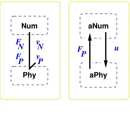
Figure 1. Substructuring

Following Wagg and Stoten [1] and Darby et al. [2], this paper considers real-time dynamic

substructuring whereby a dynamic system issubstructuredinto two parts:

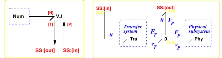
Num SS:[in] [1,2] SS:[out] [1,2] VJ [N] [T] [P] (a) Numerical F_P v P F P 0 v T F_T u Physical subsystem Transfer system 0 SS:[out] [1,2] [1,2] Phy Tra SS:[in] [1,2] (b) Physical

Figure 2. Augmented substructures

physical substructure to be implemented physically.

Substructuring can be readily described in bond graph terms as follows. Given the bond graph of a

dynamic system, choose the set of components forming the physical substructure and mark all bonds

external to this substructure, in general there will beN≥1 such bonds and the remaining components

will form the numerical substructure. Thus each of the two substructures hasNports connected by the

Nmarked bonds. In the case of mechanical systems, each port will correspond to a force-velocity pair;

in general this can be any effort-flow pair.

This decomposition is depicted in Figure1(a) whereNumandPhyare the numerical and physical

substructures respectively. FN and vN are the force/velocity pair associated with the numerical

substructure andFPandvPare the force/velocity pair associated with the physical substructure. The

connecting bond implements the twointerface equations:

        

FP =FN

vP =vN

(1)

and thus both the numerical and physical substructures may themselves contain many subsystems. In

this case, the quantities in (1) can be regarded as vectors containingN components. The simulation

example of Section4hasN=1; the experimental example of Section5hasN=2.

As pointed out previously, [1, 2] it is often not possible to connect the two substructures of

Figure1(a) because it is not physically possible to directly apply the signal implied by the numerical

substructure to the physical system. In bond graph terms, the two systems of Figure 1(a)cannot

be connected via an energy bond; as indicated in Figure 1(b),augmented versions of the numerical

(aNum) and physical (aPhy) substructure are connected using a pair of active bonds. For the purposes

of this paper it is assumed that:

Assumption 1. The causality is such that thephysicalsubstructure in Figure1(a) imposes aforce(in

general effort) on thenumericalsubstructure.

Assumption 2. The quantity imposed by the physical substructure in Figure 1(a) can be directly

measured.

Assumption 3. The quantity imposed by thenumericalsubstructure of Figure1(a) cannot be directly

imposed on thephysicalsubstructure but rather via an N-input utransfer system. In particular, the

input u can only be imposed via atransfer systemlabelledTra_{in Figure2(b).}

Assumption1is not essential but simplifies the development; assumption2is essential for this paper

but could be removed as discussed in Section6; assumption3is the main issue addressed here.

The fact that the substructured system of Figure1(a) cannot be directly implemented but rather must

be approximated by Figure1(b) means that (1) no longer holds and must be replaced by:

    

   

FP−FN =F˜

vP−vN =v˜

where ˜F is the force synchronisation error and ˜v is the velocity synchronisation error. The

synchronisation problem is to reduce the two synchronisation errors to acceptable values; exact

synchronisation†corresponds to

    

   

˜

F =0

˜

v =0

(3)

A similar problem has been noted in the context of bond graph based physical-model based

control [6, 7]. This paper applies the (suitably modified) solution of this control problem to the

substructuring problem. In particular, it is shown constructively in Section 3 that if the augmented

physical substructure aPhy of Figure 1(b) is given by Figure 2(a), then the three-port (each port

corresponding to N bonds) virtual junction VJcomponent can, in certain circumstances, provide a

solution to theexact synchronisationproblem.

3. Virtual junctions and Actuators

The virtual actuatorapproach to control system design was introduced by Gawthrop et al. [6] and

experimentally verified by [7] in the context of control system design. The same concepts are used in

this paper in the context of substructuring; this section gives a brief overview of the approach.

The virtual junction component appearing in Figure1(b) has three ports labelled:

[P ], carrying the measured signalyfrom thephysicalsystem but imposing 0 signal onto the physical

system;

[T ], carrying the control signaluto the input of thetransfersystem but not carrying any measurement

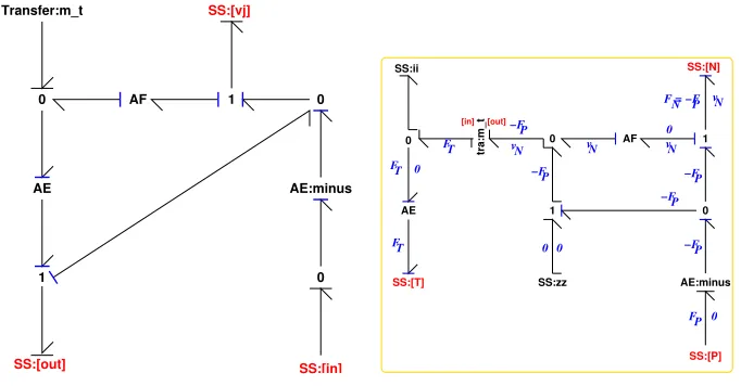
SS:[in] SS:[out] SS:[vj] AE:minus Transfer:m_t 0 0 1 AF AE 1 0 (a) Collocated

−F _P

F _P −F _P −F _P F = −F_{N P vN}

vN vN

v N −F _P −F _P

FT FT FT 0 0 0 0 0 SS:[N] [out] [in] SS:[T] SS:[P] AE:minus tra:m_t SS:zz SS:ii 1 AF 0 1 0 AE 0 (b) Non-collocated

Figure 3. Virtual Junction: bond graph

and

[N ] the port to which the numerical system is attached.

The purpose of the virtual junction is to make the input-output properties of the systems of Figure1(a)

and1(b) identical. For example, this can be done if the virtual junction implements the equations:

    FN FT     =    

−1 0

1 T−1

        FP vN     (4)

wherevT =T FT.

The design of the virtual junction component is considered in detail elsewhere [7,6]. The design for

a particular example is discussed in Section4. Given the structure of Figure1, there are two restrictions

on the class of systems for which a virtual junction can be successfully implemented:

Assumption 5. Definingσ_{N as the length of the shortest causal path (SCP) between FN and vN and}

σ_{T as the length of the SCP between FT and vT, then:}

σ_N≥σ_{T (5)}

Assumption 4 ensures internal stability and assumption 5 ensures that the combined numerical

substructure and virtual junction is proper and thus has a state-space realisation.

It is clear from this that an accurate model of thetransfersystem is required. Section5 has more

discussion on this point.

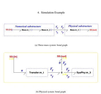
4. Simulation Example

F_N

v_N F_P

v_P

Physical substructure Numerical substructure

SS:[in] Mass:m_1 Mass:m_2 Mass:m_3 SS:[out]

(a) Three-mass system: bond graph

v

F

T

F

v

u

F

0

0 SysPhy:m_3

SS:[out]

Transfer:m_t

SS:[in]

[1,2] [1,2]

[1,2]

(b) Physical system: bond graph

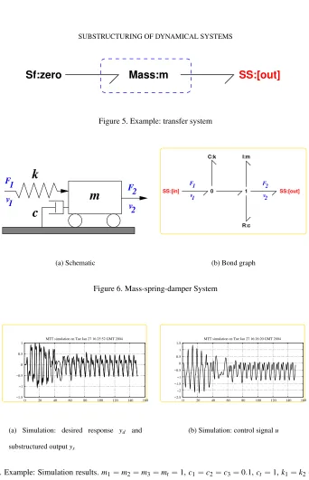
Mass:m

Sf:zero

SS:[out]

Figure 5. Example: transfer system

F 2 v2 F 1

v1

m

k

c

(a) Schematic

F 1 v1

F 2 v2

SS:[in] 0 1 SS:[out]

C:k I:m

R:c

(b) Bond graph

Figure 6. Mass-spring-damper System

−1.5 −1 −0.5 0 0.5 1

0 20 40 60 80 100 120 140 160 MTT simulation on Tue Jan 27 16:25:52 GMT 2004

(a) Simulation: desired response yd and

substructured outputys

−2.5 −2 −1.5 −1 −0.5 0 0.5 1 1.5

0 20 40 60 80 100 120 140 160 MTT simulation on Tue Jan 27 16:26:20 GMT 2004

(b) Simulation: control signalu

Figure 7. Example: Simulation results.m1=m2=m3=mt=1,c1=c2=c3=0.1,ct=1,k1=k2=kt=1,

k3=₋1+δ2whereδis the spring extension.r=₋0_.5 sin(t)

Wagg and Stoten [1] consider substructuring in the context of a three mass-spring-damper system

three instances of theMasscomponent depicted in Figure6. In the example of Wagg and Stoten [1] ,

the third mass (m3in Figure4) is a physical system whereas the other two masses (m1&m2in Figure

4) are to be realised by numerical simulation. Causal strokes have been added to show that, in this case,

Assumption1holds.

Further, with reference to Figure4(b) the physical massm3is controlled via thetransfer system mt.

As shown in Figure5, theTransfersystem is based on theMasssubstructure with the left-hand port

connected to a zero velocity source. This gives a simpler situation than that of Figure1as bothFT and

vT are associated with a single port.

Following the approach of Section2, the numerical system is obtained as in Figure2(a) by attaching

the masses m1 &m2 to the virtual junctionwhich is shown in expanded form in 3(a). The virtual

junction transfer function representation is:

    FN FT     =    

−1 0

1 (cts+kt+mts

2₎ s         FP VN     (6)

The overall system then consists of thenumericalandphysicalsystems connected as in Figure1.

As discussed in Section 2, the numerical simulation corresponds to aproper transfer function. The

corresponding state-space matrices are:

A=                

0 (−1)

m₁ 0 0 0

k1 (−

c₁₎

m1 −k2 0 0

0 m11 0

(−1)

m2 0

0 0 k2 (−

c₂)

m2 0

0 0 0 m1₂ 0

B=                 0 1 0 0 0 0

−1 0

0 0                 (8) C= µ

0 0 (k2mt) m₂

(−c2mt+ctm2) m2₂ kt

¶

(9)

D=

µ

(m2−mt)

m₂ 0

¶

(10)

The desired system of Figure4(a) and the substructured system of Figure 1were both simulated

using the numerical parameters indicated in Figure7and the velocity of the third mass of the desired

system (yd), together with the corresponding velocity of the third mass of the substructured system (ys),

are plotted in Figure7(a). There is a transient error due to a non-zero initial condition being applied

to the transfer system (initial velocity = 0.01). With zero initial conditions,ys=yd. Figure7(b)shows

the control signal associated with the substructured system: the external force applied to the transfer

system. The simulation code was automatically generated from the bond graph diagrams using MTT

2 X k1

c1

k2

c2 v1

F1

v2 F2

X 1

k

n2

c

n2

m

m

3

k

c

n1

m

Numerical

Physical

Numerical

Figure 8. Physical/Numerical Substructured system.kn1=kn2=k1=k2=4750Nm−1;cn1=cn2=c1=c2=

6Nsm−1_;m

n1=mn2=m3=6Nsm−1.

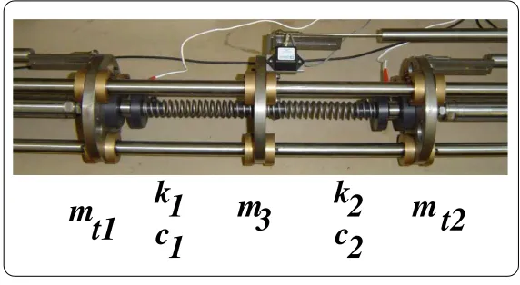
m

t1

k1

_c1

m3

k2

_c2

m t2

Figure 9. Augmented Physical substructure: Photo

5. Experimental Example

The model to be simulated appears in Figure 8; it has been divided into physical and numerical

substructures and the parameters are given in the caption. The physical substructure is modelled as

Figure10. Thus the substructured model corresponding to this example appears in Figure1(a) where

both the numerical and physical substructures have been vectorised withN=2.

Figure9shows the substructured three mass system. The physical substructure is the central mass

F1 v1

k1

c1

k2

c2 F2 v2

m

(a) Schematic

v1

F1 F2

v2

SS:[L] 1

I:m

0 1

R:c_1

0 1

R:c_2 C:k_2

SS:[R] C:k_1

INTF De:y

(b) Bond graph

SS:[in_1] [L]Mass2:m_3[R] SS:[in_2]

(c) Vector bond graph

Figure 10. A two-port system

SS:[in] 1 SS:[out]

I:m

R:c 1

C:k

AE:ae

(a)tracomponent bond graph

SS:[in_1] tra:m_t1 SS:[out_1] SS:[in_2] tra:m_t2 SS:[out_2]

(b) Bond graph

Figure 11. Experimental example: Transfer system (Tra₎

springk1and another between the massmt2and the springk2. The left-hand massmt1, together with

the actuator, forms the scalar transfer systemtraof Figure11(a); two instances oftraare combined in

To implement real-time substructuring we are using a dSpace DS1104 R&D Controller Board

running on hardware architecture of MPC8240 (PowerPC 603e core) at 250 MHz with 32 MB

synchronous DRAM (SDRAM). This DSP type board offers 4 A/D channels at 16 bit, 4 A/D

channels at 12 bit with 8 D/A channels at 16 bit, of which 5 and 4 are required respectively for

this substructuring example. This is fully integrated into the block diagram-based modelling tool

MATLAB™/Simulink™which is used to build the substructuring model. The dSpace companion

software ControlDesk is used for online analysis and control, providing soft real-time access to the

hard real-time application.

Simulink™s-functions were automatically generated from the bond graph representation of the

augmented numerical substructureaNumof Figures1(b)and2(a)using the MTT [25] package.

Two UBA (timing belt and ball screw configuration) linear Servomech actuators are used as the

transfer systems, with maximum force capacity of 500N and maximum linear speed of 640mms−1_.

These are driven independently by two Panasonic Minas Series AC servo motors which are configured

as analogue amplifiers to remove any internal closed loop control functions. Three RDP Electronics

DCT captive guided DC LVDT displacement transducers are used to measure the displacement of

the two transfer systems and the substructure which have a ±0.11% linearity error on full scale

deflection of 50mm. Each unit has an internal bearing that guides the armature built-in DC to

DC signal conditioning to help remove noise. Two RDP Electronics model 31 precision miniature

tension/compression load cells are used for the force measurements either side of the substructure.

The unit is applicable both in tension and compression with linearity±0.15%, hysteresis±0.15% and

non-repeatability±0.1% of full scale deflection. Each mass is a constant 2.2kg and connected to the

rig via three parallel shafts constraining their motion to one degree of freedom with an axial alignment

plates to reduce friction. Through system identification the spring constants were found constant for

all and equal tok=4750Nm−1

and damping ratio ofc=6Nsm−1

.

There were two sets of experiments: identification of a dynamical model of the transfer system

(Section5.1) and validation of the bond graph approach to substructuring (Section5.2).

5.1. Transfer system identification

The left-hand transfer system has the following components:

1. the linear actuator, comprising an AC servo motor and associated power amplifier driving a

ball-screw mechanism;

2. the massmt1of Figure9, equal to 2.2 kg;

3. the LVDT sensor measuring the positionx1of the massmt1

The right-hand transfer system was similar.

As discussed in section 3, the virtual junction approach requires an accurate model of the transfer

system. Unfortunately, AC servos are non-linear [26] and difficult to characterise from first principles

as is the ball screw mechanism. Analysis of experimental measurements of step responses showed that

the dynamical response of the servo motor/ball-screw was indeed dependent on the form of the input

signal.

Most actuators used in this context are indeed non-linear and this must therefore be an important

consideration in transfer system design. In particular, it is well-known that the use of feedback reduces

uncertainly and nonlinearity. For this reason, a variable-gain proportional digital controller with gain

g1, sample interval∆=1ms, setpointxd1and described by

was implemented whereu1is the input to the linear actuator1. Theclosed-looptransfer system was

observed to have a more linear response than the open-loop transfer system.

−0.2 0 0.2 0.4 0.6 0.8 1 1.2 1.4

0 0.02 0.04 0.06 0.08 0.1 0.12 0.14 0.16 0.18 0.2

Displacement

Time Closed−loop displacement step response

(a)xt1forg1=0.6,0.8,1.0

−0.2 0 0.2 0.4 0.6 0.8 1 1.2 1.4

0 0.02 0.04 0.06 0.08 0.1 0.12 0.14 0.16 0.18 0.2

y

t Comparison of data

(b)xt1& ˆxt1forg1=1.0

Figure 12. Identified transfer system step responses

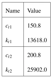
Name Value

ct1 150.8

kt1 13618.0

ct2 200.8

kt2 25902.0

Table I. Estimated Parameters

Sequences of input (xd1) and output (x1) data were measured when the mass was disconnected from

the springk1for three values ofg1. Using the “frequency-sampling filter” method of Wang and Cluett

[27], a step response (relatingxd1andx1) was identified for each of the three values of gain and plotted

in Figure 12(a). Although the bond graph of Figure 11does not correspond in detail to the actual

transfer system, it isphysically plausiblein the sense of Gawthrop [28] and so its parameters can be

estimated using the sensitivitybond graph approach [29]. The massmt1is known, and so the two

must repeat this identification for the right hand transfer system as its frictional characteristics are not

necessarily the same regardless of its mechanical similarity. In fact it can be seen from TableIthat the

dynamics from Transfer System 2 are quite different.

The step responses of this physically plausible model are compared with the data-based step response

of12(a) forg1=1.0 in Figure12(b). The match is not perfect, but the identified model was used for

the experiments of Section5.2.

5.2. Experimental validation

Synchronisation subspaceplots are used to show the effectiveness of the control algorithm by plotting

the desired verses actual responses, [30]. A subspace plot shows the amplitude accuracy and the

magnitude of delay coupled together at any one time interval. Perfect synchronisation is represented

by a straight line at an angle of 45◦_{to the horizontal with maxima and minima of the reference signal.}

Any reduction in synchronisation can be seen as a deviation from this idealised line. The result of

varying the amplitude accuracy is to change the angular orientation of the subspace plot compared to

the idealised line whereas a constant delay between the reference signal and the response results in

transforming the idealised straight line into an ellipse.

For constant wall excitation conditions these plots builds up into a repeating periodic pattern, which

can appear complex. However, the individual components of amplitude and delay produce their own

specific and identifiable patterns if evaluated separately. We use subspace plots as they allow the

controller effectiveness to be characterised in an online procedure, important for real-time testing,

and displays far more information than can be interpreted from simply observing the error between the

two signals.

−2 −1 0 1 2 −1.5 −1 −0.5 0 0.5 1 1.5

(b) TS 1 − NM and Virtual Junction

Amplitude (cm)

Amplitude (cm)

−2 −1 0 1 2

−1.5 −1 −0.5 0 0.5 1 1.5

(d) TS 2 − NM and Virtual Junction

Amplitude (cm)

Amplitude (cm)

−2 −1 0 1 2

−1.5 −1 −0.5 0 0.5 1 1.5

(a) TS 1 − NM only

Amplitude (cm)

Amplitude (cm)

−2 −1 0 1 2

−1.5 −1 −0.5 0 0.5 1 1.5

(c) TS 2 − NM only

Amplitude (cm)

Amplitude (cm)

z₂ vs x₂ Idealised Line z₂ vs x₂

Idealised Line

z₁ vs x₁ Idealised Line z₁ vs x₁

Idealised Line

Figure 13. Wall excitation ofr1=5Hzandr2=5Hz.

synchronisation, theactualdisplacement of the transfer system,xi, must be equal to thedesiredoutput

from its respective numerical model (NM),zi, wherei=1,2 according to the transfer system being

observed. Figure13shows the results of both transfer systems for a sinusoidal excitation of 5Hzfrom

each wall,r1andr2. We compare the effectiveness of the control algorithm when the virtual junction

is included in the numerical model, (b)and(d), to when there is no plant model included, (a)and

(c). We can clearly see that the constant phase delay caused by the mechanical characteristics of each

−2 −1 0 1 2 −2 −1.5 −1 −0.5 0 0.5 1 1.5

2 (b) TS 1 − NM and Virtual Junction

Amplitude (cm)

Amplitude (cm)

−1 −0.5 0 0.5 1

−1 −0.5 0 0.5

1 (d) TS 2 − NM and Virtual Junction

Amplitude (cm)

Amplitude (cm)

−2 −1 0 1 2

−2 −1.5 −1 −0.5 0 0.5 1 1.5

2 (a) TS 1 − NM only

Amplitude (cm)

Amplitude (cm)

−1 −0.5 0 0.5 1

−1 −0.5 0 0.5

1 (c) TS 2 − NM only

Amplitude (cm)

Amplitude (cm)

z₁ vs x₁ Idealised Line

z₁ vs x₁ Idealised Line

z₂ vs x₂ Idealised Line

z₂ vs x₂ Idealised Line

Figure 14. Wall excitation ofr1=3Hzandr2=5Hz.

systems. Comparing the shape of the subspace plots(a)and(c)we can see that although the transfer

systems are the same type of actuator they have slightly differing mechanical properties due to differing

frictional characteristics as predicted by the transfer system identification in Section5.1. This is why

we must use a separate model for each transfer system in its respective virtual junctions to account for

these mechanical variations.

The transfer system models are found though the system identification process as described in

of the control algorithm a feed-forward process, which means that the plant cannot not be subject to

frequency dependant behaviour. Figure14shows the results when the wall excitations are not equal and

opposite, thus the transfer systems must now be controlled to a compound sinusoid. We can see from

(b)and(d)that again the inclusion of the virtual junction has a beneficial effect on the synchronisation

compared to when just the simple numerical model is used,(a)and(c), but not to such a same extent

as in Figure13. This is due to the the transfer system models loosing coherence at the low frequencies.

We can also see this when we introduce a sinusoidal sweep as the wall inputs. Figure15shows the case

where we have a sweep from 1Hzto 5Hzfor the left hand wall excitation,r1, and a sweep from 3Hzto

4Hzfor the right hand wall excitation,r2. Although we again see a much higher level of synchronisation

when the virtual junction is included in the numerical model,(b)and(d), we cannot achieve the high

level of coherence as seen from Figure13, again due to the frequency dependent characteristics of the

transfer systems.

We can see from these results that the phase inversion achieved by the virtual junction has a

significant effect on increasing the synchronisation of the transfer systems. However, to increase its

effectiveness over the whole plant frequency range the transfer system models could be replaced by

an on-line system identification. This would close the control loop round the phase inversion stage of

the virtual junction and make the it possible to achieve high levels of synchronisation for compound

sinusoids caused by out of phase wall excitations.

6. Conclusions

A bond graph approach to real-time numerical-physical substructuring has been introduced which not

only gives new insight into substructuring but also provides a solution to the problem of synchronising

−1.5 −1 −0.5 0 0.5 1 1.5 −1.5 −1 −0.5 0 0.5 1

1.5 (b) TS 1 − NM and Virtual Junction

Amplitude (cm)

Amplitude (cm)

−2 −1 0 1 2

−2 −1.5 −1 −0.5 0 0.5 1 1.5

2 (d) TS 2 − NM and Virtual Junction

Amplitude (cm)

Amplitude (cm)

−1.5 −1 −0.5 0 0.5 1 1.5 −1.5 −1 −0.5 0 0.5 1

1.5 (a) TS 1 − NM only

Amplitude (cm)

Amplitude (cm)

−2 −1 0 1 2

−2 −1.5 −1 −0.5 0 0.5 1 1.5

2 (c) TS 2 − NM only

Amplitude (cm)

Amplitude (cm)

z₂ vs x₂ Idealised Line z₂ vs x₂

Idealised Line

z₁ vs x₁ Idealised Line z₁ vs x₁

Idealised Line

Figure 15. Wall sine sweep excitation ofr1= 1 to 5Hz andr2= 3 to 4Hz in 60 seconds.

The experimental results highlighted the need for an accurate model of the transfer system. Three

techniques were used to achieve this: feedback control to reduce non-linearity and the effect of

poorly-known parameters; bond graph modelling to give physical insight and system identification to tune

physical parameters.

There are a number of topics that will be the subject of further investigation by the authors:

Transfer system design In the light of the experiments reported here, future work will pay close

non-linear modelling and control system design will be investigated. Once again, the bond graph approach

can be used not only for modelling and control design but also for actuator sizing [31,32,33].

Virtual sensors Sections2 and4assumes that the output of the physical system (in this caseFP)

is available for measurement. If this is not the case, or the measurement is badly corrupted by noise,

then thevirtual sensor approachmay be used. This has been previously used in the context of Physical

Model Based Control [4,34] and is based on the bond graph analogue to an observer or Kalman

filter[35].

Backstepping The relation between the bond graph approach and the backstepping approach of

Krstic et al. [36] was noted by [37,38]. The relationship with the virtual actuator approach is noted by

[6,7]. A non-bond graph approach based on backstepping is therefore a possibility.

On-line System Identification The Experimental validation section,5.2, highlights the need for the

models of the transfer systems to be calculated in an on-line system identification procedure. If this can

be achieved as part of the numerical model stage then frequency dependent behaviour and changing

plant conditions could be effectively controlled.

Non-Linear Substructure The ability to test to non-linear substructures would enable more realistic

structures to be investigated moving towards real industrial applications. Additionally, a non-linear

substructure will highlight the difficulties experienced due to cross-coupling between the transfer

systems in multi degree of freedom substructuring.

ACKNOWLEDGEMENTS

and David Wagg via an EPSRC Advanced Research Fellowship. Geraint Bevan (Glasgow University) wrote the

s-function generation code for MTT.

references

[1] D.J. Wagg and D.P. Stoten. Substructuring of dynamical systems via the adaptive minimal control approach.

Earthquake Engng Struc. Dyn., 30(6):865–877, June 2001.

[2] A. P. Darby, A. Blakeborough, and M. S. Williams. Improved control algorithm for real-time substructure

testing.Earthquake Engng Struc. Dyn., 30(3):431–448, March 2001.

[3] A. Sharon, N. Hogan, and D. E. Hardt. Controller design in the physical domain. Journal of the Franklin

Institute, 328(5):697–721, 1991.

[4] P. J. Gawthrop. Physical model-based control: A bond graph approach. Journal of the Franklin Institute,

332B(3):285–305, 1995.

[5] Des J. Costello and Peter J. Gawthrop. Physical-model based control: Experiments with a stirred-tank heater.

Trans. IChemE, Part A, 27:361–370, March 1997.

[6] Peter J Gawthrop, Donald J Ballance, and Dustin Vink. Bond graph based control with virtual actuators. In

Norbert Giambiasi and Cluadia Frydman, editors,Proceedings of the 13th European Simulation Symposium:

Simulation in Industry, pages 813–817, Marseille, France, October 2001. SCS. ISBN 90-77039-02-3.

[7] Peter J Gawthrop. Bond graph based control using virtual actuators. Proceedings of the Institution of

Mechanical Engineers Pt. I: Journal of Systems and Control Engineering, 218(4):251–268, September 2004.

URLhttp://dx.doi.org/10.1243/0959651041165864.

[8] M. Nakashima, H. Kato, and E. Takaoka. Development of real-time pseudo dynamic testing. Earthquake

Engineering and Structural Dynamics, 21:779–92, 1992.

[9] J. Donea, P. Magonette, P. Negro, P. Pegon, A. Pinto, and G. Verzeletti. Pseudodynamic capabilities of the

[10] Yu-Yuan Lin, Kuo-Chun Chang, and Yuan-Li Wang. Comparison of displacement coefficient method and

capacity spectrum method with experimental results of rc columns.Earthquake Engineering and Structural

Dynamics, 33(1):35–48, 2004.

[11] M. S. Williams and A. Blakeborough. Laboratory testing of structures under dynamic loads: an introductory

review.Philosophical Transactions of the Royal Society A, 359:1651 – 1669, 2001.

[12] A. Blakeborough, M. S. Williams, A. P. Darby, and D. M. Williams. The development of real-time

substructure testing.Philosopical Transactions of the Royal Society of London A, 359:1869–1891, 2001.

[13] A. P. Darby, A. Blakeborough, and M. S. Williams. Real-time substructure tests using hydraulic actuator.

Journal of Engineering Mechanics, 125(10):1133–1139, 2001.

[14] M. I. Wallace, D. J. Wagg, and S. A. Neild. A polynomial based forward prediction algorithm for improving

the accuracy of real-time dynamic substructuring.Submitted to Proceedings of the Royal Society A, 2004.

[15] H. M. Paynter. Analysis and design of engineering systems. MIT Press, Cambridge, Mass., 1961.

[16] Peter J Gawthrop and Serge Scavarda. Special issue on bond graphs: Editorial.Proceedings of the Institution

of Mechanical Engineers Pt. I: Journal of Systems and Control Engineering, 216(I1):i–v, March 2002. URL

http://dx.doi.org/10.1243/0959651021541363.

[17] Dean Karnopp, Donald L. Margolis, and Ronald C. Rosenberg.System Dynamics : Modeling and Simulation

of Mechatronic Systems. Horizon Publishers and Distributors Inc, 3rd edition, January 2000.

[18] Amalendu Mukherjee and Ranjit Karmakar. Modelling and Simulation of Engineering Systems through

Bondgraphs. Alpha Science, 2000.

[19] P. J. Gawthrop and L. P. S. Smith.Metamodelling: Bond Graphs and Dynamic Systems. Prentice Hall, Hemel

Hempstead, Herts, England., 1996. ISBN 0-13-489824-9.

[20] Lennart Ljung and Torkel Glad.Modeling of Dynamic Systems. Prentice Hall, 1994.

[22] W. Algaard, A. Agar, and N. Bicanic. Enhanced integral form of the Newmark time stepping scheme for

pseudodynamic testing.Engineering Computations, 18(3):676–689, 2001.

[23] T. Horiuchi, M. Inoue, T. Konno, and Y. Namita. Real-time hybrid experimental system with actuator delay

compensation and its application to a piping system with energy absorber. Earthquake Engineering and

Structural Dynamics, 28:1121–1141, 1999.

[24] Toshihiko Horiuchi and Takao Konno. A new method for compensating actuator delay in real-time hybrid

experiments.Philosophical Transactions of the Royal Society A, 359:1893 – 1909, 2001.

[25] MTT. MTT: Model transformation tools. Online WWW Home Page, 2002. URL: http://mtt.sourceforge.net.

[26] P.C. Sen. Principles of Electrical Machines and Power Electronics. John Wiley, 2nd edition, 1997.

[27] L Wang and W R Cluett. From Plant Data to Process Control. Taylor and Francis, London and New York,

2000.

[28] Peter J Gawthrop. Physically-plausible models for identification. InProceedings of the 2003 International

Conference On Bond Graph Modeling and Simulation (ICBGM’03), Simulation Series, Orlando, Florida,

U.S.A., January 2003. Society for Computer Simulation.

[29] Peter J Gawthrop. Sensitivity bond graphs. Journal of the Franklin Institute, 337(7):907–922, November

2000. URLhttp://dx.doi.org/10.1016/S0016-0032(00)00052-1.

[30] P. Ashwin. Non-linear dynamics, loss of synchronization and symmetry breaking. Proceedings of the

Institution of Mechanical Engineers, Part G: Journal of Aerospace Engineering, 212(3):183–187, 1998.

[31] Roger F Ngwompo and Peter J Gawthrop. Bond graph based simulation of nonlinear inverse systems using

physical performance specifications. Journal of the Franklin Institute, 336(8):1225–1247, November 1999.

URLhttp://dx.doi.org/10.1016/S0016-0032(99)00032-0.

[32] Ngwompo R F, Scavarda S, and Thomasset D. Physical model-based inversion in control systems design

using bond graph representation part 1: theory.Proceedings of the I MECH E Part I Journal of Systems and

[33] Ngwompo R F, Scavarda S, and Thomasset D. Physical model-based inversion in control systems design

using bond graph representation part 2: applications.Proceedings of the I MECH E Part I Journal of Systems

and Control Engineering, 215(2):105–112, April 2001.

[34] Peter J. Gawthrop and Donald J. Ballance. Symbolic algebra and physical-model-based control.Computing

and Control Journal, 8(2):70–76, April 1997. ISSN 0956-3385.

[35] D. C. Karnopp. Bond graphs in control: Physical state variables and observers.J. Franklin Institute, 308(3):

221–234, 1979.

[36] M. Krstic, I. Kanellakopoulos, and P. V. Kokotovic. Nonlinear and Adaptive Control design. New York:

Wiley, 1995.

[37] T-J Yeh. Backstepping design in the physical domain. InProceedings of the American Control Conference,

1999.