Terrain analysis using radar shape-from-shading

This is a repository copy of

Terrain analysis using radar shape-from-shading

.

White Rose Research Online URL for this paper:

http://eprints.whiterose.ac.uk/945/

Article:

Bors, A G orcid.org/0000-0001-7838-0021, Hancock, E R orcid.org/0000-0003-4496-2028

and Wilson, R C orcid.org/0000-0001-7265-3033 (2003) Terrain analysis using radar

shape-from-shading. IEEE Transactions on Pattern Analysis and Machine Intelligence. pp.

974-992. ISSN 0162-8828

https://doi.org/10.1109/TPAMI.2003.1217602

[email protected] https://eprints.whiterose.ac.uk/ Reuse

Items deposited in White Rose Research Online are protected by copyright, with all rights reserved unless indicated otherwise. They may be downloaded and/or printed for private study, or other acts as permitted by national copyright laws. The publisher or other rights holders may allow further reproduction and re-use of the full text version. This is indicated by the licence information on the White Rose Research Online record for the item.

Takedown

If you consider content in White Rose Research Online to be in breach of UK law, please notify us by

Terrain Analysis Using

Radar Shape-from-Shading

Adrian G. Bors,

Member,

IEEE, Edwin R. Hancock, and

Richard C. Wilson,

Member,

IEEE Computer Society

Abstract—This paper develops a maximum a posteriori (MAP) probability estimation framework for shape-from-shading (SFS) from synthetic aperture radar (SAR) images. The aim is to use this method to reconstruct surface topography from a single radar image of relatively complex terrain. Our MAP framework makes explicit how the recovery of local surface orientation depends on the whereabouts of terrain edge features and the available radar reflectance information. To apply the resulting process to real world radar data, we require probabilistic models for the appearance of terrain features and the relationship between the orientation of surface normals and the radar reflectance. We show that the SAR data can be modeled using a Rayleigh-Bessel distribution and use this distribution to develop a maximum likelihood algorithm for detecting and labeling terrain edge features. Moreover, we show how robust statistics can be used to estimate the characteristic parameters of this distribution. We also develop an empirical model for the SAR reflectance function. Using the reflectance model, we perform Lambertian correction so that a conventional SFS algorithm can be applied to the radar data. The initial surface normal direction is constrained to point in the direction of the nearest ridge or ravine feature. Each surface normal must fall within a conical envelope whose axis is in the direction of the radar illuminant. The extent of the envelope depends on the corrected radar reflectance and the variance of the radar signal statistics. We explore various ways of smoothing the field of surface normals using robust statistics. Finally, we show how to reconstruct the terrain surface from the smoothed field of surface normal vectors. The proposed algorithm is applied to various SAR data sets containing relatively complex terrain structure.

Index Terms—Synthetic aperture radar imagining, shape-from-shading, terrain surface reconstruction, maximum a posteriori probability estimation, robust statistics.

æ

1

I

R

recovering terrain topography from synthetic aperture radar (SAR) images. It was the need to develop techniques for mapping the surface of planet Venus from Magellan imagery that has stimulated research in the area [1]. Due to the nature of the radar image acquisition process, the task of interpreting SAR images poses a number of challenges. Such problems are caused by the complex physics of radiation-material interac-tion, the radar beam, wavelength, variations due to the vegetation, level of humidity, type of terrain, foreshortening, layover, shadowing, man-made objects, or the process of radar image acquisition [2], [3], [4], [5], [6], [7], [8], [9], [10]. The study of terrain SAR images is termed radarclinometry and has been shown to provide a powerful means of probing three-dimensional structure [9], [11], [12], [13], [14], [15], [16], [17]. Although there are a number of well-developed methods for recovering three-dimensional surface structure from multiple radar images, there is relatively little work aimed at terrain analysis from single SAR images. In the computer vision literature, the pioneering work on the subject was performed by Frankot and Chellappa [11], who extended the Lambertian shape-from-shading method of Ikeuchi and Horn [18] to radar reflectance. One of the important features of the method was the way in which it imposed integrability constraints on surface reconstruction in the Fourier domain.

Despite the significant effort in the area, one of the shortcomings of existing work is its lack of a statistical basis. This is an important omission since radar data is notor-iously noisy. Hence, the aim in this paper is to develop a statistical framework for radar shape-from-shading. Speci-fically, we develop a maximum a posteriori probabilistic framework, which allows surface normals to be estimated using a model of the radar reflectance function and an estimate of the whereabouts to ridge and ravine structures in the terrain under study. In the remainder of this section, we review the related literature in more detail and outline the main novelty of our contribution.

1.1 Related Literature

One of the classical approaches to SFS was the regularization method introduced by Ikeuchi and Horn [18] and later extended and developed by Horn and Brooks [19]. According to the regularization framework, the field of surface normals is iteratively updated so as to minimize a brightness error subject to local smoothness constraints. The main limitation of this approach is the need to balance the effects of brightness and smoothness errors while adjusting the surface normal directions. Specifically, it has a marked tendency to over-smooth the surface normals and erode fine surface detail. Recently, Worthington and Hancock [20] have attempted to remedy this problem by imposing the image irradiance equation as a hard constraint. According to their approach, the surface normals are constrained to always lie on a cone whose apex angle is determined by the image brightness and whose axis is in the light source direction. There are many alternative approaches to SFS, including Oliensis and Dupuis [21] algorithm of steepest descent from singular points and the use of level sets algorithms [22]. An extensive review and

. The authors are with the Department of Computer Science, University of York, York YO10 5DD, UK.

E-mail: {Adrian.Bors, erh, wilson}@cs.york.ac.uk.

Manuscript received 22 Mar. 2002; revised 24 Oct. 2002; accepted 28 Oct. 2002. Recommended for acceptance by J. Beveridge.

For information on obtaining reprints of this article, please send e-mail to: [email protected], and reference IEEECS Log Number 116136.

comparative study of these and related methods is contained in the paper of Zhang et al. [23].

The application of shape-from-shading to radar imagery has also attracted considerable interest. Guindon [12] has shown that the main sources of error in SFS for SAR images are foreshortening, layover, and image noise. Foreshortening, i.e., the effect caused in the radar returns by steep surface inclination and layover, i.e., the superposition of multiple radar returns, both result in locally enhanced brightness and are, hence, difficult to model. Multiple scattering also results in an increase in the radar signal variance, which further complicates the analysis of SAR reflectance [2], [3], [8], [9], [16]. Frankot and Chellappa [11] have extracted empirical reflectance models from SAR images using an exhaustive parameter search method. Their model is used in conjunction with a modified version of the regularized SFS method of Horn and Brooks [19]. This method uses a surface integr-ability algorithm based on the Discrete Fourier Transform. More recently, Fua has shown how snake energy functions can be used to fit a 3D surface model to height data derived from radar SFS [13]. Paquerault et al. [24] show how Markov Random Fields can be used to recover the height contour map using a terrain reflectance model. Meanwhile, Chorowicz et al. [25] have developed a method for recognizing relief patterns in filtered SAR images using syntactic analysis. A shape-from-shading algorithm, which imports techniques from differential geometry, fluid dynamics, and numerical analysis was proposed by Kimmel et al. [26]. Ostrov [16] adopts a variational approach which involves solving the time-dependent Hamilton-Jacobi equation under boundary constraints to reconstruct terrain shape.

The majority of SFS studies in the photometric domain use a Lambertian reflectance model [19], [20], [27] which assumes that the observed image brightness is proportional to the cosine of the local angle of illuminant incidence. Unfortu-nately, due to the statistical and reflectivity properties of SAR images, Lambertian models are not directly applicable [11], [13], [16]. Various statistical approaches have been used to model the distribution of SAR image statistics. In particular, Gamma [15], [28], [29], [30], Rayleigh [31], [32], and Gaussian [6], [7], [11], [33] distributions have proven effective for a variety of SAR image analysis tasks. There have been several attempts to parametrically model the radar reflectance function for SAR images [11], [12]. The main obstacle to the use of these methods is that the reflectance function parameters depend on the radar image acquisition conditions and are, hence, difficult to estimate.

In radar from-shading, as with conventional shape-from-shading, boundary constraints can be used to initialize the directions of the estimated field of surface normals. In terrain analysis, the constraints can be provided by the whereabouts of various topographical features such as ridges and ravines. However, the detection of features in radar imagery is itself a challenging problem. The reason for this is that the dominant noise process in radar images is speckle. As concrete examples, both Bovik [28] and Touzi et al. [34] have used ratio-of-averages edge detectors for feature detection in speckle images. Oliver et al. have shown that this edge detector is optimal when the SAR image statistics follow a Gamma distribution [29]. Other edge detectors for SAR images have been proposed by Caves et al. [15] and by Beauchemin et al. [35]. Additionally, filtering followed by classical edge detection has been attempted in SAR images [25], [30], [33], [36]. However, filtering distorts the character-istic image distribution and useful information is lost. A

better approach is to find a maximum likelihood estimator for the specific image distribution model. A Bayes method for estimating the noise and despeckling SAR images based on Gibbs random fields was proposed by Datcu et al. [37]. Both Evans et al. [33] and Czerwinski et al. [36] have used a product of Rayleigh and Bessel function distributions as a SAR image model. In the former case, line-features are detected using probabilistic relaxation, while line orientation is selected by hypothesis testing in the latter.

1.2 Contribution

As noted above, although there has been considerable work aimed at recovering terrain structure using radar shape-from-shading, the statistical methodology for this task has remained rather limited. The aim in this paper is therefore to develop a MAP estimation framework for radar shape-from-shading and to develop statistical models of the underlying image statistics and radar reflectivity.

We commence by constructing a model of the SAR image statistics. Specifically, we derive a more general distribution than those used previously, which is a product of Rayleigh and Bessel functions. The Gamma and Rayleigh models employed in some previous approaches are particular cases of the proposed distribution. Robust estimators are used to recover the parameters of the distribution. Our model for the SAR image reflectivity function is an empirical one which is obtained using information provided by a ground-truth digital elevation map (DEM). We use the inverse reflectivity function to transform the raw radar data so that we can perform Lambertian shape-from-shading on it.

Once the SAR image model and the characteristic reflectivity function are to hand, then we can proceed with terrain analysis using SFS. We adopt a maximum a posteriori probability (MAP) criterion to recover the field of surface normals. The probability density functions which underpin this method are represented using simple energy functions [38]. There are two energy terms. The first of these is a data-closeness term that represents the compliance of the recovered surface normals with the radar reflectance equa-tion and also with direcequa-tional constraints provided by the whereabouts of salient topographical terrain features. The second term models the smoothness of the recovered field of surface normals.

Turning our attention to the first of these energy terms, according to our MAP estimation method, the orientation of the surface normals depends on the SAR image model as well as on the boundary constraints imposed by the whereabouts of topographic features. In order to locate the topographic features, we develop a maximum likelihood edge detector using the Rayleigh-Bessel model. We constrain the recovery of surface normals by considering the nature of the detected features in the SAR image. In this sense, we classify the detected features into those corresponding to ridges and those corresponding to ravines. Ridges are the peaks of structures of convex terrain topography, while ravines correspond to bottoms of concave terrain topography. Ridges correspond to sources of divergent vector fields, whereas ravines are the sinks of convergent vector fields. We provide a simple statistical test which allows us to distinguish between these two topographical alternatives.

Once the smoothed field of surface normals is to hand, then we can reconstruct the surface height map. To do this, we use a simple method employing two steps [43]. In the first step, we choose the location of the site that we will update, while, in the second step, we do the updating using the height from a known reference. We compare the results obtained with our new method for radar shape-from-shading with those reported by Zheng and Chellappa [23], [27] and by Bichsel and Pentland [23], [44].

Radar shape-from-shading is a complex problem for which “the devil is in the detail.” Hence, the contribution of this paper is to bring together a number of existing and new ideas, which each go some way to extending the methodol-ogy for radar shape-from-shading.

The outline of this paper is as follows: In Section 2, we introduce a maximum a posteriori approach for SFS. In Section 3.1, we present the SAR image model and, in Section 3.2, we show how to estimate the model parameters. Section 3.3 describes how we derive the SAR reflectivity function using ground-truth DEM data. In Section 4, we derive the optimal edge detector for the Rayleigh-Bessel distribution. The algorithm proposed for recovering the 3D surface is described in Section 5. Section 5.1 provides details of how we initialize the smoothing algorithm. The needle-map smooth-ing algorithms are outlined in Section 5.2, while, in Section 5.3, we outline a method for estimating the 3D height information from the smoothed vector field of surface normals. Section 6 presents the experimental results obtained when the pro-posed SFS method is applied to SAR images of terrain. Finally, Section 7 draws some conclusions from the present study and suggests directions for future investigation.

2

A M

A

S

-

-S

Probabilistic models have proven to be highly effective in many areas of pattern recognition and computer vision [37], [38], [45]. In this paper, we propose a maximum a posteriori criterion for shape-from-shading. The shape-from-shading problem can be posed as the recovery of vector-field of surface normals from 2D image data using boundary constraints provided by edges or other topographic features. Let us denote by P_ðV;_EjI3D; I2DÞ the a posteriori

probability of jointly recovering the field of surface normals V and the edge map E from the 3D shape denoted by I3D

and its projection on the 2D plane, denoted by I2D. Most

terrain surfaces can be represented as piecewise continuous surfaces. As a result, the corresponding vector field representing the local surface orientation is likely to be rather smooth, excepting regions of surface discontinuity where it may change abruptly. We can express the probability of recovering the vector field of surface normals by means of the Bayes formula:

P_ðV;_EjI3D; I2DÞ ¼

p_ðI3DjI2D;V;EÞPðV;EjI2DÞ

pðI3DjI2DÞ

; _ð1_Þ

where the probability density p_ðI3DjI2D;V;EÞ models the

recovery of the 3D shape, denoted byI3D, from the given

2D projection, its corresponding field of surface normalsV, and the topographic edge map_E. The probability of jointly estimating the vector field of surface normals and the topographic edges using only the given 2D image data is modeled by P_ðV;_EjI2DÞ, while the probability density

pðI3DjI2DÞmodels the dependence of the 3D object shape on

the given 2D image. The 3D reconstruction can be made by means of a mesh [46] or as a volumetric image [47]. The conditional probabilityP_ðV;_EjI2DÞcan be further factorized:

PðV;EjI2DÞ ¼pðVjE; I2DÞPðEjI2DÞ; ð2Þ

where the probability P_ðEjI2DÞ models the process of

recovering topographic edges from the available image data. Finally, the probability densityp_ðVjE; I2DÞmodels the

surface normals resulting from constraints provided by the locations of the topographic edges and the SAR image statistics. The probability associated with edge modeling is described in Section 4, while the probability density corresponding to surface modeling is treated in Section 5. These probabilities will be expressed as energy functions depending on a set of parameters using Gibbs distributions [38]. The maximization of the probabilities corresponds to the minimization of energy functions leading to the estimation of the parameter set.

3

A

SAR I

C

The probabilitiesP_ðV;_EjI2DÞandPðEjI2DÞfrom the

relation-ship in (2) depend on the SAR image. In order to estimate these probabilities, in the following section, we derive a statistical model for SAR images.

3.1 The Rayleigh-Bessel Statistical Model

A SAR image is a two-dimensional mapping of received radar signal energy onto a pixel lattice [9]. The radar signal is modulated in quadrature and is represented as a complex number time-series:

u_ðt_{Þ ¼}X_ðt_Þcos_ð!t_{ÿÞ þ}jY_ðt_Þsin_ð!t_ÿÞ; _ð3_Þ

whereXðtÞis the amplitude of the inphase component,YðtÞ is the amplitude of the quadrature component, and!,are, respectively, the carrier signal frequency and the phase. The pixel intensity values of the resulting SAR image are given by the amplitude of the complex signal:

zðr; aÞ ¼ ffiffiffiffiffiffiffiffiffiffiffiffiffiffiffiffiffiffiffiffiffiffiffiffiffiffiffiffiffi X2_{ðtÞ þY}2_ðtÞ p

; ð4_Þ

whererandaare, respectively, the SAR image coordinates in the direction perpendicular to the line of flight (range) and parallel to the direction of flight (azimuth). This system of coordinates is nonorthogonal and it is tilted with the antenna depression angle. The pixel values in a SAR image represent contributions from several scatterers. The received signal is distorted by various effects, including intersymbol and cochannel interference, propagation, and electronic device noise [9]. Some of these distortions are compensated in the receiver, while others, besides the physics of interaction between radiation and materials, contribute to the SAR image noise. Letxandybe the independent random variables for the in-phase and quadrature signal components. Furthermore, let us assume that the two random variables are jointly Gaussian, one with the mean, the other of zero mean, while their variances,2_{, are identical:}

fðx; yÞ ¼₂1 2exp ÿ

ðx_ÿÞ2 22 " #

1

22exp ÿ

y2 22

: ð5_Þ

We perform a change of variables into polar coordinates:

wherezandare, respectively, the random variables for the amplitude and the polar angle. After transforming the distribution (5) into polar coordinates, as in [48], we obtain the probability density function for the SAR image amplitude variablezfrom (4) as:

fRBðzÞ ¼

z 2exp ÿ

z2_þ2 22

Z

0

exp z 2cos

h i

d

¼ z

2exp ÿ

z2

þ2 22

I0

z 2

;

ð7_Þ

whereI0ðz=2Þ is a zeroth order modified Bessel function

of the first kind [49]. This probability density function is a product of two terms. The first one is a Rayleigh distribution which models the additive uncorrelated noise component. The second term is a modified Bessel function of the first kind, which models the signal correlation due to interference. In [33], [36], the SAR image gradient was empirically modeled using a distribution similar to (7).

As in [49], [50], we can use the following first order approximation of the Taylor expansion for simplifying the modified Bessel function, whenjw_j 0:

I0ðwÞ exp_ðw_Þ

ffiffiffiffiffiffiffiffiffi 2w

p 1_þ 1

8wþ 9 2!_ð8wÞ2þ

925 3!_ð8wÞ3þ. . .

" #

expffiffiffiffiffiffiffiffiffiðwÞ 2w

p :

ð8_Þ

Substituting this approximation into (7), we obtain:

fRBðzÞ

K

ffiffiffiffiffiffiffiffi z 2 r

exp _ÿðzÿÞ 2

22 " #

; _ð9_Þ

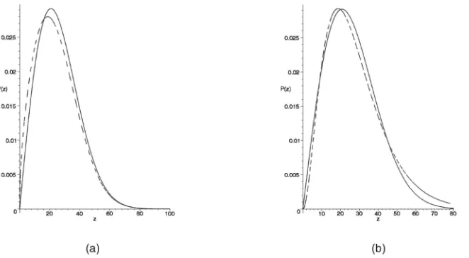
where K_¼1:06 is a normalization constant. This approx-imation is valid forz20. For the purposes of illustration, in Fig. 1a, we show the Rayleigh-Bessel distribution (7) for

_¼8and_¼20together with its approximation from (9). To measure the similarity between the two distributions

fðzÞandgðzÞ, we use the Kolmogorov-Smirnov distance:

D_¼ max 0<v<1

Z v 0

f_ðz_Þdz_ÿ Z v

0

g_ðz_Þdz

: _ð10_Þ

The Kolmogorov-Smirnov distance between the Rayleigh-Bessel distribution and its approximation is D_¼0:055, which indicates that they are statistically very similar.

The Rayleigh distribution, which is a particular case of the distribution appearing in (7) when_¼0, has been used for modeling radar returns from natural terrain in SAR images [31], [32]. Other studies assume that, after averaging a set of SAR images representing the same scene, the resulting image statistics follow a Gamma distribution [15], [28], [29], [30]. The Gamma distribution is given by:

h_ðz_{Þ ¼} z

Lÿ1

ÿ_ðLÞmLexp ÿ

z m

; _ð11_Þ

whereLandm are the parameters of the distribution and

ÿ_ðLÞis the Gamma function of orderL. We have found that we can obtain a good similarity between the Rayleigh-Bessel and Gamma distributions, appearing in (7) and (11), for a specific set of parameters. The modes of the Rayleigh-Bessel and Gamma distributions coincide when:

m_¼ 1 L_ÿ1

2þ

ffiffiffiffiffiffiffiffiffiffiffiffiffiffiffiffiffiffi 2_þ22 p

2 !

ð12_Þ

and

L¼m0:38: ð13_Þ

In Fig. 1b, we plot the Rayleigh-Bessel distribution function (7) when its parameters take on the values¼8and¼20. We show the corresponding Gamma distribution with the parameters defined by (12) and (13) in the same figure. The Kolmogorov-Smirnov distance for these two distributions is

D¼0:0414, which demonstrates the equivalence of the two models when their parameters fulfill (12) and (13).

3.2 Estimating the Parameters of the Rayleigh-Bessel Distribution

In order to use the Rayleigh-Bessel distribution as an image-model for Synthetic Aperture Radar images, we need a means of estimating its parameters. Here, we use the mode of the distribution as a route to parameter estimation. The mode of the distribution represents the most likely value [48] and it can be used as a local brightness estimate. The two

characteristic parameters of the Rayleigh-Bessel distribution (7) are the variance 2_{, which gauges the spread in the}

received radar signal, and the parameter, which measures the degree of signal interference. The location of the mode corresponds to the position where the first derivative of the probability density function from (9) is zero:

dfRBðzÞ

dz ¼0)^¼ 2þ

ffiffiffiffiffiffiffiffiffiffiffiffiffiffiffiffiffiffi 2_þ22 p

2 ¼

2 þ

ffiffiffiffiffiffiffiffiffiffiffiffiffi 2_þ2 p

; ð14_Þ

where we denote the estimate of the mode by ^ and the ratio_¼.

From Fig. 1, it is clear that the Rayleigh-Bessel is a long tail distribution and, hence, the use of robust statistics is the best route to reliable parameter estimation [39], [40], [51]. To this end, we estimate the mode and the absolute deviation using the median and the median of the absolute deviation from the median (MAD) [39], [41] estimators:

^

_¼Med_fx1; x2;. . .; xnng ð15Þ

^

_¼Medfjx1ÿ^j;. . .;jxnnÿ^jg

0:6745 ; ð16Þ

where n represents the window size used for parameter estimation. The interference parameter can be derived from (14):

^ _¼2^

2_ÿ^2

2^ : ð17Þ

The mode of the Rayleigh distribution has the property that

¼. If we consider the Rayleigh distribution as an extreme case of the Rayleigh-Bessel distribution, we find that (9) and (14) hold when:

>0:5: ð18_Þ

Next, we assess different estimators for the mode of the Rayleigh-Bessel distribution. The expected value of the meanEMean½^Šis given by:

EMean½^Š ¼

Z 1

ÿ1

zfRBðzÞdz; ð19Þ

where fRBðzÞ is the Rayleigh-Bessel distribution appearing

in (7). The expected value of the medianEMed½^Šis located at

the position where the probability density function is divided into two equally sized areas [39]. As a result:

Z EMed½^Š

ÿ1

fRBðzÞdz¼

Z 1

EMed½^Š

fRBðzÞdz: ð20Þ

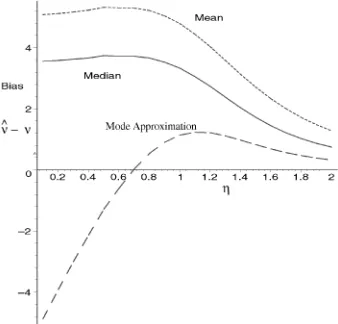
Considering the case _¼20, for various ratios in the intervalð0:05;2_Þ, we evaluate the expected values provided by the three estimators from (14), (19), and (20). The bias represents the difference between the expected value and the ground-truth parameter. The bias for each estimator is displayed in Fig. 2. As expected, we observe that the median estimator provides a smaller bias than the mean estimator. It is clear from Fig. 2 that, when using (14), we can obtain a small bias for >0:5.

3.3 The Radar Reflectivity Function

Most of the work reported in the literature on shape-from-shading relies on a Lambertian reflectance model. For synthetic aperture radar images, however, Lambert’s law

does not provide a good model of the reflectance function. The nature of interaction between the radar beam and the terrain surface is completely different from that between light and matte objects. The variation due to the physics of radiation-material interaction, the type of terrain, the presence of vegetation or man-made objects, the level of humidity, the radar beam wavelength and polarization, and the process of SAR image acquisition each affects the radar reflectivity function [2], [3], [8], [10]. To overcome this problem, in this paper, we preprocess the raw radar data by performing Lambertian correction, circumventing the difficulties de-scribed above. In this section, we turn our attention to the estimation of an empirical radar reflectance function, which can be used for the purposes of transforming the radar data into a form to which we can apply a conventional Lambertian shape-from-shading process.

3.3.1 The Lambertian Model

Shape from shading aims to recover local surface orientation from the variation in image intensity [12], [19], [20], [27]. Usually, the surface under study is assumed to be matte and to exhibit Lambertian reflectance [18], [19]. Under this restric-tion, the observed intensity is proportional to the cosine of the incidence angle, i.e., the scalar product between the unit vectors in the directions of the illuminant and the surface normal:

I_ðr; a_{Þ ¼}cos_¼NTL; _ð21_Þ

where the image intensityI_ðr; a_Þis normalized to fall within the interval ½0;1_Š. The unit vector in the surface normal direction at the locationðr; a; h_Þis given by

N_¼ ffiffiffiffiffiffiffiffiffiffiffiffiffiffiffiffiffiffiffiffiffiffiffi1 1_þp2_þq2

p ðÿp;ÿq;1Þ

T_;

ð22_Þ

wherep_¼@h

@a andq¼@h@r are the components of the surface

gradient in the r (range) and a (azimuth) directions. The unit vector in the surface normal direction is given by

whereis the azimuthal angle andis the inclination angle with the plane defined by the optic axis and the azimuthal direction, i.e., theðh; a_Þplane. With these ingredients,

cos_¼cosÿpcosffiffiffiffiffiffiffiffiffiffiffiffiffiffiffiffiffiffiffiffiffiffiffisinÿqsinsin 1_þp2_þq2

p : ð24Þ

3.3.2 SAR Reflectivity Function

As noted above, due to their physics of formation, SAR images do not exhibit Lambertian reflectance properties [11], [27]. One of our aims in this paper is to apply a correction process to the measured radar reflectance function so that conventional Lambertian shape-from-shading methods can be applied to SAR images. In this section, we consider how to perform this reflectivity transformation.

Provided that the radar illumination is directed along the range direction ( ¼0), then the reflectivity equation for SAR images is:

cos¼ R cosffiffiffiffiffiffiffiffiffiffiffiffiffiffiffiffiffiffiffiffiffiffiffiÿpsin 1_þp2_þq2 p

!

; ð25_Þ

where_Ris the reflectivity function, which is unknown for the nonLambertian case. We can make an empirical estimate ofR provided that we have at hand a digital elevation map (DEM) with ground truth height information for a given SAR image. Let us suppose that the DEM and SAR images are aligned so that pixel correspondences are known. For the SAR image, we can estimatecosfrom the normalized intensityI_ðr; a_Þ. On the other hand, the DEM image provides us with estimates of the componentsp andq of the surface height gradient. By choosing a suitable empirical parametric function, we can model the correspondence between the two data sets.

3.3.3 Empirical Derivation of the Reflectivity Function

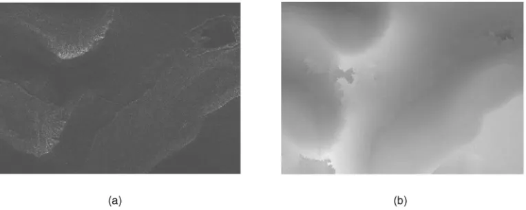
To illustrate the method outlined in the previous section, we turn our attention to the SAR image shown in Fig. 3a, which was collected over a mountainous region in Wales. The size of this image is1;8501;320pixels and corresponds to C-band (5.7 GHz) radar with a bandwidth of 90MHz and a peak power of 9.4 W, taken at an antenna depression angle_¼20

degrees. The resolution of the image is at 1.905m in azimuth and 1.499m in range. The main point to note is that the terrain features are not clear in this image due to the nonlinear characteristics of the reflectance function. Its corresponding DEM is shown in Fig. 3b and has a size of462330. The

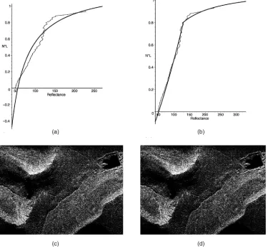
sampling in this image is, therefore, 7.62m in azimuth by 5.996m in range. The depth provided in this DEM was obtained by phase unwrapping in interferometric SAR imaging, given two SAR images taken with a stereo antenna system [52]. Several artifacts due to the radar image acquisition process can be observed in this DEM image. For the purposes of modeling the reflectivity function, we calculate the gradient for each pixel of the DEM image and its corresponding normal orientation angle using (25), and we equate it to the median estimate from the corresponding block of pixels of the SAR image. The inverse of the reflectivity function is represented with a dashed curve in Figs. 4a and 4b. The shape of this reflectivity function is characteristic of SAR images [2], [3]. We have tested two empirical models for the inverse of the reflectivity function. The first is a single continuous function over the entire domain:

Rÿ1

ðI_ðr; a_{ÞÞ ¼}Iðr; aÞ ÿ55

0:8I_ðr; a_Þ: ð26Þ

This model is shown in Fig. 4a, with a continuous line. The second model, shown in Fig. 4b, consists of a piecewise polynomial approximation, where the first branch is modeled by a polynomial of fourth order and the second branch by a polynomial of second order. The transformations of the original SAR image from Fig. 3a obtained using the inverse reflectance functions plotted in Figs. 4a and 4b, are shown in Figs. 4c and 4d, respectively. Despite the fact that the piecewise polynomial approximation is more accurate in modeling the inverse of the reflectance curve, there is no great difference in the quality of the transformed SAR images from Figs. 4c and 4d. Due to its simplicity and continuity over the entire domain of interest, we choose to use the reflectivity function, whose inverse is provided in (26), as the empirical reflectance model.

4

F

S

T

F

SAR I

In Section 2, shape-from-shading was posed as maximum a posteriori (MAP) estimation. In order to maximize the probability PðV;EjI2DÞ, we need to maximize each of its

components from (2). In this section, we model the edge-map probabilityP_ðEjI2DÞ, appearing on the righthand side

of (2). In SAR images of terrain, edges can be associated with terrain features such as ridges and ravines, but also with changes in radar image albedo or other changes in

local statistics. The existence of isolated terrain features which are limited in size is unlikely. In order to avoid edge discontinuities, we use a Markov Random Field (MRF) model [53] which enforces connectivity among the detected edge segments. The edge-map probability is computed using the approach adopted by Hancock and Kittler [54]:

P_ðEjI2DÞ ¼

Y

j

P_ðEjjI2DÞ

P_ðEjÞ

P_ðEjjEi2 NjÞ

; _ð27_Þ

where j denotes a component edge, PðEjjI2DÞ is the

a posteriori probability of the jth edge segment,P_ðEjjEi 2

NjÞ is the probability of connecting an edge segment Ej

with another edge segment Ei from its neighborhood, and

P_ðEjÞ is the a priori probability of an edge segment.

According to this approach, the edge map probability consists of two terms. The first term is a product over edge segment detection probabilities. The second term is the prior for the neighborhood edge configuration.

The maximization of the edge probabilityP_ðEjjI2DÞcan be

accomplished using a maximum likelihood edge detector. The maximum likelihood process requires the estimation of the underlying image distribution. Several algorithms have been proposed for edge detection in SAR images. In [28], [55], a Ratio-of-Averages edge detector was used for speckle images. This edge detector was shown to be optimal when the SAR image follows a Gamma distribution [29]. In this paper,

we model SAR terrain images using a Rayleigh-Bessel distribution (7). Furthermore, as shown in Section 3.1, this distribution can be replaced by the approximation in (9). We pose edge detection as a hypothesis testing problem [29], [56]. As described in [29], the maximum log-likelihood ratio j

between two neighboring regions from a SAR image, denoted byjandj_þ1, is:

j¼ jln½pðzjI2D;jފ ÿln½pðzjI2D;jþ1ފj; ð28Þ

wherepðzjI2D;jÞis the approximation in the Rayleigh-Bessel

distribution appearing in (9) and corresponding to the region j from the image I2D. The parameters of the

Rayleigh-Bessel distribution are estimated using the method outlined in Section 3.2. The probabilityPðEjjI2DÞfrom (27) is

maximized when the likelihood ratiojis maximized. This

situation corresponds to a discontinuity in the image statistics. If the probabilities of the two regions are equal, then no salient features are present andj¼0. Let us consider

the regionjto be characterized by the parameters (1; 1) and

to contain k pixels. Similarly, the region jþ1 has the parameters (2; 2) and containsn2ÿkpixels. Here,nis the

size of the window used for edge detection, which contains the regionsjandj_þ1. The probability distribution for the observed SAR amplitude in thejthregion is given by:

p_ðz_jI2D;jÞ ¼

Yk

i¼1 1 1

ffiffiffiffiffiffiffiffiffiffi Ii

21 s

exp _ÿðIiÿ1Þ 2

22 1 " #

; _ð29_Þ

where Ii is the SAR amplitude for the pixel i. Let us

consider that the number of pixels in the two regions is equal, i.e., k_¼n2_{=2. After taking logarithms, the}

log-likelihood ratio from (28) becomes:

j¼ ln 1 ^ 1 ffiffiffiffiffiffiffiffiffiffi ^ IIj

2^1 s 0

@

1

Aÿð ^ IIjÿ^1Þ2

2^2 1

ÿln 1 ^ 2

ffiffiffiffiffiffiffiffiffiffi ^ IIjþ1 2^2 s 0

@

1

A

þðII^jþ1ÿ^2Þ

2

2^2 2 ;

ð30_Þ

whereII^jandII^jþ1are the estimates of the SAR amplitude in

the regions jth and _ðj_þ1_Þth. The maximum likelihood of the Rayleigh-Bessel function occurs at the mode of the distribution, as shown in Section 3.1. If we replace^with its maximum-likelihood estimate from (17), we obtain the following log-likelihood ratio:

j¼ ln

1

^ 1

ffiffiffiffiffiffiffiffiffiffiffiffiffiffi 1_ÿ^21

2^2 1 r 0 B B @ 1 C C Aÿ ln 1 ^ 2 ffiffiffiffiffiffiffiffiffiffiffiffiffiffi 1_ÿ ^22

2^2 2 r 0 B B @ 1 C C Aÿ ^ 2 1 8^2

1þ ^ 2

2 8^2

2

; _ð31_Þ

where^jis the estimated mode from (15) and^jis the estimate

of the absolute deviation from (16), both for thejthregion. In order to obtain reliable statistical estimates, we must use a large window sizen[55]. However, by using a large window size, we recover thick edges. To overcome this problem, we perform edge thinning by using an erosion operator [57]. Edge thinning is done in such a way that it preserves the connectivity among different edge elements while maximiz-ing the edge neighborhood probability PðEjjEi2 NjÞ. The

connectivity among separate edge segments is enforced using a two-threshold hysteresis linking scheme [54]. If the log-likelihood for a SAR region exceeds a threshold value, then that region is labeled as an edge. When the log-likelihood falls between the two thresholds, then that region is labeled as an edge only if it connects two other previously labeled edge segments. Small edge segments which do not exhibit this connectivity property are eliminated.

Ridges are the peaks of structures of convex terrain topography and are characterized by a sharp decrease in the brightness when traversed in the illuminant direction. Ravines, on the other hand, correspond to bottoms of concave terrain features and are characterized by a sharp increase in the brightness when the boundary between a back-slope and a slope is traversed in the illuminant direction. These properties are used to classify the maximum log-likelihood edges as either ridges or ravines. The median estimator has been shown to be more robust than the mean when decision making is attempted using overlapping class probability densities [41]. In our case, edge classification is performed using a decision test which compares the median estimate of the radar return from two rectangular regions, oriented in the range direction, on either side of the given edge:

tE¼

Med_fI_ðr; a_ÞjrEÿd < r < rEg

Med_fIðr; aÞjrE< r < rEþdg

; _ð32_Þ

where rE is the range coordinate of the edge anddis the

width of the region used for the topographic test, in the range direction. When the edge test statistics,tE, is above a

threshold, then we classify it as a ridge. When this condition is not met, then the edge is classified as a ravine. This type of detector will also respond to rivers, which can easily be assimilated with ravines, man-made objects, and can be influenced by changes in albedo.

5

S

-

-S

SAR I

The shape from shading problem has been cast in a maximum a posteriori framework in Section 2. In this section, we show how we can estimate the probability density p_ðVjE; I2DÞ, which represents the recovery of the

vector field of surface normals from the SAR image using the available terrain features. We can represent the vector field of surface normals by means of a Markov Random Field [53]. This model decomposes the needle-map prob-abilitypðVjE; I2DÞ using the a posteriori probability of the

local surface normal p_ðVjjEj; I2DÞ and the conditional

needle-map probabilities P_ðVjjVi2 NjÞ of the surface

normalsVj depending on their neighborhoodVi2 Nj:

p_ðVjE; I2DÞ ¼

Y

j

p_ðVjjEj; I2DÞPðVjjVi 2 NjÞ: ð33Þ

Several SFS approaches have been proposed for Lambertian objects. Horn and Brooks [19] have developed a variational framework for SFS. According to their approach, there is a soft data-closeness term, which models compliance with the image irradiance equation, and a smoothing term, which regularizes (i.e., smoothes) the recovered needle map. However, this algorithm has the tendency to oversmooth the recovered vector field. Worthington and Hancock [20] rendered the process robust by using the image irradiance equation as a hard constraint rather than a data closeness constraint. In this approach, the surface normals must always lie on the surface of a cone, with the axis pointing in the illuminant direction. The apex angle of the cone is given by:

_¼arccos_ðNTL_Þ; _ð34_Þ

where N is the surface normal and L is the illuminant orientation. In our maximum a posteriori framework, the data-closeness and smoothness terms are captured by the a posteriori probability of the local surface normals

p_ðVjjEj; I2DÞ and by the smoothness prior PðVjjVi2 NjÞ

from (33). These probabilities are modeled by means of energy functions [38]. Thus, the probability maximization task is transformed into an energy minimization problem.

5.1 Vector Field Initialization

As noted above, the amplitude of a SAR image does not follow the Lambertian reflectance model. In order to apply shape-from-shading to SAR images, we must first perform Lambertian correction by applying the inverse of the reflectance function Rÿ1

, given in (26), to the raw radar data. In the case of SAR images, the signal variance, 2_,

causes an uncertainty in the estimation of the brightness. In this situation, the irradiance cone defined in [20] must be replaced by a conical envelope which spans a range of apex angles, determined by the transformed radar reflectance and the radar signal variance. The range of cosines for the cone apex angle is defined to fall in the following interval:

cos_ððt_{ÞÞ 2} cos_ð^_ð0_{ÞÞ ÿ}^

4;cosð^ð0ÞÞ þ ^ 4

where ^ð0_Þ corresponds to the orientation of the initial surface normal calculated for the mode of the local SAR distribution and^is the absolute deviation estimated using (16). The conical envelope is illustrated in Fig. 5.

The parameter, estimated using (17), corresponds to the level of interference from various scattering elements. This parameter can be used for distinguishing different types of terrain. Water strongly absorbs electromagnetic energy and is characterized by the lowest range of values for the interference parameter . Since the surface of water is horizontal, the associated surface normals are parallel to thezaxis. Shadow regions correspond to back slopes and they are also characterized by low values of . The surface normals for such regions may subtend rather large angles with the illumination direction. Layover regions have a larger bright-ness and are characterized by higher values for.

In shape-from-shading, there is a bas-relief ambiguity caused by the fact that both concave and convex surfaces produce the same variation in brightness [20]. This ambiguity can be resolved using boundary constraints. As pointed out in Section 4, we use the direction of variation in brightness at edges in order to classify them as either ridges or ravines. Naturally, the ridges belong to concave surfaces, while ravines belong to convex surfaces. As a result, ravines are attractors for the surface normals. On the other hand, ridges can be seen as repelling surface normals. In order to capture these features, we model the a posteriori needle-map probability as an energy function:

p_ðVjjEj; I2DÞ’

1

ZexpfÿjR ÿ1

ðIjðr; aÞÞÿNTjLjÿjNTjEljg; ð36Þ

whereZis a normalizing constant,Elis the tangent vector to

the closest edge from the surface normalNj. The first term in

the exponential models the recovery of the needle-map from the corrected reflectivity information. The second term models the effect of constraints provided by the whereabouts of terrain features and the direction of the local surface normals. This term is modeled using the scalar product between the surface normal and the tangent vector of the nearest edge. According to the test functiontE appearing in

(32), the surface normal is directed toward a ravine and away from a ridge, as shown in Fig. 6. Ridges are associated with divergent flow patterns in the vector field of surface normals.

Ravines, on the other hand, are associated with convergent flow patterns. By means of this energy function, the maximization of the probability density p_ðVjjEj; I2DÞ leads

to a suboptimal estimate of both the cone apex angleand the azimuthal angle (the angle between the surface normal projection in the _ðr; a_Þ plane and the azimuth direction). WhentE>1:

cos_¼laÿja

kl_ÿj_k; ð37Þ wherej_{¼ ð}jr; jaÞandl¼ ðlr; laÞare the locations of the surface

normal vector and its closest edge, respectively. We can derive a similar relation forsin. FortE<1, the signs ofcos(37) and

sinare negated (corresponding to the angle_þ).

We have shown how to estimate the opening angle of the radar reflectance cone,, and the orientation angle of the surface normal projection onto the image plane, denoted by. In the case of SAR images, the azimuthal angle of the radar beam is=2, while the inclination angle with theðh; aÞplane is denoted by, as in Section 3.3. The radar reflectance cone is rotated by the angle with respect to the image plane. In rectangular coordinates, the surface normal is given by:

NT_{¼ ½}sinsin sincos cosŠ

cos 0 _ÿsin

0 1 0

sin 0 cos 2

4

3

5: ð38Þ

The components ofNare:

N_{¼ ½}Nr Na NhŠ

¼ ½sinsin cosþcossin sincos

ÿsinsin sin_þcoscos_Š:

ð39_Þ

This is the initial direction of the surface normal that maximizes the probability density function p_ðVjjEj; I2DÞ

from (36).

5.2 Vector Field Smoothing

Since shape-from-shading is an “ill-posed” problem, the probability in (36) can be simultaneously maximized by several different surface normals. Additional constraints are necessary in order to obtain a solution and resolve ambiguities. Here, we model the smoothness prior

PðVjjVi2 NjÞfrom (33) using a local clustering energy:

Fig. 5. The range of cones defining local surface normals when illuminating a 3D surface in SAR images.

PðVjjVi2 NjÞ ’

1 Zexp ÿ

X

i2Nj

ðNi;NjÞ

8 < : 9 = ;

; ð40_Þ

where ðNi;NjÞis a regularization function depending on

the surface normals from a neighborhoodNjof thejthsite

and Z is a normalizing constant. This probability is maximized when the surface normals from the same neighborhood have similar directions.

Commencing from the initial surface normal direction as derived in the previous section, we smooth the needle-map with the goal of maximizing the smoothness prior

PðVjjVi2 NjÞ. The Euclidean distance can be employed for

calculating the similarity of neighboring surface vectors [19]:

ðNi;NjÞ ¼ kNiÿNjk; ð41Þ

where k k denotes the Euclidean distance between two neighboring vectors at sites i and j. Minimization of this regularization function can be performed using adaptive local averaging, as in [19]. At iteration t_þ1, the updated surface normals are given by:

^

N

Njðtþ1Þ ¼NN^jðtÞ ÿ" NN^jðtÞ ÿ

P

i2Nj

^

N NiðtÞ

R

" #

; ð42_Þ

where"_{2 ð}0;1_Þis the updating rate andRis the number of sites from the neighborhoodNjof the sitej.

Robust statistics [39], [51] have proven to be very useful in image processing and computer vision [40] when the raw data is corrupted by impulse noise or displays a long tailed distribution due to outliers. Recently, Worthington and Hancock [20] have shown how robust functions can be used as regularizers ðNi;NjÞin order to smooth surface normal

needle maps in the presence of surface discontinuities. In this section, we take these ideas one step further by considering various robust estimators for smoothing surface normals.

The first alternative is to use the marginal median to smooth the needle-map [41]. The updated surface normal direction is given by:

^

N

Njðtþ1Þ ¼Med l2Nj f

^

N

Nlg; ð43Þ

where the median estimator is applied on each component of the surface normal vector separately.

The second robust estimator considered in this study is the vector median [42]. This estimator selects the vector which has the lowest sum of Euclidean distances to the remaining vectors from the given neighborhoodNj:

^

N

Njðtþ1Þ ¼NN^lðtÞ; l¼arg min k

X

i2Nj

kNN^kÿNN^ik; ð44Þ

wherek_{2 N}j.

Worthington and Hancock proposed several robust methods for smoothing surface normal fields [20]. Each of these algorithms has been shown to outperform the Horn and Brooks approach [19]. The best results are obtained when using a curvature consistency algorithm. The smooth-ing achieved after applysmooth-ing this algorithm is stronger in regions of uniform local topography. At the boundary between regions with different topographic or curvature class, the smoothing is less strong. The robust regularizer used for needle map smoothing in [20] is:

ðNi;NjÞ ¼s

@Nj

@x

þs

@Nj

@y

; _ð45_Þ

wheresis a robust kernel of width parameters,i2 Nj, and

the derivatives are calculated in the neighborhoodNj. The

most effective robust error kernel was found to be the Huber function [51]:

sðzÞ ¼

s_ðNjÞ

log cosh z s_ðNjÞ

: ð46_Þ

In [20], Worthington and Hancock impose curvature consistency by adapting the kernel width s_ðNjÞ using a

variation of the Koenderick and van Doorn shape index [58]. The kernel width is set equal to:

s_ðNjÞ ¼s0exp ÿ 1 R

ffiffiffiffiffiffiffiffiffiffiffiffiffiffiffiffiffiffiffiffiffiffiffiffiffiffiffiffiffiffiffiffiffiffiffiffi X

i2Nj

ðqðiÞ ÿqðjÞÞ2

q2 v u u t 0 @ 1 A 2 4 3

5; ð47Þ

where q_ði_Þ is the shape index for a site i from the neighborhood of the site j and q_¼1=8 is the average difference in shape index between the center values of adjacent curvature classes. The shape index is calculated from the Hessian of the surface and can be expressed as a function of local surface normals:

qðjÞ ¼2

arctan @Na @a þ @Nr @r ffiffiffiffiffiffiffiffiffiffiffiffiffiffiffiffiffiffiffiffiffiffiffiffiffiffiffiffiffiffiffiffiffiffiffiffiffiffiffiffiffiffiffiffi @Na @a ÿ @Nr @r

ÿ 2

þ4@Na

@r @Nr

@a

q ; ð48Þ

where the components of the normal vector are denoted as Nj¼ ½Na; Nr; NhŠT. The surface normals are updated by

performing gradient descent on the robust regularizer:

^

N

Njðtþ1Þ ¼NN^jðtÞ ÿ"

@ ðNi;NjÞ

@Nj

: _ð49_Þ

The differentiation of the regularizer function (45) is provided in [20].

After updating the surface normal directions, we back-project them onto the radar reflectance cone. The sine of the updated anglesandare:

sin_¼

ffiffiffiffiffiffiffiffiffiffiffiffiffiffiffiffiffiffiffiffiffiffiffiffiffiffiffiffiffiffiffiffiffiffiffiffiffiffiffiffiffiffiffiffiffiffiffiffiffiffiffiffiffiffiffiffiffi ^

N N2

aþ ðNN^rcosÿNN^hsinÞ2

q

sin¼NN^rcos_sinÿNN^hsin

:

ð50_Þ

5.3 3D Height Reconstruction

In the preceding sections of this paper, we have described how to recover the field of surface normals from radar data that has been subjected to Lambertian reflectivity correction. How-ever, in most terrain analysis problems, the goal is the reconstruction of the surface height function. When having two images taken by two antennas, we can use phase unwrapping for 3D surface reconstruction [52]. However, in the case analyzed in this paper, we are provided with only one image. In the previous sections, we have shown how we can estimate a field of surface normals from a single SAR image. Formally, we are interested in the problem of reconstructing a surface from a Gauss map. In this section, we describe a simple surface integration method that can be used to reconstruct surface height from local surface orientation information [43]. The suggested height estimation algorithm is iterative. At each iteration, the calculation of height is a two step process. In the first step we decide which neighboring site is appropriate to be used as reference for estimating the unknown height, while, in the second stage, we estimate its height.

We wish to estimate the surface height at the pointBwhich has site coordinatesði; jÞ. This site is a neighbor of the location

Awhich has site coordinates_ðr; a_Þand known height. Hence, ði; jÞ 2 N ðr; aÞ. Let the perpendicular to the image plane at location Bintersect the surface at location C, and let the known height of this location beHði; jÞ. Further, letkBCk represent the difference in surface height for locationsAand

Bon the image plane. Since the height atBis unknown, we must select from its set of neighbors the reference site of predetermined height from which we can make the most reliable height estimate. The selection of the reference site proceeds as follows: First, we construct the plane formed by the surface normal vector at the siteBand the perpendicular at that site, i.e.,BC. Next, we compute the distances from all the sitesði; j_{Þ 2 N ð}r; a_Þto this plane, as

dða; rÞ ¼jðaÿjÞNffiffiffiffiffiffiffiffiffiffiffiffiffiffiffiffiffiffiffiaÿ ðrÿiÞNrj N2

aþNr2

p : ð51Þ

We search for sites which minimize this distance. To do this, we set a distance thresholdf. This distance threshold is initially taken as f_¼0, i.e., we test if Ais located on the plane formed by BC and the surface normal. At every iteration, for each site from the entire lattice, we choose only those locations which fulfill the condition:

dða; rÞ f: ð52_Þ

By finding the minimum ofd_ða; r_Þfor all the sites of known height that fulfill (52) in the neighborhoodN ði; jÞ, we select the site _ðk; l_Þat which to update the height. The site is the one that satisfies the condition:

ðk; l_{Þ ¼}arg min

ða;rÞ2N ði;jÞfdða; rÞg: ð53Þ

In the case whenNa¼0, we compute the modified distance

d_ða; r_{Þ ¼}max_fja_ÿj_j;_jr_ÿi_jg; _ð54_Þ

whereði; jÞ 2 N ða; rÞ.

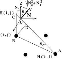
In the second stage, the heightHði; jÞis computed using simple trigonometry. The reference siteAof known height and the siteBof unknown height are shown in Fig. 7. From this figure, it is clear that we can use the similarity of two triangles to estimate the unknown height. The first triangle is formed by the surface normal vector and the h axis (which is parallel withBC) and it is denoted by UVZ. The second triangle, denoted by ABC, is formed by the sitesA

andBon the image plane and the locationCon the surface, i.e., the point at which we estimate the height. From the similarity of these triangles, we have:

kBC_k

kZV_k¼

kAB_k

kUZ_k¼

kAC_k

kUV_k; ð55Þ

Fig. 7. The evaluation of 3D height information.

wherekABkrepresents the distance between the neighbor-ing sitesAandB,kBCkdenotes the difference of height:

kBC_{k ¼ j}H_ði; j_{Þ ÿ}H_ðk; l_Þj: _ð56_Þ

After replacing the distances in (55), we get:

jH_ði; j_{Þ ÿ}H_ðk; l_Þj ffiffiffiffiffiffiffiffiffiffiffiffiffiffiffiffiffiffiffi N2

r þNa2

p ¼

ffiffiffiffiffiffiffiffiffiffiffiffiffiffiffiffiffiffiffiffiffiffiffiffiffiffiffiffiffiffiffiffiffiffiffiffiffi

ðlÿjÞ2

þ ðkÿiÞ2 q

Nh ¼

kAC_k

1 ; ð57Þ

whereHði; jÞis the height for the siteði; jÞandHðk; lÞis the known height at the reference location ðk; lÞ, chosen according to the condition in (53). From this relationship, it is clear that, when Nh!0, then Hði; jÞ ! 1. This can

lead to discontinuities in the height estimation process. In order to avoid discontinuities, we must ensure that the reconstructed surface is finite. Let us consider the projection of the location B onto the surface and let this point be denoted byD. We assume that the height_kBC_kat site_ði; j_Þ

is approximated by _kBD_k. This simplification will ensure that we avoid singularities in the case when reconstructing the surface height from the field of surface normals. In this case, using the similarity between the triangles ABD and

UV Z, we find that:

kBD_k

kZV_k¼

kAB_k

kUV_k¼

kAD_k

kUZ_k: ð58Þ

Substituting for the distances in the above equation, we obtain

jH_ði; j_{Þ ÿ}H_ðk; l_Þj ffiffiffiffiffiffiffiffiffiffiffiffiffiffiffiffiffiffiffi N2

r þNa2

p ¼

ffiffiffiffiffiffiffiffiffiffiffiffiffiffiffiffiffiffiffiffiffiffiffiffiffiffiffiffiffiffiffiffiffiffiffiffiffi

ðl_ÿj_Þ2_{þ ð}k_ÿi_Þ2 q

1 ¼

kAD_k Nh

: _ð59_Þ

As a result, the height update equation for the height corresponding to locationBis

H_ði; j_{Þ ¼}H_ðk; l_Þ m

ffiffiffiffiffiffiffiffiffiffiffiffiffiffiffiffiffiffiffiffiffiffiffiffiffiffiffiffiffiffiffiffiffiffiffiffiffi

ðl_ÿj_Þ2_{þ ð}k_ÿi_Þ2

q ffiffiffiffiffiffiffiffiffiffiffiffiffiffiffiffiffiffiffi N2

r þNa2

q

; _ð60_Þ

where the sign depends on the direction of the surface normal vectorNandmis a normalization constant which determines the vertical scale. The sign is positive if the projection of the surface normal onto the lattice plane points away from the site ðk; lÞand toward the siteði; jÞ. If this is not the case, then the sign is negative. The two signs respectively correspond to ascending and descending slopes. We calculate the height for all the locations which fulfill the condition given in (53) for a chosen distance threshold f by considering only one reference height at the time. At the next iteration, we increase the maximal distance thresholdffrom (52), thus allowing us to update the height at additional sites. The two steps of the algorithm are repeated until all sites are visited. As we progressively increasef, we will find height estimates for an increasing number of sites. The maximal value for this threshold distance isf¼1. After evaluating the heights at all sites in the image, we calculate the local surface normals from

Fig. 9. Fitting the SAR image distribution with Rayleigh and

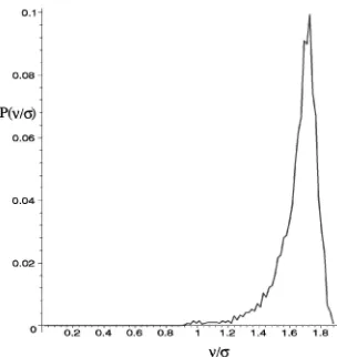
Rayleigh-Bessel models. Fig. 10. Distribution of the ratio between the mode and absolute deviation.

the local height differences onrandadirections and compare them to the surface normals from the original vector field. The heights and the surface normals are iteratively updated by passing successively through the data until we achieve their consistency. The entire shape-from-shading method for SAR images is described in the diagram from Fig. 8. The first stage consists of solving low-level image processing pro-blems such as nonlinear Lambertian correction and estimat-ing edge features from radar image statistics. The SAR image statistics and the edge features are used in a shape-from-shading framework in which we model fields of surface normals. Eventually, the surface normals are used for calculating the 3D height information finalizing the mapping of a single SAR image of terrain into its corresponding 3D topography.

6

E

R

We have applied the proposed algorithm for radar shape-from-shading to SAR images of mountainous terrain captured from an aircraft. Fig. 3a shows a representative SAR image. Fig. 9 shows the amplitude distribution for a100100pixel region selected from this image. Superimposed on the image data distribution are the estimated Rayleigh-Bessel (7) and

Rayleigh distributions. The Kolmogorov-Smirnov distance (10) of the fitted distribution isD_¼0:0447for the Rayleigh-Bessel andD_¼0:1166for Rayleigh. We have split the image into blocks and estimated the ratio =^ ^. The resulting histogram of this ratio for the entire image is shown in Fig. 10. The Rayleigh distribution has the property that=¼1. However, only a small percentage of data is located around this value, as we can see in Fig. 10. These results suggest that the Rayleigh-Bessel distribution is more appropriate than the Rayleigh distribution for SAR images of terrain.

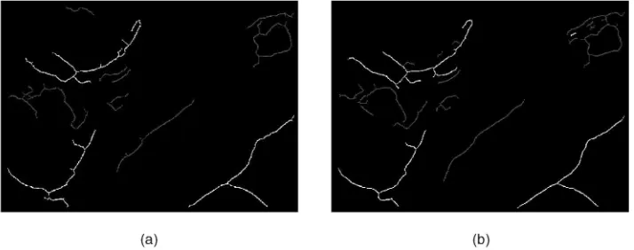
In order to recover terrain shape from the given SAR image, we apply the maximum a posteriori model described in Section 2. First, we estimate the probability density function corresponding to edges, provided in (27). We detect the edges using the algorithm described in Section 4. The gradient image obtained when using the optimal estimator for the Rayleigh-Bessel distribution (31) is shown in Fig. 11a. For comparison, Fig. 11b shows the gradient when the ratio-of-averages algorithm is used instead [28], [29]. In both cases, we have used a3131pixel window. The gradients obtained with the optimal edge detector for the Rayleigh-Bessel distribution are sharper and clearer than those detected by the ratio-of-averages estimator. The edges labeled as ridges and ravines using the classifier defined in (32) are shown in Fig. 12a. Fig. 12b displays the corresponding result obtained with the ratio-of-averages edge detector. The ridges are shown in a lighter gray-level, while the ravines are in a darker gray-level. From these figures, we can identify the main terrain features of the SAR image from Fig. 3a.

After applying the inverse reflectivity function derived in Section 3.3 and plotted in Fig. 4a, we obtain the image from Fig. 4c. We segment this image into blocks of size

2020 and we estimate the parameters of the Rayleigh-Bessel distribution (7). The interference parameter denoted by is used to identify the regions covered by water and the back-slopes of mountains. We compute the apex angle of the reflection cone using the locally estimated mode of the Rayleigh-Bessel distribution. The edge map represented in Fig. 12a is used as a constraint in the recovery of the vector field of surface normals. The maximization of the local a posteriori surface normal probabilities p_ðVjjEj; I2DÞ

as described in Section 5.1, provides the vector field shown in Fig. 14a. From this needle map, it is clear that the ravines and ridges are estimated as centers of convergent and divergent vector fields of surface normals.

Fig. 12. Edge classification in a SAR image. (a) Edge classification when employing the optimal edge detector for the Rayleigh-Bessel distribution. (b) Edge classification when employing the ratio-of-averages edge detector.

We employ the iterative algorithm described in Section 5.2, for smoothing the vector field. This iterative updating involves two stages. In the first stage, each vector normal is modified toward an estimate of its neighbor vectors while maintaining the constraints imposed by the image statistics and by the reflectance function (36). In the second stage, the consistency of the updated surface normal with the local variance is verified according to (35). If a vector has its corresponding cone apex angle located outside the range provided by the local SAR image statistics, its value is corrected accordingly. The iterative updating algorithm of the surface normals continues until convergence is achieved.

The vector field obtained after averaging according to (42) is shown in Fig. 14c, while the vector fields smoothed by employing the marginal median (43) and the vector median

(44) estimators are shown in Figs. 14d and 14e, respectively. Fig. 14f shows the result obtained when using the surface curvature consistency algorithm (45)-(49). For each case, the smoothing neighborhood is a matrix of33vectors (R¼9). It is clear from all these figures that the resulting vector fields are quite smooth. The vector field of surface normals corresponding to the digital elevation map represented in Fig. 3b is shown in Fig. 14b. For quantitative comparisons, we use this vector field as a reference. This vector field is not very smooth due to the inaccuracies in the phase unwrapping recovery employed for calculating the DEM image. We consider two error measures in order to estimate the accuracy of the proposed algorithms. The first one is the mean square error between the reference vector field, denoted asN, and that of the smoothed vector field,NN^, and is given by:

MSE_¼ 1 MP

XM

x¼1 XP

y¼1

kN_ðx;yÞÿNN^ðx;yÞk; ð61Þ

whereN_ðx;yÞdenotes the vector located at the siteðx; yÞ. The

second error measure is the average cosine between the two vector fields:

MCE_¼ 1 MP

XM

x¼1 XP

y¼1

N_ðx;yÞNN^ðx;yÞ: ð62Þ

For the initial vector field of surface normals before applying any smoothing, we obtainMSE_¼0:873andMCE_¼0:606

when considering as reference the vector field of the DEM. The convergence of surface field smoothing algorithms with respect to MSE is shown in Fig. 13.

Finally, we present some results to illustrate the surface reconstructions that can be obtained from smoothed needle-maps delivered by our shape-from-shading method. In Figs. 15 and 16, we compare the reconstructed surfaces with the ground truth provided by the digital elevation map. In the digital elevation map shown in Fig. 15a, there are a number of clear topographic features. First, there is a semicircular ridge in the top lefthand corner. Midway along the ridge, there is a rill which descends and meets with a ridge just below the main peak. There is also a deep valley which cuts across the plot at about 45 degrees and ends in the top righthand corner. The reconstructed maps are scaled to fit the range of heights for the DEM. In Fig. 15b, we show the surface reconstructed from the initial needle-map directions as they are derived from the statistics of the SAR image. Here, the valley emerges clearly, but the semicircular ridge and the rill are not well-defined. In

Figs. 15c and 15d, we show the surfaces obtained from the needle-maps delivered by marginal median smoothing and vector median smoothing. In both cases, the semicircular ridge and the rill are reconstructed. However, in the case of vector-median smoothing, the valley structure is badly disturbed. In Fig. 16, we provide a comparison with the results obtained with alternative algorithms. Fig. 16a shows the result obtained with the robust smoothing method of Worthington and Hancock [20]. Here, the semicircular ridge and the valley emerge well, but the rill is not detected. When vector averaging is applied to the initial needle-map, then the valley is well located, but the other features are oversmoothed, as can be seen in Fig. 16b. In Figs. 16c and 16d, we respectively compare with the Bichsel and Pentland [44] and Zheng and Chellappa algorithms [27]. These two algorithms compared favorably with other shape-from-shading algorithms in the survey from [23]. In order to use these SFS algorithms, we have processed the SAR image as in [11]. The Bichsel and Pentland method locates the semi-circular ridge, but exaggerates its height and introduces a large number of noisy peaks in the proximity of the valley. Some of the topographic features are just discernible in the output of the Zhang and Chellappa algorithm and the height is underestimated.

In Table 1, we provide numerical results for MSE and MCE for the surface normal fields, the average height error in the 3D surface reconstruction, as well as the number of iterations needed for convergence when smoothing the vector field of surface normals. From this table, we can see that the robust algorithms perform better than the classical approach of local vector averaging of the surface normals. Also, the number of iterations is much lower for the robust estimators. If the

estimated and ground truth reference surface normals have the same orientation, then the cosine of their angle difference would be 1. For comparison, we consider the algorithms of Bichsel and Pentland [44] and Zheng and Chellappa [27].

In Fig. 17, we show results obtained for radar images of Ayers Rock (mountain Uluru) and a neighboring region of mountainous topography. In Figs. 17a and 17b, we show the SAR images. Figs. 17c and 17d display the smoothed needle maps, while Figs. 17e and 17f show the reconstructed surface height data. In the case of the image from Fig. 17a, which shows Ayers Rock, the lower lefthand edge of the structure is well-reconstructed in both the needle-map and the height data. While the conditions of SAR image acquisition may be different for these images, we have considered the same reflectivity function as that modeled by (26). Unfortunately, the shading process fails in the shadow regions in the upper part of the image. Significant regions of shadowing or layover can pose problems to the proposed technique. In the case of the image from Fig. 17b, which shows a series of ridges, the overall structure is detected, but the fine detail is not reconstructed well.

7

C

This paper proposes a new approach for terrain reconstruc-tion from SAR images using shape-from-shading. We embed the SFS approach in a maximum a posteriori framework. The novelty of the proposed approach consists of the way that various techniques are combined in order to solve the problems posed by terrain reconstruction from SAR images.

The main components of the proposed probabilistic model are: 1) the irradiance equation, 2) surface smoothing, and 3) the edge map topography constraint. We showed that the

Fig. 16. Reconstructed 3D surfaces from the SAR image: (a) Using surface consistency smoothing for surface normals, (b) using averaging of surface normals, (c) surface generated using Bichesel and Pentland shape-from-shading, and (d) surface generated using Zheng and Chellappa shape from shading reconstruction algorithm.

TABLE 1