Bayesian estimation of genomic copy number with single nucleotide polymorphism genotyping arrays

R E S E A R C H A R T I C L E

Open Access

Bayesian estimation of genomic copy number

with single nucleotide polymorphism

genotyping arrays

Beibei Guo

, Alejandro Villagran

, Marina Vannucci

, Jian Wang

, Caleb Davis

, Tsz-Kwong Man

,

Ching Lau

, Rudy Guerra

Abstract

Background:The identification of copy number aberration in the human genome is an important area in cancer research. We develop a model for determining genomic copy numbers using high-density single nucleotide polymorphism genotyping microarrays. The method is based on a Bayesian spatial normal mixture model with an unknown number of components corresponding to true copy numbers. A reversible jump Markov chain Monte Carlo algorithm is used to implement the model and perform posterior inference.

Results:The performance of the algorithm is examined on both simulated and real cancer data, and it is compared with the popular CNAG algorithm for copy number detection.

Conclusions:We demonstrate that our Bayesian mixture model performs at least as well as the hidden Markov model based CNAG algorithm and in certain cases does better. One of the added advantages of our method is the flexibility of modeling normal cell contamination in tumor samples.

Background

Gene dosage variations occur in many diseases, as well as in normal populations (e.g., [1,2]). In cancer, copy number losses and gains are known to contribute to alterations in the expression of tumour-suppressor genes and oncogenes, respectively, see for example [3,4]. Developmental abnormalities, such as Down, Prader Willi, Angelman and Cri du Chat syndromes, result from gain or loss of one copy of a chromosome or chro-mosomal region. Thus, detection and mapping of copy number abnormalities provide an approach for associat-ing aberrations with disease phenotype and for identify-ing critical disease-causidentify-ing genes. As an example, Rendon et al. [5] constructed a first-generation copy number variation (CNV) map of the human genome through the study of 270 HAPMAP individuals from four populations with ancestry in Europe, Africa or Asia, [6]. A total of 1, 447 copy number variable regions (CNVRs), covering 360 megabases (i.e., 12% of the

genome), were identified in this study. These CNVRs contained genes, disease loci, functional elements and segmental duplications.

DNA from the individuals in the study of [5] was ana-lyzed for CNV using two technologies: single-nucleotide polymorphism (SNP) genotyping arrays, and compara-tive genomic hybridization (CGH). Array-based Comparative Genomic Hybridization (aCGH) is a mole-cular-cytogenetic method for the analysis of DNA copy number changes [1]. The method is based on hybridiza-tion of fluorescently labeled tumor DNA and reference DNA on a microarray platform containing Bacterial Artificial Chromosome (BAC) clones or spotted DNA. As a gold standard, it is robust in identifying long seg-ments of chromosomal alterations. However, although the resolution of aCGH has been improved, it is still not high enough to detect amplifications or deletions of relatively short segments, [7] and [5]. The high-density SNP array, which can accommodate hundreds of thou-sands of SNP probe sets simultaneously, is an alternative approach to detect genome wide copy number aberra-tions which has much higher resolution than CGH, see [8]. Compared to CGH, SNP array based experiments

* Correspondence: [email protected] 1

Department of Statistics, Rice University, 6100 Main, Houston, TX 77005-1827, USA

Full list of author information is available at the end of the article

are newer and are becoming more popular for copy number analysis.

A number of statistical methods have been proposed to estimate copy numbers from various platforms. Two of the most popular methods for SNP arrays are dchip and Copy Number Anlyser for GeneChip (CNAG). Zhao et al. [9] proposed dChip, an algorithm that derives model-based estimates of SNP copy numbers that incorporate probe effects and a hidden Markov model (HMM) to infer integer-valued copy numbers. Although the current version of the dChip software can accommodate the newer SNP arrays, such as the Affy-metrix 250K array, it is not optimized for it. Nannya et al. [10] developed the CNAG algorithm, which accounts for the length and GC content of the PCR pro-ducts. Accounting for the length and content of GC ele-ments seems to improve copy number inference [10]. Another source of variation that can affect a copy num-ber analysis is the so-called “genome wave” [11,12], a genome-wide spatial autocorrelation pattern in signal intensity. Since the genome wave may be confounded with the copy number profile across a chromosome, investigators should examine their intensity data for its presence and adjust the data accordingly. Since the genomic wave [11] is thought to be in large part due to GC content, the CNAG algorithm can also be thought of as an adjustment for wave effects possibly present in SNP array data. Again, an HMM is used to infer integer copy numbers. The HMM approach can also be found in the algorithms underlying QuantiSNP [13] and PennCNV [14], both of which use the log-R-ratio and

B-allele frequency to infer the copy number state of each SNP. These two methods consider a six-state Mar-kov model which distinguishes copy-neutral loss of het-erozygosity from the normal state. Most HMM based algorithms use the Viterbi algorithm [15] to infer integer copy numbers.

To date, there are a handful of Bayesian methods for copy number inference. Most are for CGH data, but a few exist for SNP data. Rueda and Diaz-Uriarte [16] proposed RJaCGH, a nonhomogeneous HMM in a Baye-sian context for CGH data. Instead of prespecifying the number of states as a conventional HMM, a reversible jump Markov Chain Monte Carlo (MCMC) method is used to allow for varying numbers of hidden states. Bayesian model averaging is used to obtain final esti-mates. Pique-Regi et al. [17] developed a method called Genome Alteration Detection Algorithm (GADA) that is based on sparse Bayesian learning [18]. The approach takes advantage of the a priori assumption that the number of copy number alterations (break points) is sparse with respect to the number of probes. As with several other methods, advantage is also taken of the fact that the copy number pattern across a chromosome

can be modeled as a piecewise constant function or vec-tor. The GADA output gives copy number results in the form of a segmentation, viz., a collection of ordered seg-ments defined by their breakpoints and amplitudes. To obtain integer-valued copy numbers or alteration status (loss, normal, gain), the estimated segments must be analyzed by a thresholding procedure, such as Huang et al. [19]. GADA can be applied to both CGH and SNP based data. Rancoita et al. [20] also make use of piece-wise constant modeling in their algorithm, mBPCR, which is a modification of the original Bayesian Piece-wise Constant Regression (BPCR) method developed by Hutter [21]. This method is general for data that take the form of a piecewise constant function with unknown segment numbers, boundaries, and levels. Rancoita et al. illustrate the mBPCR method using SNP data, but it appears that log-ratios based on CGH data can also be analyzed.

In addition to those described above, several other sta-tistical methods have been developed for copy number analysis. They vary in their assumptions, inference (seg-mentation, alteration status, integer copy number), plat-form (CGH, SNP), input data (e.g., CEL files or generic normalized log-ratio), and software implementation (e.g., commercial, web-based, customized academic program). Winchester et al. [22] describe and compare a number of methods. No method stands out as uniformly best and Winchester et al. suggest analyzing copy number data with at least two different methods to assess con-sistency and robustness of results. In this paper, we could not consider many of those methods for perfor-mance comparison because most of these algorithms do not estimate integer copy numbers.

Most of the copy number methods assume normalized log-ratios as input. Relatively few include adjustments for known factors affecting inference. GC content and fragment length have been mentioned as factors affect-ing copy number inference. Another factor from tumor samples is normal cell contamination. Indeed, most tumor samples are heterogeneous and include both can-cer cells (with copy number aberrations) and normal cells. The larger percentage of normal cells present, the more difficult it is to infer copy number aberrations in the tumor cells; the log-ratios tend to shrink to the null value of zero. None of the above methods implement an adjustment for normal cell contamination. Below we show how our proposed method can account for this factor.

segments (e.g. BACs). Spatial correlation was induced through the weights of the mixture via Markov random fields. In our approach, instead of considering three states, we allow for an unknown number of mixture components and achieve inference using a reversible jump Markov chain Monte Carlo method. As in [23] we use Markov random fields to account for correlated neighboring SNPs. In contrast to models that incorporate HMMs to infer integer copy numbers, our modeling approach uses infor-mation (neighboring SNPs) on both sides of a SNP. In addition, we account for cell contamination by shrinking the theoretical copy number log-ratios towards zero. The implementation only requires ordered (normalized) log-ratios and, therefore, may be applied to data from any plat-form suitable for copy number estimation. In Section 2 we present the model and method of inference. Section 3 reports on a simulation study and application to real data. The real data study includes cases where cytogenetics has shown large regions of gain or loss and we also show novel smaller regions detected by our algorithm. The new aberrations are validated by CGH and/or PCR. A discus-sion is given in Section 4 and an Appendix provides details on the MCMC algorithm.

Methods

Model

Let yi be the preprocessed log-ratio of SNP i ordered along the chromosome. Following the notation of [24], we consider a normal mixture model withkunknown components corresponding tokcopy numbers,

p yi k ijN y j

k

i j j ( | , , ,ZZ PP VV2) ( | , )

1

2

= =

∑

where μ= (μ1,...,μk) and VV2=(V₁2,…,V_k2) represent the vectors of means and variances of thekcomponents. The matrix of weightsω= (ωij) is such that 0≤ ωij≤ 1

and Z_ij j k

= =

∑

1 for all i. In our application the

com-ponents represent the true copy numbers (i.e. copy number equals to 0, 1, 2, 3,...). Given a chromosome withnSNPs, letz1,...znbe the allocation variables, indi-cating to which mixture component SNPi belongs to. These are marginally distributed according to a multino-mial distribution with

p z( i= j k| , , ,ZZ PP VV2)=Zij, (2) forj = 1,...,k. Since copy number aberrations tend to occur over contiguous segments, we impose that neigh-boring SNPs have similar multinomial probabilities of belonging to the copy number classes. To this end, fork

components we introduce k independent Gaussian Markov random fields (GMRF), xj = (xij,i = 1,...,n), see [24] and [23], each with joint distribution

p h c h

exp h x x x

j

ij i j i i

ij i

n

( )

{ ( ( ) )}

|

~

x =

( )

− − ′ +

′ =

∑

∑

1 2

2 2 1

(3)

whereΣi~i’denotes the sum over all pairs of neighbors

and where _{c h} n _hg

i i

n

( )

( )

∏

(

)

1

1 2

π , withg1,...,gn the eigenvalues of a matrix of coding adjacencies. Since the conditional distribution ofxijonly depends on its neigh-bors, neighboringxij’s will tend to have similar values. The parameterhis non-negative and controls this effect: large values ofhinduce smoother realizations in the GMRF, and ash® 0 independent realizations take place. For the weights,ωij’s, we borrow spatial correlation from the GMRF’s by defining logistic transformations of the type

Z I

I ij

ij

il l

k exp x

exp x

j k

=

(

)

=

∑

( )

, , , ,

1

1 ₍₄₎

wherejis a scaling factor specified by the user. In the simulation study of Section 3 we investigate robustness of the results to different valuesjof and varying num-ber of neighbors.

Prior distributions

In this section we discuss the prior distributions for the model parameters, including the number kof mixture components, the normal mixture means and variances, and the smoothing parameterh.

1. Number of mixture components, k

We choose a truncated Poisson distribution with mean 2 as the prior distribution of the number of components,k,

k~TPoisson

{

}

withkmaxa pre-specified large integer. We take kmax = 7 for illustration purposes, corresponding to copy numbers 0, 1, 2, 3, 4, 5,and> 5. Here 7 is arbitrary, and we can use any positive value that makes sense for the data under consideration.

2. Normal mixture means

We deviate from the approach of [24] by constructing

kmaxuniform distributions, {νj=U(aj,bj), j= 1,...,

We choose the intervals to be non-overlapping and to contain the theoretical copy number values. According to [10], the observed mean values for the 7 compo-nents without contamination are approximately -1.24, -.49, 0, .365, .657, .899 and 1.106 for copy numbers 0, 1, 2, 3, 4, 5 and > 5, respectively. In this paper results were obtained using the following intervals: (-2, -.8), (-.6, -.25), (-.05, -.05), (.15, .4), (.45, .66), (.75, .9), (.95, 1.3), corresponding to copy numbers 0, 1, 2, 3, 4, 5, > 5, respectively. These intervals are the default values we used in the application and have worked well in most cases. Our results did not show sensitivity to the actual values we used for the extremes of the intervals, i.e., other disjoint sets of intervals worked well too.

Remark 1: Due to normal cell contamination, the true

log-ratios tend to shrink toward zero, and in practice some degree of normal cell contamination tends to be present. We thus decided to center the uniform distri-butions closer toward the null value of zero rather than at the theoretical means given above, except for CN = 0 and CN > 5. These exceptions are largely due to where we wanted to locate the respective uniform support; see Remark 3 below.

Remark 2: Moving the uniform intervals closer to

zero resulted in some of the theoretical means being located close to a uniform boundary. For example, for CN = 5, the theoretical mean of .899 is just inside the right boundary of .9. This does not cause a problem of misclassification since normal cell contamination brings the mean closer to the left boundary.

Remark 3: We also varied the length of the uniform

intervals since the log scale makes the consecutive theoretical values become increasingly closer to each other; the consecutive pairwise distances between the theoretical means from -1.24 to 1.106 are .75, .49, .365, .292, .242, .207. If the uniform intervals were forced to be of equal length we would have either relatively short non-overlapping intervals or over-lapping long intervals. Since the uniform inter-vals are not of equal length, the gaps between the intervals are unequal, as well.

In cases where the exact percentage (p) of normal cells is known then such intervals can be chosen to contain

log p j p b b

2

2 1

2

+ − +

+ ⎡

⎣⎢

⎤ ⎦⎥

( )

,

for any copy number j, with background factor b, see [10], and then choosing the length of the intervals so that thekmaxintervals are non-overlapping.

3. Normal mixture variances

We assign an inverse gamma prior distribution to

σ2j. In the application we center this distribution on

0.2 and induce a vague specification by letting the variance be large.

4. Smoothing parameter

We assign h a uniform distribution with a wide range, h ~ U (0, hmax), with hmax = 1000, 000, to induce smooth realizations.

We provide further discussion of these prior selec-tions below in Section 3 in the context of the simu-lations and real data applications.

Posterior inference

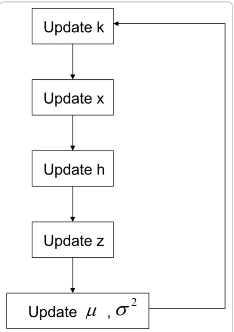
We employ MCMC with reversible jump to achieve pos-terior inference. A flowchart of our MCMC algorithm for posterior inference is given in Figure 1. We note that while updates on x and z are done at each SNP locationi, the updating steps onk,h, μands2are glo-bal, i.e., done at chromosome level. Steps are described

Update k

Update x

Update h

Update z

Update ,

P

V

2

Figure 1 Flowchart of the MCMC algorithm for posterior inference. Updating steps onk,μands2_{are done at the}

below in their corresponding order in the implemented algorithm. Additional details are given in the Appendix.

• Updatingk: This step causes creation or deletion of components, therefore requiring the sampler to jump between subspaces with different dimensions. To implement the sampler, we use reversible jump MCMC (RJMCMC), see [25] and [26]. We updatek’=

k+ 1 with probabilitybk, andk’=k- 1 with probability

1−b b_{k 1}=1b_k =0b_k= 5 k= …2 k_max−1

max

( , , . for , , )_{. Ifk}’_=k+

1, we draw a new component from the remainingkmax

- kcomponents with equal probability, and drawμ*

from the corresponding uniform distribution. We also draw V_*2 _andx

*from the prior distributions. We then

increase the dimensions of the vector parametersμ’= (μ,μ*), VV2′=(VV2,V_*2), andx’= (x,x*) and accept the

new component with probability:

min

b

k p k b

k kp k N y k k ij j k i max 1 1 1 1 1 1 1 1 1 , ( ) ( ) ( ) ( − + + − ⎛ ⎝ ⎜ ⎜ ⎜ ⎜ × ′ + = +

∑

( | , ) ′ ′ ⎞ ⎠ ⎟ ⎟ ⎟⎟ = =

∑

∏

k

i j

i n

ijN y j

2

1

2 1

(6)

If k’=k- 1, we instead randomly pick a component from the discrete uniform distribution on {1,...,k} and remove P V_*, _*2,x_* from μ, s2, x. Similarly, the acceptance probability is

min b

k k p k

b kp k N k k ij j k max 1 1 1 1 1 1 1 1 1 , ( ) ( ) ( ) ( ) ( − = − − − − − ⎛ ⎝ ⎜ ⎜ ⎜ ⎜ ×

∑

j k i j i n ij j | , ( | , ) ) ′ ′ ⎞ ⎠ ⎟ ⎟ ⎟⎟ = =

∑

∏

1

2 1

(7)

• Updating x: We update each location using a

Metropolis-Hastings step, see [27] and [28]. We per-form these n updates sequentially, i.e., we update (x11,...,x1k) first, then update (x21,...,x2k), etc.. For each locationi, we use a proposal distribution of the type

N x h x hn hn ij i j i i i i j k ′ + ⎛ ⎝ ⎜ ⎜⎜ ⎞ ⎠ ⎟ ⎟⎟ ′ ′ =

∑

∏

where ni is the number of neighbors at locationi. The acceptance probability is

min N y N y ij j ij j j k i j j k i j 1 1 2 1 2 , ( | , ) ( | , ) ′ ⎛ ⎝ ⎜ ⎜ ⎜⎜ ⎞ ⎠ ⎟ ⎟ ⎟⎟ = =

∑

∑

Z P V

Z P V

whereω’are the weights associated to the proposedx.

• Updatingh: We use a Metropolis-Hastings

ran-dom walk with a proposal defined by a truncated

normal distribution, h′~TN h( ,V_h2) (I0_{≤ ′ ≤}h h_max). In applications we chose sh to have acceptance ratios between 40% and 70%.

• Updating allocations: Using a Gibbs step, we

draw thenallocations independently from

p z j k h

N y I j k

i

ij i j j

( | , , , , , , )

( | , ) [ , ].

=

∝ ∈

{

}

y PP VV2 x

2

1

I P V

Z (8)

•Updatingμ, s2,:For eachj, we consider thekmax intervals and select that one with largest posterior probability, then sampleμjfrom a normal distribu-tion truncated at this interval. In the iteradistribu-tions it may happen that two or more P′js are sampled to the same interval. In this case, we combine these components and updatek. The newμj, sj,xj, for the new formed component are taken to be the weighted sum of the original ones by the sample size. We then redefinezand calculateω. We draw σ2_j from its full conditional. See Appendix for the forms of the full conditionals.

For posterior inference, the primary parameters of inter-est are the weightsω’s. We propose an allocation rule as follows: at each iteration we record the probability of each SNP to belong to each of thekmaxcomponents (we assign zero if a component is empty). After the MCMC is done, we average all theω’s and assign a SNP to the component that has the largest probability. We check reproducibility of the clustering with different starting values.

Programming in some version of C and parallel comput-ing by chromosome and/or chromosome arm will likely significantly reduce the time.

Results and Discussion

Simulation Study

We first investigate the performance of our model through simulation experiments. In the next Section we compare our method with two alternative methods in the context of actual tumor samples from leukemia and ependymoma cancers.

We conducted two sets of simulations studies. The first set was designed to examine the influence of hyperpara-meters in the prior specifications: the scaling parameter,

j, of the logistic transformation for the GMRF and the number of smoothing neighbors,nb. Based on the results of the first set of experiments we then conducted a sec-ond set of experiments by setting these two parameters at fixed (default) values in order to assess performance of our algorithm. For scenarios with no contamination the log-ratios corresponding to copy numberjwere indepen-dently drawn from a normal distribution with the corre-sponding theoretical mean for copy number j and a standard deviation chosen to achieve a given SNR. For scenarios with contamination the log-ratios correspond-ing to copy numberjwere independently drawn from a normal distribution with mean log2 ( )

1 2

2

j p p b

b

− + +

+ ,

wherepis the percentage of contamination andbis the background factor, see [10].

In the first set of simulation studies we found that a small range of jwas suitable over different configura-tions. In particular, we investigated sensitivity by choos-ing different values in the range {.005, .01, .5, .1}. For the number of neighboring SNPs (on either side) over which to smooth in the GMRF the two values, 1 and 4 for of total of 2 or 8 neighbors for each SNP. Boundary SNPs at the ends of the chromosomes simply used fewer SNPs. Results and discussion from these sensitiv-ity studies are reported in [Additional file 1]. Based on the results of the first set of experiments we then con-ducted a second set of experiments by setting these two parameters at fixed values, j= 0.01 and nb = 4, and varying the signal-to-noise ratio and location of the copy number breakpoints. We also varied the number of SNPs constituting the aberration regions. In all simu-lations, the standard deviation (sh) of the proposal dis-tribution to update the smoothing parameter, h, was chosen so that acceptance ratios would be between 40% and 70%. For all cases reported we used 50, 000 sam-pling draws for inference after a 50, 000 iteration burn-in period.

For the second set of simulations we designed two patterns of copy number segments. For each pattern, we simulated four scenarios of SNP log-ratios. In practice, the log-ratios would be suitably normalized. The four scenarios are different configurations of true copy num-ber, signal-to-noise ratio (SNR), normal cell contamina-tion, and number of SNPs within in the CNA region. For each scenario we report misclassification, false-nega-tive and false-posifalse-nega-tive rates. All rates in Tables 1, 2, 3 are based on 50 sample replicates.

Themisclassificationrate reported is defined asP (CN

≠j |true CN =j), forj ≠2. For the special case j= 2

we obtain the false-positive rate, FP=P (CN≠2 | true CN= 2). Thefalse-negative rateis defined as the chance of a true loss or gain classified as a normal copy num-ber,FN=P(CN = 2 |true CN≠2).

We do not find it very useful to cite global rates since each depends on several factors, including the true CN, signal-to-noise ratio (SNR), normal cell contamination, and number of SNPs within the CNA region. We there-fore report misclassification, false-negative and false positive rates given various combinations of these para-meters. Other authors (e.g., [17]) define performance accuracy by breakpoint detection. This results in slightly different definitions of false-positive and false-negative rates than we do here. Since our model is based on mix-ture components corresponding to integer copy num-bers it makes more sense for us to consider more specific false-negative and false-positive rates. As shown below, these rates also depend on factors other than true copy number.

would not be comparable. The real data studies, how-ever, did allow for such comparisons as we were able to obtain log-ratios from their analysis. In short, the simu-lations were for assessing our own method and the real data with validation were for performance assessment under real conditions and comparative purposes.

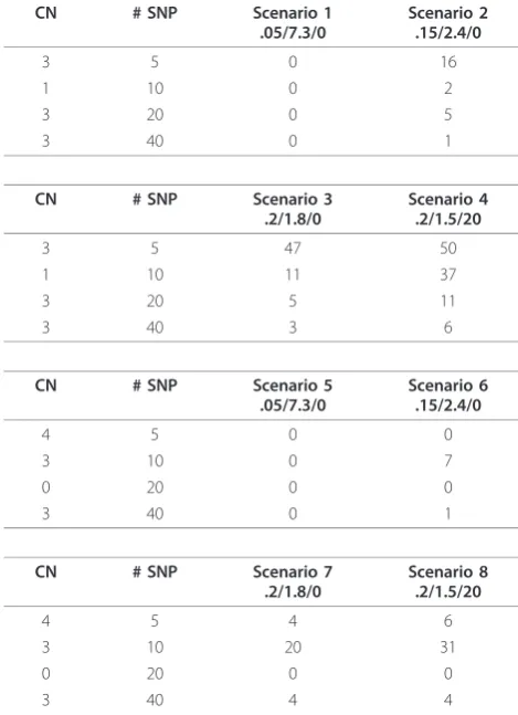
Table 1 shows misclassification rates (%) for eight dif-ferent scenarios. Tables 2 and 3 show false-negative and false-positive rates, respectively. We first discuss the misclassification (MC) rates in Table 1.

Scenarios 1-4:These scenarios assume the following

ordered copy number segments with number of SNPs given in parentheses: 2(10), 3(5), 2(50), 1(10), 2(50), 3 (20), 2(50), 3(40), 2(10). The widths of the copy number segments (5, 10, 20, 40, 50) correspond to those consid-ered by Rancoita et al. [20]. The SD and SNR are given on the log2 ratio scale under a true CN of 3. Since in this table we report misclassification rates, we do not

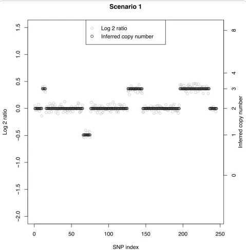
show the segments corresponding to a true copy num-ber of 2, which would be the false-positive rate (Table 3). The rows are ordered by segment as given above, excluding segments with a normal copy number. Figure 2 shows a typical data set under Scenario 1 in which the SNR of 7.3 leads to clearly non-overlapping log-ratios across the segments. In this case, the MC rate is 0% independent of CN aberration and number of SNPs

Table 1 Misclassification rates from simulation study.

CN # SNP Scenario 1

.05/7.3/0

Scenario 2 .15/2.4/0

3 5 0 16

1 10 0 2

3 20 0 5

3 40 0 1

CN # SNP Scenario 3

.2/1.8/0

Scenario 4 .2/1.5/20

3 5 51 50

1 10 11 37

3 20 9 11

3 40 6 6

CN # SNP Scenario 5

.05/7.3/0

Scenario 6 .15/2.4/0

4 5 6 87

3 10 0 14

0 20 0 0

3 40 0 9

CN # SNP Scenario 7

.2/1.8/0

Scenario 8 .2/1.5/20

4 5 77 98

3 10 31 31

0 20 0 0

3 40 17 4

The entry is the misclassification rate, expressed as a percentage, over 50 replicates of one chromosome. Eight scenarios were simulated and defined by the given combination of true CN, number SNPs within the region of aberration, and SD/SNR/percent contamination. The SD and SNR are given on the log2 ratio scale under a true CN of 3. The true CN profile for Scenarios 1-4 is CN(#SNPs): 2(10), 3(5), 2(50), 1(10), 2(50), 3(20), 2(50), 3(40), 2(10). The true CN profile for Scenarios 5-8 is CN(#SNPs):2(10), 4(5), 2(50), 3(10), 2(50), 0(20), 2 (50), 3(40), 2(10).

Table 2 False negative rates from simulation study.

CN # SNP Scenario 1

.05/7.3/0

Scenario 2 .15/2.4/0

3 5 0 16

1 10 0 2

3 20 0 5

3 40 0 1

CN # SNP Scenario 3

.2/1.8/0

Scenario 4 .2/1.5/20

3 5 47 50

1 10 11 37

3 20 5 11

3 40 3 6

CN # SNP Scenario 5

.05/7.3/0

Scenario 6 .15/2.4/0

4 5 0 0

3 10 0 7

0 20 0 0

3 40 0 1

CN # SNP Scenario 7

.2/1.8/0

Scenario 8 .2/1.5/20

4 5 4 6

3 10 20 31

0 20 0 0

3 40 4 4

The entry is the false-negative rate, expressed as a percentage, over 50 replicates of one chromosome.

See Table 1 for details.

Table 3 False positive rates from simulation study.

CN # SNP Scenario 1/5

.05/7.3/0

Scenario 2/6 .15/2.4/0

2 10 0 3

2 50 0 1

CN # SNP Scenario 3/7

.2/1.8/0

Scenario 4/8 .2/1.5/20

2 10 7 9

2 50 2 2

The entry is the false-positive rate, expressed as a percentage, over 50 replicates of one chromosome.

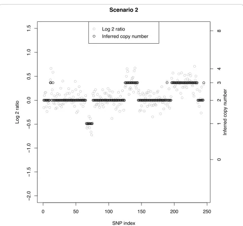
defining the respective segments. Scenarios 2, 3, and 4 have increasingly smaller SNRs and for a given true CN aberration the MC rate increases with decreasing SNR (left to right across columns). Figure 3 shows a data set under Scenario 2 with a SNR of 2.4. The overlap between CN classes is mild, but clear change points can still be observed when there are at least 10 SNPs. Here, a few of the CN = 3 cases between SNPs 11-15 are clas-sified as normals. Conversely, at about SNPs #190 and

250, normal CNs are classified as CN = 3. The largest MC rate (16%) under Scenario 2 is that corresponding to a segment with true CN = 3 and 5 SNPs. The other three cases under Scenario 2 with at least 10 SNPs have a MC rate of no more than 5%. Figures 4A and 4B show two data sets under Scenario 3 with a SNR under 2, namely SNR = 1.8. Figure 4A shows correct classification of 4 of 5 CN = 3 cases between SNPs 11-15, while Figure 4B shows all 5 of these CN = 3 cases misclassified as

Scenario 1

normals. However, Figure 4A shows more misclassifica-tions of the CN = 3 cases between SNPs 230 and 240 than that in Figure 4B. With at least 10 SNPs in a seg-ment, the MC rate is no more 11% under Scenario 3. Under Scenario 4 the SNR is 1.5 and as with Scenario 3 (SNR = 1.8) the MC rate is about 50% when only 5 SNPs define the segment. With a SNR as small as 1.5, a rela-tively large (> 10) number of SNPs are needed to accu-rately classify a copy number.

Scenarios 5-8:These represent the following ordered

copy number segments with number of SNPs in parenth-eses: 2(10), 4(5), 2(50), 3(10), 2(50), 0(20), 2(50), 3(40), 2 (10). As with Scenarios 1-4, for a given combination of

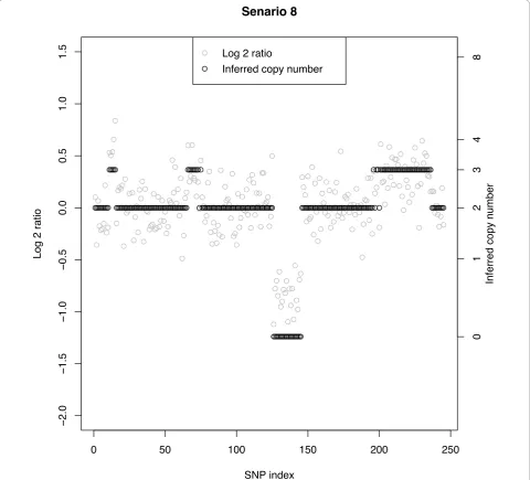
CN and number of SNPs in the segment, the MC rate increases with decreasing SNR. Segments with a larger number of SNPs also lead to smaller MC rates than those with fewer SNPs. One interesting comparison is that between row 1 of Scenarios 1-4 (CN = 3 with 5 SNPs) with row 1 of Scenarios 5-8 (CN = 4 with 5 SNPs). Figure 5 shows a sample data set from Scenario 8 and there we observe that all five SNPs with CN = 4 at positions 11-15 are classified as CN = 3. Examining the misclassifications across all 50 replicates for this configuration we found that the vast majority of SNPs with CN = 4 were labelled as a 3; hence, the misclassification rate of 98%. Note that the false-negative rate for this situation (Table 2 row 1,

Scenario 2

Scenario 8) was only 6%. On the other hand, the MC rate under Scenario 4 with CN = 3 with 5 SNPs was 50%, approximately half that for CN = 4 in Scenario 8. In gen-eral, larger copy number aberrations are more difficult to correctly identify than smaller ones. Indeed, the log scale shrinks the larger copy number ratios toward smaller ones, leading to misclassifications. Line 3 shows MC rates under a true copy number of 0. Figure 5 shows how distinct this aberration is from its neighbors regardless of the size of the SNR; the MC is constantly 0%.

Table 2 shows false-negative rates. Except for minor differences, the false-negative rates for Scenarios 1-4 are

the same as the broader misclassification rates (Table 1). This shows that most of the misclassifications in Scenar-ios 1-4 were losses and gains that were called normal. Where there are differences between Tables 1 and 2, we see that misclassification rates are at least as large as the false-negative rates as we would expect. It is worth not-ing that the aberrations studied in Scenarios 1-4 are neighbors of normal copy number, viz., CN = 3 is one additional copy and CN = 1 is one less copy. As such, it is not too surprising that the misclassification rates agreed with the false-negative rates. Especially in the presence of normal cell contamination we expect the

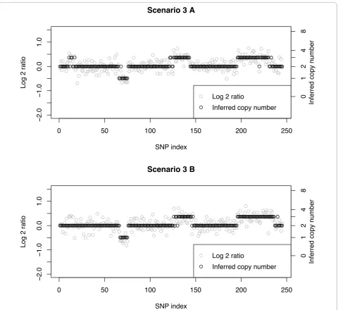
Scenario 3 A

Scenario 3 B

log-ratios to regress toward the mean value of 0. This is contrast to Scenarios 5-8, which include more extreme aberrations of CN = 0 and CN = 4. Comparing the mis-classification rates (Table 1) with the corresponding FN rates (Table 2), we see that the latter can be much smal-ler than the former. Large differences of MC vs FN rates are seen for CN = 4 in Scenarios 6 (87% vs 0%), 7 (77% vs 4%), and 8 (98% vs 6%). Taken together this implies that almost all of the misclassifications for CN = 4 were called as CN = 3 and very few as CN = 2. A manual cal-culation of the calls confirms this conclusion. Smaller differences between MC and FN rates occur in Scenario 6 with CN = 3 and 10 SNPs (line 2, Tables 1 and 2); the MC rate is 14% and the FN rate is 7%. Here, half of the

14% is due to normal calls and the other half to calls of CN = 4. In Scenario 7 with true CN = 3 and 10 SNPs the MC rate of 31% is 20% CN = 2 (false-negative) and 11% CN = 4. Similarly, the MC rates of 9% and 17% for Scenarios 6 and 7 with CN = 3 and 40 SNPs (line 4, Tables 1 and 2), respectively, are only due to false calls of CN = 2 and CN = 4. It is, therefore, seen that when a true copy number of 3 is misclassified, it tends to be called a CN = 4 with a smaller percentage of normal calls, CN = 2. And, as discussed above, a true CN = 4 tends to be called a 3 when misclassified. In this sense, if an investigator is only calling loss/normal/gain, even though misclassifications occur under true copy num-bers of 3 and 4, they would both be correctly called as

Senario 8

gains with a small percentage of CN = 2 (false-negative) calls. This is at least the behavior of the Bayes mixture model; other methods may apportion the misclassifica-tions differently. In all scenarios (1-8) we observe a mis-classification rate and a false-negative rate of 0% for CN = 0 and 20 SNPs. No matter the signal-to-noise ratio, the distribution of log-ratios for CN = 0 is well separated from the other copy number distributions and its call is constantly correct. For CN = 1, the misclassification rates and corresponding false-negative rates are equal, showing that when misclassified this copy number is called a nor-mal (false-negative). Table 3 shows false-positive (FP) rates defined as a true normal copy number being classi-fied as a gain or loss:P(CN≠2 |CN= 2). Since the two patterns of copy number structure differed only in their gain and loss patterns we combined the data for the nor-mal copy number segments. Thus the FP rates are based on 100 replicates instead of 50 as with the MC and FN rates in Table 1. As with the FN rate, for a fixed number of SNPs defining the normal segment, the FP positive rate increases with decreasing SNR. And, for a given combination of SNR and normal cell contamination, the FP rate decreases with an increasing number of SNPs in the segment. Under the most difficult configuration con-sidered, 10 SNPs with a SNR of 1.5 and 20% contamina-tion, the false-positive rate was only 9%.

Rancoita et al. [20] compared their mBPCR method with six other methods and found that in general no method, including their own, was able to detect aberra-tions of width 5-10 probes. Lai et al. [30] reached simi-lar conclusions. Use of alternative estimators for a certain covariance parameter led to the detection of these smaller segments, but this was accompanied by dividing larger segments into sub-segments. Our method, too, had trouble with regions defined by only 5 probes, although regions with 10 probes were fairly well identified unless the signal-to-noise ratio was on the order of 1.5.

Real Data Application

To further assess the Bayes mixture model, we analyzed Affymetrix 250Karray data from cancer patients who had either leukemia or ependymoma. Data were obtained from Texas Children’s Hospital, Houston, TX. In addition to comparing our results with the popular CNAG software, we also provide biological validation. Some of these cases, in fact, had karyotyping and FISH data for validation. Others were validated using quanti-tative PCR on selected regions and aCGH data. We also briefly comment on comparisons with some results from the PennCNV algorithm.

One important feature of the CNAG software used to estimate copy number is the fact that it adjusts the observed log-ratios for variation in GC content across the

probes. Integer copy numbers are subsequently inferred from the GC adjusted log-ratios using a hidden Markov model. To make comparable comparisons between the Bayes and the CNAG methods we applied the Bayes model to the GC adjusted log-ratios from CNAG. One relatively recent issue arising in the analysis copy number aberration detection is the so-called “genome wave” [11,12], a genome-wide spatial autocorrelation pattern in signal intensity data that may be confounded with the copy number profile across a chromosome. As a result the genome wave may lead to inflated false-positive rates in copy number calls. The genome wave has been consis-tently detected in both CGH and SNP based platforms. Diskin et al. [12] and the references therein describe possi-ble genomic features underlying the wave effect and pre-processing methods to remove the wave effect prior to the analysis of copy number. It has been fairly well established that an adjustment for GC content largely removes the wave effect from the signal intensities [12]. Since we are using GC adjusted log-ratios from CNAG for the real data application we did not expect to observe a wave effect in our data and indeed none was present as shown in [Addi-tional file 1].

validation would be needed to discriminate this apparent difference.

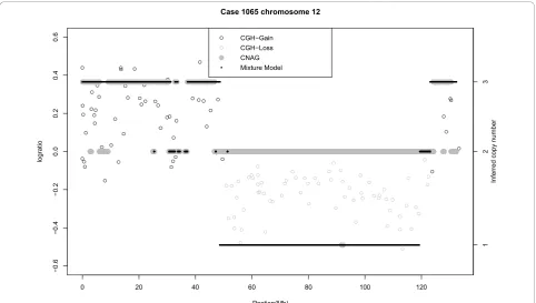
In the next example we consider an ependymoma case (#1065). Figure 7 shows chromosome 12 for this case. Both methods infer CN = 3 for much of the region from 0 to 30 Mb, although prior to the centromere located at 35 Mb there is a signal for CN = 2. The main difference between the two algorithms centers on the segment from approximately 45 to 120 Mb. This seg-ment is identified as CN = 2 by CNAG and CN = 1 by the Bayes algorithm. In order to validate this result we performed qPCR on two regions in this stretch: at approximately 55 Mb, and 110 Mb. The qPCR average (95% confidence interval) copy numbers for these two

regions were 1.43 (1.2, 1.71) and 1.55 (1.33, 1.81), respectively. These validation results support the loss identified by the Bayes method. Given that the distribu-tion of the log-ratios from 45-120 Mb agrees with those at 55 Mb and 110 Mb we conclude that the Bayes method has correctly identified a loss from 45-120 Mb. There is also a discrepancy at the end of the chromo-some. The Bayes method infers a contiguous gain of CN = 3 (125-134 Mb), whereas CNAG has a gain (123-130 Mb) followed by a normal region (130-134 Mb). qPCR validation was performed at locations 127 Mb and 132 Mb and we found means of (95% confidence interval) of 2.81 (2.48, 3.18) and 2.36 (1.96, 2.85), respectively. The first qPCR result suggests a CN of 3. The second result

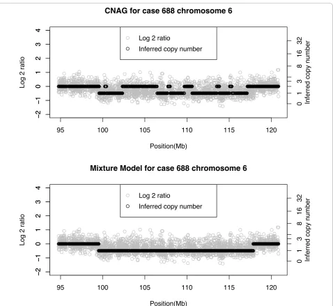
CNAG for case 688 chromosome 6

!

!

Mixture Model for case 688 chromosome 6

!

!

is somewhat less conclusive as CN = 2 is just inside the confidence interval, which is approximate. To further validate this case, we therefore generated aGCH data via an aCGH platform with 2,621 BACs and a resolution of 3 Mb. Having analyzed the aCGH data with the GLAD software from Bioconductorhttp://www.bioconductor. org/, Figure 8 shows the aCGH results overlayed by the Bayes and CNAG results. The aCGH data show a gain of CN = 3 from the beginning of the chromosome to the centromere at 35 Mb. With the exception of a few

small regions both the Bayes and CNAG methods agree with GLAD in this region. From the beginning of the q

arm to 45 Mb all three methods show CN = 3. From 45 Mb to 120 Mb, GLAD clearly indicates a loss, and from 120 Mb to the end at 134 Mb a gain. It thus appears that the Bayes method correctly identified a gain at the end of the chromosome, whereas CNAG inferred a nor-mal copy number.

In the two real cases (688 and 1065) discussed thus far, the Bayesian method showed regions of loss, a 19

CNAG for case 1065 chromosome 12

Mixture Model for case 1065 chromosome 12