Conductance from Non-perturbative Methods I

City, University of London Institutional Repository

Citation

:

This is the published version of the paper.

This version of the publication may differ from the final published

version.

Permanent repository link: http://openaccess.city.ac.uk/13901/

Link to published version

:

Copyright and reuse:

City Research Online aims to make research

outputs of City, University of London available to a wider audience.

Copyright and Moral Rights remain with the author(s) and/or copyright

holders. URLs from City Research Online may be freely distributed and

linked to.

City Research Online: http://openaccess.city.ac.uk/ [email protected]

arXiv:cond-mat/0210599v1 28 Oct 2002

PrHEP unesp2002

Conductance from Non-perturbative Methods I

Olalla A. Castro-Alvaredo and Andreas Fring∗

Institut f¨ur Theoretische Physik, Freie Universit¨at Berlin, Arnimallee 14, D-14195 Berlin, Germany

E-mail: [email protected],[email protected]

Abstract:_{We investigate different methods to compute the DC conductance in a}

quan-tum wire doped with some impuritied by exploiting the integrability of the theories under consideration. As an essential ingredient in all methods we evaluate the reflection and transmission amplitudes of the impurities for a variety of defects. When the impurities in the wire are coupled to an external three dimensional laser field, we predict the generation of harmonic emission spectra. We propose a modified version of the well-known Kubo for-mula, which incorporates the impurities of the system and evaluate the current-current two-point correlation function it involves with the help of a form factor expansion. A comparison with the corresponding quantities computed in a Landauer transport theory picture is carried out in part II.

The work I want to report about is based on a series of papers [1, 2, 3, 4, 5, 6] with an emphasis on the first two. Olalla Castro-Alvaredo will present the second part of this talk.

1. Generalities on conductance

In the context of 1+1 dimensional quantum field theories an impressive arsenal of non-perturbative techniques has been developed over the last 25 years. The original motivation was to use the lower dimensional set up as a testing ground for general conceptual ideas and possibly to apply them in the context of string theory, such that most of the work in this area can be characterized very often as rather formal. However, lately the experimental techniques have advance to such an extent that one might realistically hope to measure various quantities which can be predicted based on these approaches.

One of those quantities, which is particularly easy to access, is the conductance (con-ductivity). It can be measured in general directly without perturbing very much the behaviour of the system, e.g. a rigid-lattice bulk metal, such that the uncertainty of ex-perimental artefacts is reduced to a minimum. Indeed, there have been some fairly recent

PrHEP unesp2002

explain these data theoretically and possibly inspire more experiments of a similar type. There exist two main theoretical descriptions to compute the conductance, the Kubo formula [8, 9], which is the outcome of a dynamical linear-response theory and the Landauer-B¨uttinger theory [10], which is a semi-classical transport theory. The main purpose of the work I want to present is a comparison between these two descriptions by employing non-perturbative methods of 1+1 dimensional integrable models. It is in this sense the wording non-perturbative is to be understood, that is despite the fact that the overall theoretical description is of a perturbative nature, within these frameworks we use non-perturbative methods. I will concentrate on our proposal of a generalized Kubo formula and in the second part, presented by Olalla Castro-Alvaredo, the computations within the Landauer-B¨uttinger transport theory framework will be presented.

I will start by anticipating the quantities we have to compute. The system we consider is a one dimensional quantum wire doped with some impurities (defects). For the time being we leave the theory describing the wire and also the nature of the impurities unspecified. In linear response theory one essentially needs the Fourier transform of the current-current two-point correlation function. This so-called Kubo formula has been adopted to a situation with a boundary [11]. Since this only captures effects coming from the constriction of the wire a generalization to a set up with defects was needed, which we proposed in [1] as

Gα(T) =₋lim

ω→0

1 2ωπ2

Z ∞

−∞

dt eiωt _hJ(t)ZαJ(0)i_T,m. (1.1)

Here the defect operatorZα enters in-between the two local currentsJ within the

temper-atureT and mass mdependent correlation function. The Matsubara frequency is denoted by ω.

The other possibility of determining the conductance which we want to study, is a generalization of the Landauer-B¨uttinger transport theory picture. Within this framework a proposal for the conductance through a quantum wire with a defect (impurity) has been made in [12, 13]

Gα(T) =X

i

lim

(µl i−µri)→0

qi

2

Z ∞

−∞

dθhρr_i(θ, T, µl_i)_|T_iα(θ)_|2₋ρ_ir(θ, T, µr_i)_|T˜_iα(θ)_|2i, (1.2)

which we only modify to accommodate parity breaking. This means we allow the trans-mission amplitudes for a particle of type iwith charge qi passing with rapidity θ through

a defect of typeα from the leftT_iα(θ) and right ˜T_iα(θ) to be different. The density distri-bution functionρr

i(θ, T, µi) depends on the temperature T, and the potential at the leftµli

and rightµr

i constriction of the wire.

The main quantities we have to compute before we can evaluate (1.1) and (1.2) are the transmission amplitudesTi, the current-current correlation functionsh. . .iT,m and the

density distributions ρi. We obtain all of them non-perturbatively, the T’s by means of

PrHEP unesp2002

2. Impurity systems

2.1 Constraints from the generalized Yang-Baxter equations

Let me start with the evaluation of the transmission amplitudes, since they will be required in (1.1) as well as in (1.2). One of the great advantages of integrability in 1+1 dimensional models is that the n-particle scattering matrix factorises into two-particle S-matrices, which can be determined by some constraining equations such as the Yang-Baxter [19] and boot-strap equations [20]. Similar equations hold in the presence of a boundary [21, 22, 23] or a defect [24, 4]. It is clear that with regard to the conductance a situation with a pure boundary, i.e. non-trivial effects on the constrictions, or purely transmitting defects will be rather uninteresting and we would like to consider the case when R and T are simultaneously non-vanishing. Unfortunately, it will turn out that for that situation the Yang-Baxter equations are so constraining that not many integrable theories will be left to consider. Thus this section serves essentially to motivate the study of the free Fermion, which after all is very close to a realistic system of electrons propagating in quantum wires. We label now particle types by Latin and degrees of freedom of the impurity by Greek letters, the bulk scattering matrix byS, and the left/right reflection and transmission am-plitudes of the defect byR/R˜ and T /T˜, respectively. Then the transmission and reflection amplitudes are constrained by the “unitarity” relations

Rjβ_iα(θ)R_jβkγ(₋θ) +T_iαjβ(θ) ˜T_jβkγ(₋θ) = δk_iδ_αγ, (2.1)

R_iαjβ(θ)T_jβkγ(₋θ) +T_iαjβ(θ) ˜Rkγ_jβ(₋θ) = 0, (2.2) and the crossing-hermiticity relations

R_α_¯(θ) = ˜R_α_¯(₋θ)∗ =Sj¯(2θ) ˜Rαj(iπ−θ), (2.3)

T_¯α(θ) = ˜T_¯α(₋θ)∗ = ˜T_jα(iπ₋θ). (2.4) The equations (2.1) and (2.2) also hold after performing a parity transformation, that is forR_↔R˜ and T _↔T˜.

Depending now on the choice of the initial asymptotic condition one can derive the following two non-equivalent sets of generalized Yang-Baxter equations by exploiting the associativity of the extended Zamolodchikov-Faddeev algebra [21, 22, 23, 24, 4]

S(θ12)[I⊗Rβα(θ1)]S(ˆθ12)[I⊗Rγβ(θ2)] = [I⊗Rαβ(θ2)]S(ˆθ12)[I⊗Rγβ(θ1)]S(θ12), (2.5)

S(θ12)[I⊗Rβα(θ1)]S(ˆθ12)[I⊗T_βγ(θ2)] =Rγ_β(θ1)⊗Tαβ(θ2), (2.6)

S(θ12)[Tαβ(θ2)⊗T_βγ(θ1)] = [Tαβ(θ1)⊗T_βγ(θ2)]S(θ12), (2.7)

and

R_αβ(θ1)⊗R˜γβ(θ2) = Rγβ(θ1)⊗R˜αβ(θ2), (2.8)

[T_αβ(θ2)⊗I]S(ˆθ12)[ ˜Rγ_β(θ1)⊗I]S(θ12) = T_βγ(θ2)⊗R˜βα(θ1), (2.9)

[I_⊗T˜_αβ_{(θ2)]S(ˆθ12)[}I_⊗Rγ

β(θ1)]S(θ12) = Rβα(θ1)⊗T˜_βγ(θ2), (2.10)

PrHEP unesp2002

ij = AkiBjl for the tensor product and abbreviated

the rapidity sum ˆθ12=θ1+θ2 and differenceθ12=θ1−θ2. Once again the same equations

also hold forR_↔R˜ and T _↔T˜.

Apart from some discrepancies in the indices the equations (2.5)-(2.7) correspond to a more simplified, in the sense that there were no degrees of freedom in the defect and parity invariance is assumed, set of equations considered previously in [24]. For diagonal scattering it was argued in [24] that one can only have reflection and transmission simultaneously when

S =_±1. In [4] a more general set up which includes all degrees of freedom was studied. A second set of equations (2.8)-(2.11), which is not equivalent to (2.5)-(2.7) was found. It was shown that in the absence of degrees of freedom in the defect no theory which has a non-diagonal bulk scattering matrix admits simultaneous reflection and transmission. This result even holds for the completely general case including degrees of freedom in the defect upon a mild assumption on the commutativity of R and T in these variables. It was further shown that besidesS=_±1 also the Federbush model [25] and the generalized coupled Federbush models [6] allow for R₆= 0 and T ₆= 0.

2.2 Multiple impurity systems

The most interest situation in impurity systems arises when instead of a single one considers multiple defects, since that leads to the occurrence of resonance phenomena and when the number of defects tends to infinity even to band structures. Assuming that the distance between the defects is small in comparison to the length of the wire one can easily construct the transmission and reflection amplitudes of the multiple defect system from the knowledge of the corresponding quantities in the single defect system. For instance for two defects one obtains

T_iαβ(θ) = T

α i (θ)T

β i (θ)

1₋Rβ_i(θ) ˜Rα_i(θ), R

αβ

i (θ) =Rαi(θ) +

Rβ_i(θ)T_iα(θ) ˜T_iα(θ)

1₋Rβ_i(θ) ˜Rα_i(θ) , (2.12) ˜

T_iαβ(θ) = T˜

α i (θ) ˜T

β i (θ)

1₋Rβ_i(θ) ˜Rα_i(θ), ˜

Rαβ_i (θ) = ˜Rβ_i(θ) +R

α i(θ)T

β i (θ) ˜T

β i (θ)

1₋Rβ_i(θ) ˜Rα_i(θ) . (2.13) These expressions allow for a direct intuitive understanding, for instance we note that the term [1₋R_iβ(θ) ˜Rα_i(θ)]−1 =P∞

n=1(R

β

i(θ) ˜Rαi(θ))n simply results from the infinite number

of reflections which we have in-between the two defects. This is of course well known from Fabry-Perot type devices of classical and quantum optics. For the caseT = ˜T , R = ˜R the expressions (2.12) and (2.13) coincide with the formulae proposed in [26]. When absorbing the space dependent phase factor into the defect matrices, the explicit example presented in [24] for the free Fermion perturbed with the energy operator agree almost forT = ˜T , R= ˜R

with the general formulae (2.12). They disagree in the sense that the equality of Rαβ_i (θ) and ˜Rαβ_i (θ) does not hold for genericα, β as stated in [24].

It is now straightforward to generalize the expressions for an arbitrary number of defects, sayn, in a recursive manner

T_i~α(θ) = T

α1...αk

i (θ)T

αk+1...αn

i (θ)

1₋R˜α1...αk

i (θ)R

αk+1...αn

i (θ)

PrHEP unesp2002

i (θ) +

Rαk+1...αn

i (θ)Tiα1...αk(θ) ˜Tiα1...αk(θ)

1₋R˜α1...αk

i (θ)R

αk+1...αn

i (θ)

, 1< k < n . (2.15)

We encoded here the defect degrees of freedom into the vector α~=_{α1,· · ·, αn}. Similar

expressions also hold for ˜Tα~

i (θ) = ˜Tiα1...αn(θ) and ˜Ri~α(θ) = ˜Rαi1...αn(θ).

Alternatively, we can define, in analogy to standard quantum mechanical methods (see e.g. [14]), a transmission matrix which takes the particle i from one side of the defect of type α to the other

Miα(θ) =

Tα

i (θ)−1 −Rαi(θ)Tiα(θ)−1

−Rα_i(₋θ)T_iα(₋θ)−1 T_iα(₋θ)−1

!

. (2.16)

Then alternatively to the recursive way (2.14) and (2.15), we can also compute the multi-defect transmission and reflection amplitudes as

T_i~α(θ) =

n Y k=1

Miαk(θ)

!−1

11

, R_i~α(θ) =₋

n Y k=1

Miαk(θ)

!

12

n Y k=1

Miαk(θ)

!−1

11

. (2.17)

This formulation has the virtue that it is more suitable for numerical computations, since it just involves matrix multiplications rather than recurrence operations. In addition it allows for an elegant analytical computation of the band structures for n _{→ ∞}, which I will however not comment upon further in this talk.

2.3 Constraints from potential scattering theory

As we argued in section 2.1., in order to obtain a non-trivial conductance we are lead to consider free theories, possibly with some exotic statistics. Trying to be as close as possible to some realistic situation, i.e. electrons, we consider first the free Fermion, which with a line of defect was first treated in [27]. Thereafter it has also been considered in [28, 24] and [29] from different points of view. In [27, 28, 24] the defect line was taken to be of the form of the energy operator and in [29] also a perturbation in form of a single Fermion has been considered. In [1] we treated a much wider class of possible defects.

Let us consider the Lagrangian density for a complex free Fermionψ withℓdefects1

L= ¯ψ(iγµ∂µ−m)ψ + ℓ X n=1

Dαn_{( ¯ψ, ψ, ∂}

tψ, ∂¯ tψ)δ(x−xn). (2.18)

The defect is described here by the functions _Dαn_{( ¯ψ, ψ, ∂}

tψ, ∂¯ tψ), which we assume to

be linear in the Fermi fields ¯ψ,ψ and their time derivatives. We can now proceed in

1_{We use the conventions:}

xµ = (x0, x1), pµ= (mcoshθ, msinhθ), g00=−_g11_=ε01₌−_ε10_{= 1,}

γ0 = 0 1

1 0 !

, γ1= 0 1

−_{1 0}

!

, γ5=γ0γ1, ψα=

ψα(1)

ψα(2) !

, ψ¯α=ψα†γ0.

We adopt relativistic units 1 =c=~_=m≈_e2_{137 as mostly used in the particle physics context rather}

PrHEP unesp2002

and construct the amplitudes by adequate matching conditions on the field. We consider first a single defect at the origin which suffices, since multiple defect amplitudes can be constructed from the single defect ones, according to the arguments of the previous section. We decompose the fields of the bulk theory as ψ(x) = Θ(x) ψ+(x) + Θ(−x) ψ−(x), with Θ(x) being the Heavyside unit step function, and substitute this ansatz into the equations of motion. As a matching condition we read off the factors of the delta function and hence obtain the constraints

iγ1(ψ+(x)−ψ−(x))|x=0 =

∂_D ∂ψ¯(x)

x=0

− _∂t∂

∂_D ∂(∂tψ¯(x))

x=0

. (2.19)

We then use for the left (₋) and right (+) parts ofψthe well-known Fourier decomposition of the free field

ψf_j(x) =

Z

dθ √

4π

aj(θ)uj(θ)e−ipj·x+a†¯(θ)vj(θ)e

ipj·x

, (2.20)

with the Weyl spinors

uj(θ) =−iγ5vj(θ) = r

mj

2

e−θ/2

eθ/2

!

(2.21)

and substitute them into the constraint (2.19). Treating the equations obtained in this manner componentwise, stripping off the integrals, one can bring them thereafter into the form

aj,−(θ) =Rj(θ)aj,−(−θ) +Tj(θ)aj,+(θ) , (2.22)

which defines the reflection and transmission amplitudes in an obvious manner. When parity invariance is broken, the corresponding amplitudes from the right to the left do not have to be identical and we also have

aj,+(−θ) = ˜Tj(θ)aj,−(−θ) + ˜Rj(θ)aj,+(θ). (2.23)

The creation and annihilation operators a†_i(θ) and ai(θ) satisfy the usual fermionic

anti-commutation relations _{ai(θ1), aj(θ2)} = 0, {ai(θ1), a†j(θ2)} = 2πδijδ(θ12). In this way

one may construct the R’s and T’s for any concrete defect which is of the generic form as described in (2.18). After the construction one may convince oneself that the expres-sions found this way indeed satisfy the consistency equations like unitarity (2.1), (2.2) and crossing (2.3), (2.4). Unfortunately the equations (2.1)-(2.4) can not be employed for the construction, since they are not restrictive enough by themselves to determine theR’s and

T’s. We consider now some concrete examples:

2.3.1 Impurities of Luttinger liquid type _D( ¯ψ, ψ) = ¯ψ(g1+g2γ0)ψ

Luttinger liquids [30] are of great interest in condensed matter physics, which is one of the motivations for our concrete choice of the defect _D( ¯ψ, ψ) = ¯ψ(g1 +g2γ0)ψ. When

PrHEP unesp2002

outlined above, we compute the related transmission and reflection amplitudes

Rj(θ, g1, g2,−y) = ˜Rj(θ, g1, g2, y) =

4i(g2+g1coshθ)e2iymsinhθ

(4 +g2₁₋g₂2) sinhθ₋4i(g1+g2coshθ)

, (2.24)

R¯(θ, g1, g2,−y) = ˜R¯(θ, g1, g2, y) = 4i(g1−g2coshθ)e

−2iymsinhθ

(4 +g2

1−g22) sinhθ−4i(g1−g2coshθ)

, (2.25)

Tj(θ, g1, g2) = ˜Tj(θ, g1, g2) =

(4 +g2

2 −g21) sinhθ

(4 +g2

1−g22) sinhθ−4i(g1+g2coshθ)

, (2.26)

T¯(θ, g1, g2) = ˜T¯(θ, g1, g2) =

(4 +g2

2 −g21) sinhθ

(4 +g2

1−g22) sinhθ−4i(g1−g2coshθ)

. (2.27)

In the limit limg2→0D( ¯ψ, ψ) = g1ψψ¯ , we recover the related results for the T /T˜’s and

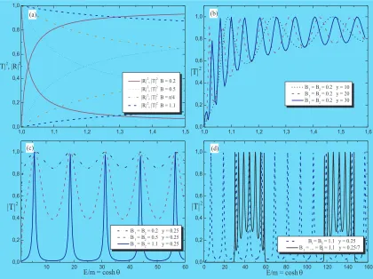
R/R˜’s for the energy defect operator. For this type of defect we present _|T_|2 and _|R_|2 in figure 1 with varying parameters in order to illustrate some of the characteristics of these functions.

Figure 1: (a) Single defect with varying coupling constant. |T|2

and |R|2

correspond to curves starting at 0 and 1 of the same line type, respectively. (b) Double defect with varying distancey . (c) Double defect with varying effective coupling constantB= arcsin(−4g1/(4 +g12)). (d) Double

PrHEP unesp2002

typical resonances of a double defect, which become stretched out and pronounced with re-spect to the energy when the distance becomes smaller and the coupling constant increases, respectively. Part (d) exhibits a general feature, that is when the number of defects is in-creased, for fixed distance between the outermost defects, the resonances become more and more dense in that region such that one may speak of energy bands.

2.3.2 The defect _D( ¯ψ, ψ, ∂tψ, ∂¯ tψ) =ig/2( ¯ψ∂tψ−∂tψψ¯ )

This type of defect reminds on the first non-trivial charge occurring in the free Fermion model. In this case we compute by the same means the related transmission and reflection amplitudes to

˜

Rα_j(θ, y) = R_¯α(θ, y) =Rα_j(θ,₋y) = ˜Rα_¯(θ,₋y) = −4igcoshθe

2iymsinhθ

4ig+ tanhθ(4 +g2_cosh2_θ),(2.28)

T_jα(θ) = ˜T_jα(θ) =T_¯α(θ) = ˜T_¯α(θ) = (4−g

2_cosh2_{θ) tanhθ}

4ig+ tanhθ(4 +g2_cosh2_θ). (2.29)

In [1] we also computed the T /T˜’s and R/R˜’s for other types of defects, such as D = gψγ¯ 1_{ψ, D = gψγ}¯ 5_{ψ, D = gψ}¯_(γ1 _±γ5_{)ψ . . . As an overall conclusion we observed}

that all possible types of parity breaking, that is T ₆= ˜T; R ₆= ˜R or T ₆= ˜T; R = ˜R, etc., do occur. We also confirm a general principle one knows well from quantum mechanics, namely that parity is preserved when the potential is real, that is in this case the defect satisfies_D∗ =_D.

2.4 Impurities coupled to laser fields

Let us now consider a more complex situation in which a three dimensional laser field hits the quantum wire polarized in such a way that it has a vector field component along the wire. Since the work of Weyl [32], one knows that matter may be coupled to light by means of a local gauge transformation, which reflects itself in the usual minimal coupling prescription, i.e. ∂µ → ∂µ−ieAµ, with Aµ being the vector gauge potential. The free

Fermions in the wire are then described by the Lagrangian density

LA= ¯ψ(iγµ∂µ−m+eγµAµ)ψ . (2.30)

When the laser field is switched on, we can solve the equation of motion associated to (2.30)

(iγµ∂µ−m+eγµAµ)ψ= 0 (2.31)

by a Gordon-Volkov type solution [33]

ψ_jA(x, t) = exp

ie

Z x

dsA1(s, t)

ψf_j(x, t) = exp

ie

Z t

dsA0(x, s)

ψf_j(x, t). (2.32)

PrHEP unesp2002

A(t) :=A1(t) =

1

x

Z t

0

dsA0(s) =−

1 2

Z t

0

dsE(s) =₋E0 2

Z t

0

dsf(s) cos(ωs) (2.33)

withf(t) being an arbitrary enveloping function equal to zero fort <0 andt > τ, such that

τ denotes the pulse length. In the following we will always take f(t) = Θ(t)Θ(τ ₋t) , with Θ(x) being again the Heavyside unit step function. The second equality in (2.33),A0(x, t) =

xA˙(t), follows from the fact that we have to solve (2.32).

I want to comment on the validity of the dipole approximation in this context. It consists usually in neglecting the spatial dependence of the laser field, which is justified when xω < c = 1, where x is a representative scale of the problem considered. In the context of atomic physics this is typically the Bohr radius. In the problem investigated here, this approximation has to hold over the full spatial range in which the Fermion follows the electric field. We can estimate this classically, in which case the maximal amplitude is

eE0/ω2 and therefore the following constraint has to hold

eE0

ω

2

= 4Up <1, (2.34)

for the dipole approximation to be valid. Due to the fact thatx is a function ofω, we have now a lower bound on the frequency rather than an upper one as is more common in the context of atomic physics. We have also introduced here the ponderomotive energy Up for

monochromatic light, that is the average kinetic energy transferred from the laser field to the electron in the wire.

The solutions to the equations of motion of the free system and the one which includes the laser field are then related by a factor similar to the gauge transformation from the length to the velocity gauge

ψA_j (x, t) = exp [ixeA(t)]ψf_j(x). (2.35) In an analogous fashion one may use the same minimal coupling procedure also to couple in addition the laser field to the defect. One has to invoke the equation of motion in order to carry this out. For convenience we assume now that the defect is linear in the fields ¯ψ

and ψ. The Lagrangian density for a complex free Fermion ψwith ℓdefects _Dα( ¯ψ, ψ, Aµ)

of type αat the position xn subjected to a laser field then reads

LAD=LA+ ℓ X n=1

Dαn_{( ¯ψ, ψ, A}

µ)δ(x−xn). (2.36)

Considering for simplicity first the case of a single defect situated at x = 0, the solution to the equation of motion resulting from (2.36) is taken to be of the form ψA_j (x, t) = Θ(x)ψ_j,A₊(x, t) + Θ(₋x)ψA_j,−(x, t) , which means as before we distinguish here by notation the solutions (2.35) on the left and right of the defect,ψ_j,A₋(x, t) andψ_j,A₊(x, t), respectively. Proceeding as before, the matching condition reads now

iγ1(ψA_j,+(x, t)₋ψA_j,−(x, t))_|x=0 =

∂_DAD( ¯ψ, ψ, Aµ)

∂ψ¯A j (x, t)

x=0

PrHEP unesp2002

θ andg also depend on the characteristic parameters of the laser field

T(θ, g, E0, ω, t) and R(θ, g, E0, ω, t). (2.38)

With regard to the main theme of this talk, it is clear that the laser field can be used to control the conductance. For instance defects which have transmission amplitudes of the form as the solid line in figure 1 (c), can be used as optically controllable switching devices. I want to deviate now slightly from the main line of argument and report briefly on an interesting phenomenon one can predict with solutions of the type (2.38).

2.5 Harmonic generation

Let me first briefly explain what harmonics are. The first experimental evidence can be traced back to the early sixties [34]. Franken et al found that when hitting a crystalline quartz with a weak ultraviolet laser beam of frequencyω, it emits a frequency which is 2ω. Generalizing this phenomenon to higher multiples, one says nowadays that high harmonics generation is the non-linear response of a medium (a crystal, an atom, a gas, ...) to a laser field. Harmonic generation is important, since it allows to convert infrared input radiation of frequencyω into light in the extreme ultraviolet regime whose frequencies are multiples of ω (even up to order _∼1000, see e.g. [35] for a recent review). A typical experimental spectrum is presented in figure 2.

In gases, composed of atoms or

Figure 2:Harmonic spectrum for Neon for a Ti:Sa laser with λ = 795nm. Measured at the Max Born Institut Berlin [36]

small molecules, this phenomenon is well-understood and, to some extent, even controllable in the sense that the frequency of the highest harmonic, the so-called “cut-off”, visible in fig-ure 2, can be tuned as well as the in-tensities of particular groups of har-monics. In more complex systems, however, for instance solids, or larger molecules, high-harmonic generation is still an open problem. This is due to the fact that, until a few years ago, such systems were expected not to survive the strong laser fields one needs to produce such effects.

PrHEP unesp2002

harmonics from solid state devices and as a prototype of such a system we study a quantum wire coupled to the laser field in the way described in section 2.4.

In order to answer that question, we first have to study the spectrum of frequencies which is filtered out by the defect while the laser pulse is non-zero. The Fourier transforms of the reflection and transmission probabilities provide exactly this information

T(Ω, θ, E0, ω, τ) =

1

τ

Z τ

0

dt_|T(θ, E0, ω, t)|2cos(Ωt), (2.39)

R(Ω, θ, E0, ω, τ) =

1

τ

Z τ

0

dt_|R(θ, E0, ω, t)|2cos(Ωt). (2.40)

When parity is preserved for the reflection and transmission amplitudes, that is for real defects with_D∗_{=D, we have|T|}2_+|R|2 _{= 1, and it suffices to considerT in the following.}

2.5.1 Type I defects

Many features can be understood analytically. Taking the laser field in form of monochro-matic light in the dipole approximation (2.33), we may naturally assume that the trans-mission probability for some particular defects can be expanded as

|TI(θ, Up, ω, t)|2 =

∞

X k=0

t2k(θ)(4Up)ksin2k(ωt). (2.41)

We shall refer to defects which admit such an expansion as “type I defects”. Assuming that the coefficients t2k(θ) become at most 1, we have to restrict our attention to the regime

4Up <1 in order for this expansion to be meaningful for all t. Note that this is no further

limitation, since it is precisely the same constraint as already encountered for the validity of the dipole approximation (2.34). The functional dependence of (2.41) will turn out to hold for various explicit defects considered below. Based on this equation, we compute for such type of defect

TI(Ω, θ, Up, ω, τ) =

∞

X k=0

(2k)!(Up)ksin(τΩ)t2k(θ)

τΩQk_l=1[l2_−(Ω/2ω)2_] . (2.42)

It is clear from this expression that type I defects will preferably let even multiples of the basic frequencyω pass, whose amplitudes will depend on the coefficients t2k(θ). When we

choose the pulse length to be integer cycles, i.e. τ = 2πn/ω for n _∈Z_{, the expression in} (2.42) reduces even further. The values at even multiples of the basic frequency are simply

TI(2nω, θ, Up) = (−1)n

∞

X k=0

t2k(θ) (Up)k 2k

k₋n

!

, (2.43)

which becomes independent of the pulse length τ. Notice also that the dependence on

E0 and ω occurs in the combination of the ponderomotive energy Up. Further statements

require the precise form of the coefficients t2k(θ) and can only be made with regard to a

PrHEP unesp2002

2.5.2 Type II defects

Clearly, not all defects are of the form (2.41) and we have to consider also expansions of the type

|TII(θ, E0/e, ω, t)|2 =

∞

X k,p=0

tp_2k(θ)E

2k+p

0

ω2k cos

p_{(ωt) sin}2k_{(ωt). (2.44)}

We shall refer to defects which admit such an expansion as “type II defects”. In this case we obtain

TII(Ω, θ, E0/e, ω, τ) =

∞ X k,p=0 p X l=0 p l !

Ω sin(τΩ) (₋1)l+1_{τ ω}2+2kE

2k+2p

0 ×     

(2k+ 2l)!t2₂p_k(θ)

k+l Q q=0

[(2q)2₋₍Ω

ω)2]

+ (2k+ 2l)!t

2p+1 2k (θ)E0 k+l+1

Q q=1

[(2q₋1)2₋₍Ω

ω)2]      . (2.45)

We observe from this expression that type II defects will filter out all multiples of ω. For the pulse being once again of integer cycle length, this reduces to

TII(2nω, θ, Up, E0) =

∞ X k,p=0 p X l=0

(₋1)l+nt

2p

2k(θ)

22l−2p (Up)

k+p_E2p

0

p l

!

2k+ 2l k+l₋n

!

(2.46)

and

TII((2n−1)ω, θ, E0/e) =

∞ X k,p=0 p X l=0

(₋1)l+n+1t

2p+1 2k (θ)

22l−2p+1 (Up)

k+p

× p

l

!

(2k+ 2l)!(2n₋1)E2₀p+1

(l+k₋n+ 1)!(l+n+k)!, (2.47)

which are again independent ofτ. We observe that in this case we can not combine the E0

and ω into a Up.

2.5.3 One particle approximation

In spite of the fact that we are dealing with a quantum field theory, it is known that a one particle approximation to the Dirac equation is very useful and physically sensible when the external forces vary only slowly on a scale of a few Compton wavelengths, see e.g. [43]. We may therefore define the spinor wavefunctions

Ψj,u,θ(x, t) : =ψjA(x, t)

a

†

j(θ) E q

2π2_p0

j

= e −i~pj·~x

q

2πp0_j

uj(θ) (2.48)

Ψj,v,θ(x, t)† : =ψjA(x, t)†

a

†

j(θ) E q

2π2_p0

j

= e −i~pj·~x

q

2πp0_j

PrHEP unesp2002

ΨA_i,u,θ(x, t) : =ψ_iA(x, t)

a

†

i,−(θ)

E q

2π2_p0

i

= Θ(₋x) [Ψi,u,θ(x, t) + Ψi,u,−θ(x, t)Ri∗(θ)]

+Θ(x)T_i∗(θ)hΨi,u,θ(x, t) + Ψi,u,−θ(x, t) ˜R∗i(−θ)

i

(2.50)

and the same function with u _→ v. Since this expression resembles a free wave, it can not be normalized properly and we have to localize the wave in form of a wave packet by multiplying with an additional function, ˜g(p, t) in (2.20) and its counterpart g(x, t) in (2.50), typically a Gaußian. Then for the function ΦA_i,u,θ(x, t) =g(x, t)ΨA_i,u,θ(x, t), we can achieve that_kΦ_k= 1.

2.5.4 Harmonic spectra

We are now in the position to determine the emission spectrum for which we need to compute the absolute value of the Fourier transform of the dipole moment

Xj,u,θ(Ω) =

Z τ

0

dt DΦA_j,u,θ(x, t)†xΦA_j,u,θ(x, t)EexpiΩt

. (2.51)

We localize now the wave packet in a region much smaller than the classical estimate for the maximal amplitude the electron will acquire when following the laser field. We achieve this with a Gaußiang(x, t) = exp(₋x2/∆), where ∆_≪eE0/ω2.

2.5.5 An example: Impurity of energy operator type

As mentioned this type of defect, i.e. _D( ¯ψ, ψ) =gψψ¯ (x) can be obtained in a limit from the defect discussed in section 2.3.1. Coupling the vector potential minimally to it yields

DAD( ¯ψ, ψ, Aµ) =gψ¯(1 +e/mγµAµ)ψ , (2.52)

by invoking the equation of motion. We can now determine the reflection and transmission amplitudes as outlined above

Ri(θ, g, A/e, y) = ˜Ri(θ, g,−A/e,−y) =R¯ı(θ, g, A/e,−y) = ˜R¯ı(θ, g,−A/e, y) =

[yA˙₋coshθ]e−2iysinhθ

[1₋yA˙coshθ]₋ig₄[_g42 + 1 +A2−y2A˙2] sinhθ

. (2.53)

We denoted the differentiation with respect to time by a dot. The transmission amplitudes turn out to be

Ti(θ, g, A/e, y) = ˜Ti(θ, g,−A/e,−y) =T¯ı(θ, g,−A/e, y) = ˜T¯ı(θ, g, A/e,−y) =

ih1₋y2A˙2+ (A₋2_gi)2isinhθ

4

g[1−yA˙coshθ]−i[g42 + 1 +A2−y2A˙2] sinhθ

. (2.54)

PrHEP unesp2002

all the coefficients t2k(θ) in (2.41) analytically. For this purpose let us first bring the

transmission amplitude into the more symmetric form

|Ti(θ, g, A/e)|2=

˜

a0(θ, g) +a2(θ, g)A2+a4(θ, g)A4

a0(θ, g) +a2(θ, g)A2+a4(θ, g)A4

, (2.55)

with

a0(θ, g) = 16g2+ (4 +g2)2sinh2θ, a˜0(θ, g) = (g2−4)2sinh2θ, (2.56)

a2(θ, g) = 2g2(4 +g2) sinh2θ, a4(θ, g) =g4sinh2θ. (2.57)

We can now expand _|T(θ, g, A)_|2 in powers of the field A(t) and identify the coefficients

t2k(θ, g) in (2.41) thereafter. To achieve this we simply have to carry out the series

expan-sion of the denominator in (2.55). The latter admits the following compact form

1

a0(θ, g) +a2(θ, g)A2+a4(θ, g)A4

= ∞

X k=0

c2k(θ, g)A2k, (2.58)

withc0(θ, g) = 1/a0(θ, g) and

c2k(θ, g) =−

c2k−2(θ, g)a2(θ, g) +c2k−4(θ, g)a4(θ, g)

a0(θ, g)

, (2.59)

for k > 0. We understand here that all coefficients c2k with k < 0 are vanishing, such

that from this formula all the coefficients c2k may be computed recursively. Hence, by

comparing with the series expansion (2.41), we find the following closed formula for the coefficients t2k(θ, g)

t2k(θ, g) = [˜a0(θ, g)−a0(θ, g)]c2k(θ, g) k >0. (2.60)

The first coefficients then simply read

t0(θ, g) =

˜

a0(θ, g)

a0(θ, g)

=_|T(θ, E0 = 0)|2, (2.61)

t2(θ, g) =

a2(θ, g)

a0(θ, g)

[1₋t0(θ, g)] =

8g4(4 +g2) sinh22θ

(16g2_{+ (4 +g}2₎2_sinh2_θ)2, (2.62)

t4(θ, g) =

a4(θ, g)

a2(θ, g) −

a2(θ, g)

a0(θ, g)

t2(θ, g), (2.63)

and so on. It is now clear how to obtain also the higher terms analytically, but since they are rather cumbersome we do not report them here.

Having computed the coefficients t2k, we can evaluate the series (2.42) and (2.43) in

principle to any desired order. For some concrete values of the laser and defect parameters the results of our evaluations are depicted in figure 3.

PrHEP unesp2002

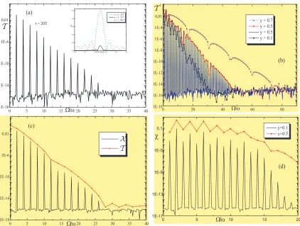
Figure 3: Fourier transform of the transmission probability for a single (a) and double (b) defect withE0= 2.0,g= 3.5,θ= 1.2,ω = 0.2. Harmonic emission spectrum for a single (c) and double

(d) defect withE0= 2.0,g= 3.5,θ= 1.2,ω= 0.2, ∆ = 6.

regions, we see that there are satellite peaks appearing near the main harmonics. They reduce their intensity whenτ is increased, such that with longer pulse length the harmonics become more and more pronounced. We also investigated that for different frequencies ω

the general structure will not change. Increasing the field amplitudeE0, simply lifts up the

whole plot without altering very much its overall structure. We support these findings in two alternative ways, either by computing directly (2.39) numerically or, more instructively, by evaluating the sums (2.42) and (2.43).

Part (b) shows the analysis for a double defect system with one defect situated at

PrHEP unesp2002

emerge in addition to the ones in (a) as harmonics, but also that we obtain much higher harmonics and the cut-off is shifted further to the ultraviolet. Furthermore, we observe a regular pattern in the enveloping function, which appears to be independent ofy. Similar patterns were observed before in the literature, as for instance in the context of atomic physics described by a Klein-Gordon formalism (see figure 2 in [44]).

Coming now to the main point of our analysis we would like to see how this structure is reflected in the harmonic spectra. The result of the evaluation of (2.51) is depicted in figure 3 parts (c) and (d). We observe a very similar spectrum as we have already computed for the Fourier transform of the transmission amplitude, which is not entirely surprising with regard to the expression (2.51). The cut-off frequencies are essentially identical. From the comparison between _X and the enveloping function for _T we deduce, that the term involving the transmission amplitude clearly dominates the spectrum.

The important general deduction from these computations is of course that harmon-ics of higher order do emerge in the emission spectrum of impurity systems, such that harmonics can be generated from solid state devices.

3. Conductance from the Kubo formula

Having characterized various features of defects, I will proceed with the main theme of the talk, that is the computation of the DC conductance. In the absence of impurities it can be obtained from the Kubo formula in the form

G(T) =₋lim

ω→0

1 2ωπ2

Z ∞

−∞

dt eiωt _hJ(t)J(0)_iT,m. (3.1)

We proposed in [1] a generalization of (3.1) in the form of (1.1). The key quantity needed for the explicit computation of (3.1) or (1.1) are the occurrence of the temperature dependent current-current correlation functions_hJ(r)J(0)_iT,m or_hJ(r)ZαJ(0)iT,m, respectively.

In the zero temperature regime two-point correlation functions can be computed in general by means of the form factor bootstrap approach [15, 16, 17]. In this approach one expands the two-point function between two local operators_Oand_O′ _{in terms of the series}

O(r)_O′(0)

T=0,m =

∞

X n=1

X µ1···µn

Z

dθ1· · ·dθn

n!(2π)n n Y i=1

e−rmicoshθi

×FO|µ1...µn

n (θ1, . . . , θn) h

FO′|µ1...µn

n (θ1, . . . , θn)

i∗

, (3.2)

where we choose xµ _{= (−ir,0). The form factors are defined as matrix elements of the}

local operator_O(~x) located at the origin between a multiparticle in-state and the vacuum,

FO|µ1...µn

n (θ1, θ2. . . , θn) :=h0|O(0)|Zµ†1(θ1)Z

†

µ2(θ2). . . Z

†

µn(θn)i. (3.3)

PrHEP unesp2002

hJ(r)ZαJ(0)i_T=0,m=

∞

X n,m=1

X µ1···µn;ν1···νm

Z _dθ

1· · ·dθndθ˜1· · ·dθ˜m

m!n!(2π)n+m F

J|µ1...µn

n (θ1. . . θn)

×DZµn(θn). . . Zµ1(θ1)|Zα|Zν1(˜θ1). . . Zνm(˜θm)

E

FJ|ν1...νm

m (˜θ1. . .θ˜m)∗e

−r

n

P

i=1

micoshθi .(3.4)

This means there are three principle steps left in order to obtain the conductance from the expression in (1.1). (a) The computation of the form factors (3.3) and the matrix elements involving the defect operator occurring in (3.4). (b) The integration in r and (c) the limit ω _→ 0. Step (a) can be performed in two alternative ways either by solving certain consistency equations for the form factors and defect matrix elements or by direct computation. For the latter we require a representation for the particle creation operators

Zµ(θ), the defect operatorZαand the local operatorO(r) which is the current in this case.

3.1 The massless limit

Remarkably when carrying out the massless limit of the above expressions, the steps (b) and (c) can be carried out generically. To perform such a limit we proceed according to the massless limit prescription as suggested originally in [45]. It consists of carrying out the limit m _→ 0 in the high energy regime. In order to do this one replaces in every rapidity dependent expression θ by θ_±σ, where an additional auxiliary parameter σ has been introduced. Thereafter one takes the limitσ_{→ ∞},m_→ 0 while keeping the quantity

ˆ

m = m/2 exp(σ) finite. For instance, carrying out this prescription for the momentum yields p±=±mˆ exp(±θ), such that one may view the model as splitted into its two chiral sectors and one can speak naturally of left (L) and right (R) movers. For the form factors in (3.4) the massless limit yields

lim

σ→∞F

O|µ1...µn

n (θ1+η1σ, . . . , θn+ηnσ) =FνO|1···µ1νn...µn(θ1, . . . , θn), (3.5)

withηi =±1 andνi =R forηi = + and νi =L forηi =−. Namely, in the massless limit

every massiven-particle form factor is mapped into 2n massless form factors. Using these expressions, performing a Wick rotation and introducing the variableE=Pn

i=1mˆieθi, we

obtain from (3.4)

hJ(r)ZαJ(0)iT=m=0=

∞

X n,m=1

X µ1···µn;ν1···νm

Z

dθ1· · ·dθndθ˜1· · ·dθ˜m

m!n!(2π)n+m F

J|µ1...µn

R1...Rn (θ1, . . . , θn) ×DZ_µR_n(θn). . . ZµR1(θ1)|Zα|Z

R

ν1(˜θ1). . . Z

R νm(˜θm)

E

FJ|ν1...νm

R1...Rm (˜θ1, . . . ,

˜

θm)∗e−irE. (3.6)

We note that for the massless prescription to work, the matrix element involving the defect

Zα can only depend on the rapidity differences, which will indeed be the case as we see

below. Performing the variable transformation θn → lnE′/mˆn−Pn_i=1mˆi/mˆneθi, we

re-write the r.h.s. of (3.6) as

∞

X n,m=1

X µ1···µn;ν1···νm

Z E

0

dE′

lnE′_/mˆ n

Z

−∞

dθ1· · ·dθn−1

n!(2π)n

∞

Z

−∞

dθ˜1· · ·dθ˜m

m!(2π)m F

J|µ1...µn

PrHEP unesp2002

R

ν1(˜θ1). . . Z

R νm(˜θm)

E

FJ|ν1...νm

R1...Rm (˜θ1, . . . ,

˜

θm)∗e−irE

′

. (3.7)

We substitute now this correlation function into the Kubo formula, shift all rapidities as

θi → θi+ lnE′/mˆn, ˜θi → θ˜i+ lnE′/mˆn, use the Lorentz invariance of the form factors2

and carry out the integration in dE′

Gα=₋lim

ω→0

ω2s−2

ˆ

m2s nπ

X µ1···µn;ν1···νm

0

Z

−∞

dθ1· · ·dθn−1

n!(2π)n

∞

Z

−∞

dθ˜1· · ·dθ˜m

m!(2π)m

1 1₋Pn−1

i=1 mˆi/mˆneθi

×DZ_µR_n(ln(1₋Xn−1

i=1 mˆi/mˆne

θi_{)). . . Z}R

µ1(θ1)|Zα|Z

R

ν1(˜θ1). . . Z

R νm(˜θm)

E

(3.8)

×FJ|µ1...µn

R1...Rn (θ1, . . . ,ln(1−

n−1

X i=1

ˆ

mi/mˆneθi))F_RJ₁|ν_...R1...ν_mm(˜θ1, . . . ,θ˜m)∗ .

We state various observations: Since the matrix element involving the defect only depends on the rapidity difference, it is not affected by the shifts. Operators with Lorentz spins= 1 play a very special role in (3.8), which makes the current operator especially distinguished. In that case the r.h.s. of (3.8) becomes independent of the frequency ω and the limit is carried out trivially. Furthermore, since the final expression has to be independent of ˆmn,

we deduce that the form factors have to be linearly dependent on ˆmn.

3.2 Realization of the defect operator

A realization ofZαcan be achieved very much in analogy to a realization of local operators,

i.e. as exponentials of bilinears in Zamolodchikov–Faddeev operators [46]. For the case of a boundary a generic model independent realization for the boundary operator B was originally proposed in [28] for the parity invariant case, i.e. R = ˜R . This proposal was generalized to the defect operator in [26] with the same restriction and for self-conjugated particles. Here we extend this realization in order to incorporate the possibility of parity breaking as well as non self-conjugated particles. A non-trivial consistency check for the validity of our proposal will be ultimately provided when exploiting it in the computation of the conductance, obtained by entirely different means as will be presented in part II. The realization we want to propose here is a direct generalization of the one presented in [26], namely

Zα =: exp[ 1

4π

Z ∞

−∞

Dα(θ)dθ] : , (3.9)

where : : denotes normal ordering and the operatorDα(θ) has the form

Dα(θ)= X

i h

K_iα(θ)Z_i†(θ)Z_¯ı†(₋θ) + ˜K_iα(θ)∗Z¯ı(−θ)Zi(θ)

+W_iα(θ)Z_i†(θ)Zi(θ) + ˜Wiα(θ)∗Zi†(−θ)Zi(−θ) i

, (3.10)

2_{Denoting bysthe Lorentz spin of the operatorOandλbeing a constant, the form factors satisfy}

FO|µ1...µn

PrHEP unesp2002

i (θ) := Rαi(iπ2 −θ), ˜Kiα(θ) := ˜Riα(iπ2 −θ), Wiα(θ) := Tiα(iπ2 −θ) and ˜Wiα(θ) :=

˜

T_iα(iπ_{2 −}θ). In comparison with [26] we have used a slightly different normalization factor, since in general we have contributions in the sum over iin (3.10) including both particles and anti-particles, as for the complex free Fermion we shall treat below. Following the arguments given in [28], the operator Dα(θ) depends on the amplitudesR(θ), T(θ), ˜R(θ)

and ˜T(θ) with their arguments shifted, as considered also in [24, 26].

3.3 Defect matrix elements

Having now a concrete generic realization of the defect (3.9), we can compute the defect matrix elements. One way of doing this is to solve a set of consistency equations which relate the lower particle matrix elements to higher particle ones, similar as in the standard form factor program [15, 16, 17]. Such kind of iterative equations were proposed in [24] for a parity invariant defect and for a real free fermionic and bosonic theory. We generalize this here and note first that the operator (3.9) becomes

lim

R,R˜→0;T,T˜→1

Zα =: exp[

1 2π

Z ∞

−∞ dθX

i

Z_i†(θ)Zi(θ) ] :, (3.11)

and the defect should act in this case as the identity operator, which fixes our normalization to _hZi(θ1)ZαZj†(θ2)i = 2π δ(θ12)δij after having contracted according to Wick’s theorem.

For two particles we find,

hZ¯ı(θ1)Zi(θ2)Zαi = πKˆiα(θ2)δ(ˆθ12), (3.12)

hZαZ_i†(θ1)Z¯ı†(θ2)i = πKˆiα(θ1)∗δ(ˆθ12), (3.13)

hZi(θ1)ZαZ_j†(θ2)i = πWˆiα(θ1)δ(θ12)δij. (3.14)

For later convenience we have introduced the functions

ˆ

K_iα(θ) = K_iα(θ) +S¯ıi(−2θ)K¯ıα(−θ) = ˜Kiα(θ) +Si¯ı(2θ) ˜K¯ıα(−θ), (3.15)

ˆ

W_iα(θ) = W_iα(θ) + ˜W_iα(₋θ)∗= ˜W_¯ıα(₋θ) +W_¯ıα(θ)∗ = ˆW_¯ıα(θ)∗, (3.16) since the Kα

i , ˜Kiα,Wiαand ˜Wiα amplitudes defined before will repeatedly appear in the

combinations (3.15), (3.16) in what follows. The latter equalities in (3.15), (3.16) follow simply from

˜

W_iα(θ) =W_¯ıα(₋θ) = ˜W_¯ıα(iπ₋θ)∗, K˜_iα(θ) =Si¯ı(2θ)K¯ıα(−θ) =Si¯ı(2θ) ˜K¯ıα(iπ−θ)∗, (3.17)

which are in turn consequences of the crossing-hermiticity properties (2.3)-(2.4). With these matrix elements we can construct the ones involving more particles recursively from

Fµm...µ1ν1...νn

α (θm. . . θ1, θ1′ . . . θ′n) := D

Zµm(θm) . . . Zµ1(θ1)ZαZ

†

ν1(θ

′

1). . . Zν†n(θ ′

n) E

=

π

m X

l=2

δµ1µ¯lδ(ˆθ1l) ˆK

α µ1(θ1)

l−1

Y p=1

Sµ1µp(θ1p)F

µm...µˇl...µ2ν1...νn

α (θm. . .θˇl. . . θ2, θ1′ . . . θ′n) (3.18)

+π

n X

l=1

δµ1νlδ(θ1−θ ′

l) ˆWµα1(θ1)

l−1

Y p=1

Sµ1νp(θ1p)F

µm...µ2ν1...νˇl...νn

PrHEP unesp2002

α (θm. . . θ1, θ′1. . . θn′) = (3.19)

π

n X

l=2

δν1ν¯lδ(ˆθ ′

1l) ˆKνα1(θ

′

1)∗

l−1

Y p=1

Sν1µp(θ1p)F

µm...µ1ν2...ˇνl...νn

α (θm. . . θ1, θ′2. . .θˇl′. . . θn′)

+π

m X l=1

δν1µlδ(θ ′

1−θl) ˆWνα1(θ

′

1)∗

l−1

Y p=1

Sν1µp(θ1p)F

µm...µˇl...µ1ν2...νn

α (θm. . .θˇl. . . θ1, θ′2. . . θn′).

Here we denoted with the check on the rapidities ˇθthe absence of the corresponding particle in the matrix element. It is clear from the expressions (3.9) and (3.10) that the only possible non-vanishing matrix elements (3.18) are those when n+m is even. Taking (3.12)-(3.14) as the initial conditions for the recursive equations (3.18)-(3.19), we can now either solve them iteratively or use (3.9) and evaluate the matrix elements directly. Closed solutions for these equations have been presented for the first time in [1].

3.4 Free Fermion wire with impurities

At this point we have to abandon the general discussion and consider a concrete theory, which for the reasons already explained we choose to be the complex free Fermion. Then the generators of the ZF-algebra Zi(θ),Z†i(θ) are just the usual creation and annihilation

operatorsai(θ), a†_i(θ).

3.4.1 Defect matrix elements

Let us now use (3.9)-(3.10) in order to evaluate matrix elements involving the defect oper-ator. In what follows, the most relevant matrix elements are those involving four particles, for which we compute

hai(θ1)a¯ı(θ2)Zαa¯ı†(θ3)a†i(θ4)i = wαi¯ı(θ1,θ2)δ(θ14)δ(θ23) +kiiα(θ1,θ4)δ(ˆθ12)δ(ˆθ34),

hai(θ1)ai(θ2)Zαa†j(θ3)a†j(θ4)i = −π2Wˆiα(θ1) ˆWiα(θ2)δ(θ13)δ(θ24)δij,

hai(θ1)ak(θ2)ai(θ3)Zαa†i(θ4)i = π2Wˆiα(θ4) ˆKiα(−θ2)

h

δ(θ14)δ(ˆθ23)−δ(ˆθ12)δ(θ34)

i

δ_i¯_k,

hai(θ1)Zαa†i(θ2)a†_k(θ3)ai†(θ4)i = π2Wˆiα(θ1) ˆKiα(−θ3)∗

h

δ(ˆθ23)δ(θ14)−δ(θ12)δ(ˆθ34)

i

δ_i¯_k,

with the abbreviations

wα_i¯ı(θ1,θ2) =π2Wˆiα(θ1) ˆW¯ıα(θ2) and kαii(θ1,θ2) =π2Kˆiα(θ1) ˆKiα(θ2)∗. (3.20)

One can now try to find solutions for alln-particle form factors either from (3.18)-(3.19) or by direct computation. For instance for the stated choice of particles involved, we compute

F_αm×(i¯ı)n×(¯ıi)(θ2m. . . θ1, θ′1. . . θ2′n) =

min(n,m)

X k=0

(₋1)m+n−2k_πn+m

(m₋k)!(n₋k)!k!k!

Z ∞

−∞

dβ1. . . dβ2n+2m

×det_A2n(β1. . . β2n;θ1′ . . . θ′2n) detA2m(β2n+1. . . β2n+2m;θ1. . . θ2m)

×

k Y p=1

ˆ

W_iα(β2p) ˆW¯ıα(β2p−1)δ(β2p−β2n+2p)δ(β2p−1−β2n+2p−1) (3.21)

×

n Y p=1+k

ˆ

K_iα(β2p)∗δ(β2p+β2p−1)

n+m Y p=1+k+n

ˆ

PrHEP unesp2002

1. . . θℓ;θ′1. . . θ′ℓ) is a rank ℓmatrix whose entries are given by

Aℓij = cos2[(i−j)π/2]δ(θi−θj′), 1≤i, j≤ℓ . (3.22)

The matrix elements are computed similarly as in [6] and references therein. Likewise we compute

F_αn×i+m×i(θn. . . θ1, θ1′ . . . θ′m) = δn,m

πn(₋1)n−1

n!

Z ∞

−∞

dβ1. . . dβn n Y k=1

ˆ

W_iα(θk)

×det_Bn(θn. . . θ1;β1. . . βn) detBn(β1. . . βn;θ1′ . . . θ′n), (3.23)

where we introduced a new rankℓmatrix_Bℓ_(θ

1. . . θℓ;θ′1. . . θℓ′) whose entries are now simply

given by

Bijℓ =δ(θi−θj′), 1≤i, j≤ℓ . (3.24)

One can verify explicitly [1] that these expressions indeed satisfy (3.18) and (3.19) .

3.4.2 Conductance in the T =m= 0 regime

It is well-known that for a free Fermion theory (also for a single complex free Fermion) the conformal U(1)-current-current correlation function is simply

hJ(r)J(0)_iT=m=0 = 1

r2. (3.25)

This expression can also be obtained by using the expansion (3.2), together with the mass-less prescription as outlined above and the expressions for the only non-vanishing form factors of the current operator in the complex free Fermion theory

F₂J|¯ıi(θ,θ˜) =₋F₂J|i¯ı(θ,θ˜) =₋iπmeθ+ ˜2θ . (3.26)

In particular, the massless limit of the previous expressions gives, according to the massless prescription,

F_RRJ|¯ıi(θ,θ˜) = ₋F_RRJ|i¯ı(θ,θ˜) =₋2πimeˆ θ+ ˜2θ , (3.27)

F_LLJ|¯ıi(θ,θ˜) = F_LRJ|¯ıi(θ,θ˜) =F_RLJ|¯ıi(θ,θ˜) =F_LLJ|i¯ı(θ,θ˜) =F_LRJ|i¯ı(θ,θ˜) =F_RLJ|i¯ı(θ,θ˜) = 0.(3.28) We these expressions we can evaluate (3.2) to (3.25). We may the insert (3.25) into (3.1) and the problem is reduced to find the Fourier transform of the functionr−2_{, which is given}

by_PR∞

−∞dr eiωrr−2 =−πω forω >0, withP denoting the principle value. This yields in the absence of a defectG(0) = 1/2π, in complete agreement with the well-known classical expression for the conductance in a wire without any impurities, see for instance [47].

For the more complicated situation ofndefects Zα1· · ·Zαnlocated in space at positions yα1. . . yαn, we compute in the zero temperature and zero mass regime

hJ(r)Zα1· · ·ZαnJ(0)iT=m=0 =

ˆ

m2

2

X i

 

∞

Z

−∞ dθ1

2 e

−2rmˆcoshθ1_Kˆα|R

i (θ1)

∞

Z

−∞ dθ2

2 Kˆ

α|R i (θ2)∗

+ ∞

Z

−∞ dθ1

2 e

θ1−rmeˆ θ1_Wˆα|R

i (θ1)

∞

Z

−∞ dθ2

2 e

θ2−rmeˆ θ2_Wˆα|R

¯

ı (θ2)



PrHEP unesp2002

cor-responding functions ˆW_iα(θ), ˆK_iα(θ), . . . For all the defects we considered, it turned out that the first contribution to the previous correlation function is actually vanishing, so that (3.29) is considerably simplified. In many of the examples, this is due to the fact that the amplitudes ˆK_iα(θ) are vanishing in the first place, as a consequence of the cross-ing relations (3.17). The vanishcross-ing of the reflection part in (3.29) also occurs in some cases as a consequence of the parity of the function ˆK_iα(θ). For instance, we find that, for the energy operator defect such function, although initially non-vanishing, satisfies

ˆ

Kα

i (θ) =−Kˆiα(−θ), such that limm→0R_−∞∞ dθKˆiα(θ)∗= 0.

We can now either use (3.29) to compute the conductance or evaluate the expression (3.8) directly in which the frequency limit is already taken, in both cases we obtain

Gα(0) = 1 2(2π)3

X i

0

Z

−∞

dθ eθwα_i¯ı|RR[ln(1₋eθ),θ]. (3.30)

There are, in addition, further generic results which can be obtained independently of the specific form of the defect. We present them at this stage and will confirm their validity below by some specific examples. Specializing to the case in which allℓdefects are of the same type and equidistantly separated, i.e. y =yα1 = · · ·= yαn. We can identify

two distinct regimes

wα_i¯ı|RR(θ1,θ2) =π2

(

ˆ

W_iα|R(θ1) ˆW_iα|R(θ2)∗ for finitey

|Wˆ_iα|R_|2 for y_→0 (3.31)

where we used in addition (3.16). Supported by our explicit examples below, we find that fory_→0 in (3.31) the amplitudes ˆW_iα|R(θ) become independent functions of the rapidity. As we have already argued above

k_iiα|RR(θ1,θ2) = 0. (3.32)

It will turn out, that the two regimes specified in (3.31) are also of a very distinct nature in the TBA context as presented in part II.

3.4.3 A wire with impurities of energy operator type

Let us exemplify the working of the above formulae with a concrete defect operator. As a simple example we choose the energy operator defect as presented in section 2.3.1. Con-sidering first a wire possessing a single defect of this type, we compute

ˆ

W_iα(θ) = 4 cosBcosh

2_θ

cosh 2θ+ cos 2B , Kˆ

α i (θ) =

2isinBsinhθ

sinB₋coshθ, w

α|RR

i¯ı (θ1,θ2) = (2πcosB)2

(3.33) withB being the effective coupling constant as defined in the caption of figure 1, such that

hJ(r)ZαJ(0)i_T=m=0=

cos2_B

r2 =⇒ G

α_{(0) =} cos2B

PrHEP unesp2002

Landauer formula (1.1).

Proceeding in the same way for a wire with two or four impurities we evaluated [1] in the regime y_≫r

hJ(r)Zα1Zα2J(0)iT=m=0=

4

1 + sin4B

r2_[cos2_(2B)−3]2, (3.35)

Gα1α2_{(0) =} 2

π

1 + sin4B

[3₋cos2_(2B)]2, (3.36)

hJ(r)Zα1Zα2Zα3Zα4J(0)iT=m=0=

1 2r2

1 + cos

8_B

[cos4_{B−2(1 + sin}2_B)2_]2

, (3.37)

Gα1α2α3α4_{(0) =} 1

4π

1 + cos

8_B

[cos4_{B−2(1 + sin}2_B)2_]2

. (3.38)

In the regimey _→0, we obtained [1]

lim

y→0hJ(r)Zα1Zα2J(0)iT=m=0 =

1

r2

cos4_B

(1 + sin2B)2 , (3.39)

lim

y→0G

α1α2_{(0) =} 1

2π

cos4_B

(1 + sin2B)2, (3.40)

lim

y→0hJ(r)Zα1Zα2Zα3Zα4J(0)iT=m=0 =

1

r2

cos4_B

cos4_{B−2(1 + sin}2_B)2

2

, (3.41)

lim

y→0G

α1α2α3α4_{(0) =} 1

2π

cos4B

cos4_{B−2(1 + sin}2_B)2

2

. (3.42)

It will turn out that we can reproduce these expressions by evaluating the Landauer formula (1.2) when computing the densities with the help of the TBA. This will now be outlined in part II together with the general conclusions concerning also this part.

Acknowledgments

We would like to thank the organizers for their kind invitation, financial support and all their efforts to make this 50th anniversary celebration of the Instituto de F´isica Te´orica possible. Furthermore we thank Carla Figueira de Morisson Faria (Max Born Institut Berlin) and Frank G¨ohmann (Universit¨at Bayreuth) for collaboration. We are grateful to the Deutsche Forschungsgemeinschaft (Sfb288) for financial support.

References

[1] O.A. Castro-Alvaredo and A. Fring, From Integrability to Conductance, Impurity Systems, hep-th/0205076.

[2] O.A. Castro-Alvaredo, A. Fring and C. Figueira de Morisson Faria, Relativistic treatment of harmonics from inpurity systems in quantum wires, cond-mat/0208128.

PrHEP unesp2002

[4] O.A. Castro-Alvaredo, A. Fring and F. G¨ohmann,On the absence of simultaneous reflection and transmission in integrable impurity systems, hep-th/0201142.

[5] O.A. Castro-Alvaredo and A. Fring, Nucl. Phys.B636[FS] (2002) 611.

[6] O.A. Castro-Alvaredo and A. Fring, Nucl. Phys.B618[FS] (2001) 437.

[7] F.P. Milliken, C.P. Umbach and R.A. Webb, Solid State. Comm. 97(1996) 309.

[8] R. Kubo, Can. J. Phys. 34 (1956) 1274.

[9] R. Kubo, M. Toda and N. Hashitsume,Statistical Physics, 2-nd ed. (Springer, Berlin, 1995).

[10] R. Landauer,IBM J. Res. Dev. 1(1957) 223;Philos. Mag. 21 (1970) 863; M. B¨uttinger,

Phys. Rev. Lett.57 (1986) 1761.

[11] F. Lesage, H. Saleur and S. Skorik,Nucl. Phys. B474 (1996) 602.

[12] P. Fendley, A.W.W. Ludwig and H. Saleur,Phys. Rev.B52(1995) 8934.

[13] P. Fendley, A.W.W. Ludwig and H. Saleur,Phys. Rev. Lett.74 (1995) 3005.

[14] C. Cohen-Tannoudji,Quantum Mechanic, (John Wiley & Sons, New York, 1977).

[15] P. Weisz,Phys. Lett. B67 (1977) 179; M. Karowski and P. Weisz,Nucl. Phys. B139(1978) 445.

[16] F.A. Smirnov,Form Factors in Completely Integrable Models of Quantum Field Theory,

Advanced Series in Mathematical Physics, Vol. 14, World Scientific, Singapore, 1992.

[17] H. Babujian, O.A. Castro-Alvaredo, A. Fring and M. Karowski,Correlation functions from form factors, an introduction, in preparation.

[18] Al.B. Zamolodchikov,Nucl. Phys.B342(1990) 695.

[19] C.N. Yang,Phys. Rev. Lett.19(1967) 1312; R.J. Baxter,Ann. Phys. 70(1972) 323.

[20] B. Schroer, T.T. Truong and P. Weisz,Phys. Lett.B63(1976) 422; M. Karowski, H.J. Thun, T.T. Truong and P. Weisz,Phys. Lett.B67(1977) 321; A.B. Zamolodchikov,JETP Lett.25 (1977) 468.

[21] I.V. Cherednik, Theor. Math. Phys.61(1984) 977.

[22] E.K. Sklyanin, J. Math. Phys.A21(1988) 2375.

[23] A. Fring and R. K¨oberle,Nucl. Phys. B421(1994) 159;Nucl. Phys. B419 [FS](1994) 647;

Int. J. of Mod. Phys. A10(1995) 739.

[24] G. Delfino, G. Mussardo and P. Simonetti,Phys. Lett.B328(1994) 123,Nucl. Phys. B432 (1994) 518.

[25] P. Federbush,Phys. Rev.121(1961) 1247;Progress of Theo. Phys.26(1961) 148;

B. Schroer, T.T. Truong and P. Weisz, Ann. of Phys. 102(1976) 156; S.N.M. Ruijsenaars,

Comm. of Math. Phys.87(1982) 181.

[26] R. Konik and A. LeClair,Phys. Rev.B58 (1998) 1872.

[27] D. Cabra and C. Na´on,Mod. Phys. Lett.A9(1994) 2107.

[28] S. Ghoshal and A.B. Zamolodchikov,Int. J. of Mod. Phys. A9(1994) 3841.

PrHEP unesp2002

[30] A. Luther and I. Peschel,Phys. Rev.B9(1974) 2911; F.D.M. Haldane,J. of Phys.C (1981) 2585; C.L. Kane and M.P.A. Fisher,Phys. Rev.B46 (1992) 15233.

[31] I. Affleck and A.W.W. Ludwig, J. Phys. A27(1994) 5375.

[32] H. Weyl,Gruppentheorie und Quantenmechanik, (Hirzel, Leipzig, 1928).

[33] W. Gordon, Zeit. f¨ur Physik40,117 (1926); D.M. Volkov,Zeit. f¨ur Physik 94,250 (1935).

[34] P.A. Franken, A.E. Hill, C.W. Peters and G. Weinrich,Phys. Rev. Lett.7(1961) 118; W. Kaiser and C. Garret,Phys. Rev. Lett.7(1961) 229.

[35] T. Brabec and F. Krausz,Rev. of Mod. Phys.72, 545 (2002).

[36] G. Sommerer,private communication (1999).

[37] M. Lenzner, J. Kr¨uger, S. Sartania, Z. Cheng, Ch. Spielmann, G. Mourou, W. Kautek, and F. Krausz,Phys. Rev. Lett.80, 4076 (1998).

[38] O. E. Alon, V. Averbukh, and N. Moiseyev,Phys. Rev. Lett.80, 3743 (1998).

[39] K.Z. Hatsagortsyan and C.H. Keitel,Phys. Rev. Lett.86, 2277 (2001);J. Phys. B35, L175 (2002).

[40] O. E. Alon, V. Averbukh, and N. Moiseyev,Phys. Rev. Lett.85, 5218 (2000); G. Ya. Slepyan, S. A. Maksimenko, V. P. Kalosha, A.V. Gusakov, and J. Herrmann,Phys. Rev. A 63, 053808 (2001).

[41] N. Hay, R. de Nalda, E. Springate, K.J. Mendham and J.P. Marangos,Phys. Rev.A 61, 053810 (2000); N. Hay, R. de Nalda, T. Halfmann, K.J. Mendham, M. B. Mason, M. Castillejo, and J.P. Marangos,Phys. Rev. A 62, 041803 (2000).

[42] V. Averbukh, O. E. Alon, and N. Moiseyev,Phys. Rev.A64, 033411 (2001).

[43] C. Itzykson and J-B. Zuber,Quantum Field Theory, (McGraw-Hill, Singapore, 1980).

[44] R. E. Wagner, Q. Su and R. Grobe,Phys. Rev.A60, 3233 (1999).

[45] Al. B. Zamolodchikov,Nucl. Phys. B358(1991) 524.

[46] M. Sato, T. Miwa and M. Jimbo,Proc. Japan Acad.53 (1977) 6; 147; 153.