4
S. Hinduja and L. Li (eds.),Proceedings of the 37th International MATADOR Conference, DOI: 10.1007/978-1-4471-4480-9_ ÓSpringer-Verlag London 2013
93 4,
4-1
Idealising mesh modelling for haptic enabled services and operands
E. Govea-Valladares1*, H. I. Medellín-Castillo1, C. Fletcher2, T. Lim2, J. Ritchie2, Xiu-Tian Yan3, Victor Arnez4 and
Ernesto Hernandez4
1 Facultad de Ingeniería, Universidad Autónoma de San Luis Potosí, S.L.P. México 2 Innovative Manufacturing Research Centre, Heriot-Watt University, Edinburgh, UK 3 Design, Manufacture & Engineering Management, University of Strathclyde, Glasgow, UK 4
Facultad de Ingeniería, Universidad Nacional Autónoma de México, D.F. México
* Corresponding author: [email protected]
Abstract. Communicating the knowledge and science of product engineering, analysis and manufacturing planning is an area of continued research driven by the digital economy. Virtual Reality (VR) is a generally accepted interactive digital platform which industry and academia have used to model engineering workspaces. Interactive services that generate a sense of immersion, particularly the sense of touch to communicate shape modelling and manipulation, is increasingly being used in applications that range from Design For Manufacturing and Assembly (DFMA) and Process Planning (PP) to medical applications such as surgical planning and training. In simulation, the natural way for solid modelling is the use of primitive geometries, and combinations of them where complex shapes are required, to create, modify or manipulate models. However, this natural way makes use of Booleans operands that require large computational times which make them inappropriate for real time VR applications. This work presents an insight on new methods for haptic shape modelling focused on Boolean operands on a polygon mesh. This is not meant as a contrast to point/mesh-editing methods, instead it is focused on idealising polygonal mesh modelling and manipulation for use with haptics. The resulting models retain a high level of geometric detail for visualisation, modelling, manipulation and haptic rendering.
Keywords: Mesh modelling, Boolean operations, Haptic rendering, Process Planning.
1. Introduction
Through the years, computer simulation has been a tool used to model real life situations by using a computer program. Traditionally, system modelling uses a mathematical model, which attempts to find analytical solutions to problems, trying to predict the behaviour of a system [1]. There are many different types of computer simulations; the common feature that they all share is the attempt to generate a sample of representative scenarios for a model and its behaviour [2].
Object modelling is a tool used in mechanical engineering to design parts [3]. Simulations play an important role in the product design process, reducing the
need for expensive prototyping and reducing the product development cost [4]. Most of commercial modelling software focuses on the visual editing, but when haptics is added the user experience through tactile engagement is superior. Precision and accuracy are desired characteristics in these systems, but it is directly dependent on the computational capabilities and the data size and complexity. The more data, the more specific becomes the model [5]. The time performance of the modelling and simulation process is a current subject under study. Current methods such as performing Boolean Operations on Polygon Meshes and implicit functions [6] are usually very slow.
This paper presents a new algorithm developed for mesh modelling and manipulation with haptics. Union, intersection and difference Boolean operands are ‘localised’ to the contact area between the two objects to speed up processing to move closer to a real-time performance. The implementation is done in VTK [7] with collision libraries of VTKBioEng [8] programmed in C++.
2. Related Work
The editing and manipulation of 3D models has seen constant research activity particularly in the area of CAD. Several techniques relevant for physics-based simulations are listed in [7]. In this work the modelling techniques for fully-automatic or semi-automatic simplification of CAD models are also characterized. In [8] a set of interactive free-form editing operators for direct manipulation of level-set models to support the creation and removal of surface detailed by operators for volumetric implicit surfaces is presented.
94 E. Govea-Valladares, H. I. Medellín-Castillo, C. Fletcher, T. Lim
modifications of the mesh models means critical problems can be solved quickly without going back to the CAD model. An algorithm that removes the intersecting faces in an n-ring neighbourhood is presented in [9]. The algorithm produces triangles whose sizes smoothly evolve according to the possibly heterogeneous sizes of the surrounding triangles. Regarding the formation of new models from primitive objects, techniques for rendering implicit surfaces using point based primitives were presented in [10]. A method for real time modelling was presented in [11], where a modelling approach using signed distance functions for objects and complex surface manipulations with immediate visual feedback was described. A new method for implicit modelling was presented in [12]. It was proposed a method to describe sharp features (edges and vertices) applying a new surface modelling representation.
In [13] Boolean operations to construct heterogeneous material objects were introduced. Boolean operations use Boolean algebra to model more complex objects. The operands of addition, subtraction and common are used in this modelling technique [14]. Boolean modelling can be readily implemented in CAD/CAE/CAM software. An algorithm to calculate intersection, union and difference was proposed in [15]. The algorithm is valid for general planar polygons based on algebraic operations to calculate the intersection between general polygons. Similarly, an algorithm for Boolean operations on polyhedral solid representations using approximate arithmetic was described in [16].
Haptic editing of 3D models was presented in [17], where the integration of Virtual Reality (VR) and Computer-Aided Design (CAD) was investigated. The proposed system made possible the intuitive and direct 3D edition of CAD objects through B-Rep modelling in CATIA and haptic aided by grid and extrude commands. Some commercial haptics 3D modellers are based on point clouds that define surfaces, essentially for applications of sculpture or artistic modelling. For example, the Splodge software of Sensable [18] or the Cre8 of Novint [20] allow 3D modelling of objects in real time.
From the literature review, it can be concluded that simulation with mesh models, haptic fast edition and manipulation of the 3D models using open source libraries and multi haptic devices, is not an area that has been explored by researchers. The purpose of this work is to model 3D mesh objects via a haptic interface and using enhanced Boolean operations. The proposed method is based on dividing the main piece (Object 1) into regions and manipulates the haptic cursor or tool (Object 2) to modify the main piece and create a new model. The aim of the method is the optimization of the processing speed when a Boolean operation is applied.
3. Methodology
Figure 1 presents the proposed methodology for haptic modelling using localised Boolean. This methodology has been implemented using C++, Visualization Toolkit libraries (VTK 5.6.1), and collision detection with VKTBioEng v5.0.1. Open Source Haptics H3D v2.1.1 is also used for haptic rendering, which in this case is carried out by the Phantom Omni from Sensable and the Falcon from Novint haptic devices. The system has been implemented in a PC with a 1.73 GHz processor, 2.0GB of RAM and Windows XP.
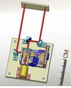
Fig. 1. Proposed Boolean localised methodology
1. - Get objects: The modelling process start with the definition of the objects in the scene (objects 1 and object 2). These objects can be created with VTK libraries (primitives) or imported from CAD systems as STL files.
2. - Divide “Object 1” in regions: In this step Object 1 is divided into smaller parts and named with an ID for identification. The algorithm divides the mesh using a filter that separates the cells of a dataset into spatially aggregated pieces using an Oriented Bounding Box (OBB) method. The division can be done by specifying the number of elements or the number of points in one area.
3. - Manipulate “Object 2”: Object 2 can be either the haptic cursor or an object being controlled with the haptic cursor. Object 1 and 2 must be in contact to allow Boolean operand being used.
4. – Identify collision: The algorithm takes only the regions of object 1 that are in contact with object 2 and creates a “polydata” variable. The data like points and elements of these regions can be extracted. The elements that are not in contact with the cursor will not be selected and will not be included in the Boolean operation procedure.
5. - Apply Boolean operation: The selected “polydata” is sent to the Boolean operation function to perform Union, Intersection or Difference.
6. - New model result: Once the Boolean operand has
Idealising mesh modelling for haptic enabled services and operands 95
Figure 2 shows an example of Object 1 after being divided into regions (colors) and the object 2 (white sphere) being the haptic cursor, before the Boolean operation.
Fig.2 Objects for the haptic modelling
4. Implementation
Four case studies were selected to test and evaluate the proposed localised approach to perform Boolean operands (intersection, union and difference) in virtual haptic modelling. For comparison purposes, Boolean operations were applied to these case studies using both, the proposed and the conventional, Boolean methods.
Case 1: Two primitive objects with regular curved surfaces (spheres) were used. Each comprises a mesh size of 780 elements. The results of each Boolean operand are shown in Fig. 3.
Case 2: In this case, a primitive cube comprising 12 triangular elements, and a sphere cursor with 780 elements were selected. The purpose of this case was to observe the behaviour of the Boolean operations when applied to an object with low resolution. Fig. 4 shows the results of the Boolean operands.
Case 3: A more complex model i.e., a gear with 1767 triangular elements was used. The objective is to test the response of the Boolean operands in areas with elements of different sizes. Fig. 5 shows the results.
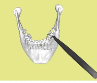
Case 4: The last case study is shown in Fig. 6. A jaw model with 9230 elements and spherical cursor were selected. The objective is to assess the performance of Boolean operands in high-resolution models of irregular geometry.
Fig. 3 Objects for the case 1: (a) source objects, (b) union, (c) intersection and (d) difference.
Fig. 4 The regular cube and cursor: (a) source objects, (b) union, (c) intersection and (d) difference.
Fig. 5 Gear and tool for the case study 3: (a) source objects, (b) union, (c) intersection and (d) difference.
Fig. 6 High resolution jaw and cursor: (a) source objects, (b) union, (c) intersection and (d) difference.
5. Results
In order to compare the time performance of the two Boolean methods, localised and conventional, processing time was measured using the CPU processor clock. Table 1 present the time performance results of the Boolean operands using the conventional approach, whilst Table 2 shows the time performance results using the proposed localised based approach. Each Boolean operand was applied ten times to each case study; the results reported in Table 1 and 2 correspond to the average values of each test.
[image:4.595.117.238.132.227.2] [image:4.595.322.510.244.342.2] [image:4.595.331.499.381.493.2] [image:4.595.80.277.578.691.2]96 E. Govea-Valladares, H. I. Medellín-Castillo, C. Fletcher, T. Lim
approach uses less data (localised data) than the conventional approach where the whole mesh is used in the Boolean operand. Since the proposed algorithm separates into parts the complete mesh of each object and uses a collision detection filter to localise and select the area of interest, the time performance is improved. By enabling discreet haptic region selection, only the elements and associated vertices of the selected regions will be affected, thus avoiding the need of procesing the whole mesh.
It can be observed that as the number of elements of the mesh models increases (more complex models), the processing time increases. The quality of the models was not affected when using the localised proposed method.
Table 1. Conventional Boolean operation, milliseconds
Haptic cursor with UNION INTERSECTION DIFFERENCE
Sphere 5.715 5.766 4.422
Cube 4.922 4.798 4.098
Gear 6.948 6.630 5.778
Jaw 7.896 7.577 7.487
Table 2. Localised Boolean operation, milliseconds
Haptic cursor with UNION INTERSECTION DIFFERENCE
Sphere 4.458 4.497 3.449
Cube 3.741 3.646 3.114
Gear 5.211 4.973 4.334
Jaw 5.685 5.455 5.391
6. Conclusions and future work
A new method to improve the time performance of Boolean operands has been proposed. The proposed method is based on a collision detection approach to localise contact areas. It has been proved that by ‘localising’ a Boolean operand on mesh models, it is possible to reduce the execution time compared with Boolean conventional operations that do not discriminate elements. It has to be mentioned that in haptic virtual reality systems, haptic rendering may be slower than Boolean operands and therefore the simulation may not be perform in real-time. Future work considers the optimization of haptic virtual reality applications using the proposed Boolean operations approach based on localised collisions.
Acknowledgements: The authors wish to thank to Consejo Nacional de Ciencia y Tecnologia (CONACyT), Universidad Autónoma de San Luis Potosi (UASLP) and Heriot-Watt University (HWU) for the invaluable support to carry out this research work.
References
[1] Oliver Rübel, Sean Ahern, E. Wes Bethel, Mark D. Biggin,
Hank Childs, Estelle Cormier-Michel, Angela DePace, Michael B. Eisen, Charless C. Fowlkes, Cameron G. R. Geddes, Hans Hagen, Bernd Hamanna, Min-Yu Huang, Soile V. E. Ker¨anen, David W. Knowles, Cris L. Luengo Hendriks, Jitendra Malik, Jeremy Meredith, Peter Messmere, Prabhat, Daniela Ushizima, Gunther H. Weber, Kesheng Wu. "Coupling visualization and data analysis for knowledge discovery from multi-dimensional scientific data", Procedia Computer 1 (2010) 1757-1764.
[2] ChaoliWang and Han-Wei Shen, "Information Theory in Scientific Visualization", Entropy 13 (2011), 254-273 [3] Junji Nomura, Kazuya Sawada. "Virtual Reality Technology
and its Industrial Applications", Annual Reviews In Control 25 (2001) 99-109
[4] Jesús David Cardona, Miguen Ángel Hidalgo, Héctor Castán, Fabio Rojas, Diego Borro, Héctor Jaramillo, "Realidad Virtual y Procesos de Manufactura" ISBN 978-958-8122-51-9. (2007) Colombia, primera edición.
[5] Atul Thakur, Ashis Gopal Banerjee, Satyandra K. Gupta. "A survey of CAD model simplification techniques for physics-based simulation applications. Computer-Aided Design 41 (2009) 65-80
[6] H. Masuda, "Topological operators and Boolean operations for complex-based nonmanifold geometric models", Computer-Aided Design 2 (1993) 119 - 129.
[7] VTK - The Visualization Toolkit, http://www.vtk.org/
[8] Vtkbioeng, http://www.bioengineering-research.com/
[9] Atul Thakur, Ashis Gopal Banerjee, Satyandra K. Gupta. "A survey of CAD model simplification techniques for physics-based simulation applications", Computer-Aided Design 41 (2009) 65-80
[10] Manolya Eyiyurekli, David Breen, "Interactive free-form level-set surface-editing operators", Computers & Graphics 34 (2010) 621-638
[11] Ruding Loua, Jean-Philippe Pernot, Alexei Mikchevitch, Philippe Vérona, "Merging enriched Finite Element triangle meshes for fast prototyping of alternate solutions in the context of industrial maintenance", Computer-Aided Design 42 (2010) 670-681
[12] Emilio Vital Brazil, Ives Macedo, Mario Costa Sousa, Luiz Velho, Luiz Henrique de Figueiredo, "Shape andtonedepictionforimplicitsurfaces", Computers & Graphics 35 (2011) 43-53
[13] Tim Reiner, Gregor Muckl, Carsten Dachsbacher, "Interactive modeling of implicit surfaces using a direct visualization approach with signed distance functions", Computers & Graphics 3 5(2011) 596-603
[14] Xinghua Song, Bert Juttler, "Modeling and 3D object reconstruction by implicitly defined surfaces with sharp features", Computers & Graphics 33 (2009) 321-330
[15] W. Sun, X. Hu, "Reasoning Boolean operation based modeling for heterogeneous objets", Computer-Aided Design 34 (2002) 481-488
[16] M. Rivero, F.R. Feito, "Boolean operations on general planar polygons", Computers & Graphics 24 (2000) 881-896 [17] J.M. Smith, N.A. Dodgson, "A topologically robust algorithm
for Boolean operations on polyhedral shapes using approximate arithmetic", Computer-Aided Design 39 (2007) 149-163
[18] P. Bourdot, T. Convard, F. Picon, M. Ammi, D. Touraine, J.-M. Vézien, "VR-CAD integration: Multimodal immersive interaction and advanced haptic paradigms for implicit edition of CAD models", Computer-Aided Design 42 (2010) 445-461
[19] Sensable, http://www.sensable.com/
4-2
Analysis of dynamic properties of a multi-stage gear system using the
flexible multi-body system modelling technique
M. Sulitka1, Z. Neusser2 and J. Veselý1
1 Research Center for Manufacturing Technology, Czech Technical University in Prague, Faculty of Mechanical
Engineering, Horská 3, Praha 2, 128 00, Czech Republic
2 Department of Mechanics, Biomechanics and Mechatronics, Czech Technical University in Prague, Faculty of
Mechanical Engineering, Technická 4, Praha 6, 166 07, Czech Republic
Abstract. The paper presents a model of a tooth gear system which allows a complex analysis of dynamic properties of the feed drive. The model, comprising a description of shaft, bearings, wheel and gearbox compliances, is assembled in state space as a coupled system of finite element models and includes a description of the stiffness of tooth contact. A measurement for verification of the proposed model is done using a single gearbox unit, as well as the entire system of a machine tool feed drive.
Keywords: Tooth gear system, Feed drive model, Machine tool
1. Introduction
The development of big machine tools with large working ranges has been intensively expanding, using rack-pinion feed drive systems increasingly as a substitute of common ball screw drives. A suitable choice of feed drive mechanism is closely linked to the interaction between the feed drive and the structure of the machine tool. An effectively optimised feed drive design can be achieved by using coupled models combining the description of feed drive and machine tool frame.
A model of a multistage tooth gear system derived from a discrete description is shown e.g. in [1]. In the present paper, a FE-based model is introduced which was developed for application in machine tool feed drive simulations. In addition to a detailed description of tooth contact and the compliance of the mechanical structure of the gear system, special attention has been paid to the contact between shaft, key and wheel.
2. Gear system model
For simulations of dynamic properties of the gear system both in frequency and time domain, a model was created which includes a description of all the important elements
of the mechanical gear system including tooth contact, shaft and wheel mechanics, bearings and gear box.
2.1. Tooth contact model
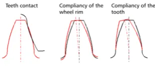
The tooth contact model assumes an ideal contact of a wheel couple. Calculation of the contact uses a modified Hertz theory [2], using the more precise parameters of tooth tilting derived in [3] and tooth bending in [4] (see Fig. 1). The resulting force is dependant on the load of the coupled gears and the rotation, with a different number of teeth in contact. Stiffness used to substitute tooth contact has been calculated as an average of instantaneous flexibilities. Dynamic properties of the tooth contact model and comparison with measurements introduces [5].
Fig. 1. Components of the compliance of tooth contact
2.2. Contact stiffness
The calculation of the stiffness of the gear contact is based on the two tooth penetration formula, in which the total penetration is dependant on the bending of both teeth caused by contact force FN, the tilting of both teeth and the transformations of the sides of the teeth in contact, according to formula 1.
[image:6.595.340.495.460.526.2]98 M. Sulitka, Zd. Neusser and J. Veselý
( 1)
Compliances gx are dependant on the line of contact,
tooth profile and material properties of the gears. Variable gcontact is described in a non-linear dependence featuring contact force FN. Therefore, the formula (1) must be solved iteratively. The stiffness of the contact is determined by dividing the contact force with total penetration.
2.3. Shaft and wheel model
An important component of the overall compliance of the gear system is represented by the system of shafts and wheels. A model was designed, enabling simulations of the operation of the gear system over time and the creation of the machine tool feed drive coupled models. An FE model, including the contact problem between shaft, key and wheel, is used for the calculation of static analysis, delivering the stiffness kCS [N/m] between a wheel W on which a tangent force F is applied and a pinion P, fixed on the circumference by the tooth contact line (Fig. 2). The shaft is fixed in bearing locations.
Fig. 2. The FE model of the shaft and wheel for a static analysis with the shaft, key and wheel contact problem.
This type of model, however, cannot be used for efficient simulations in time domain. For this reason, another FE model was created, where the shaft is united with the wheels.
Through modal decomposition, this model is transformed into state space with interface nodes i, j, k, l selected to define the force inputs and outputs of positions and rotations at points, representing the bearings and wheels (Fig. 3). This model can then be used to determine the torsion stiffness kSS [Nm/rad] between the wheel W and pinion P.
2.4. Coupled shaft and gearbox model
The coupling of the shaft models with the wheels and the gearbox is carried out in state space (Fig. 4). The coupling force between the shaft wheels 1 and 2 is determined using the total stiffness of one wheel pair
( 2)
where kt [N/m] is the contact stiffness derived from (1) and kCS [N/m] is the stiffness between the wheel and the pinion of the FE model considering the contact between shaft, key and wheel (Fig. 2). Subtracted is the element with the torsion stiffness kSS [Nm/rad], transformed to its axial representation using the wheel radius rw. On interface nodes j, k (Fig. 4), there is a torque of
( 3)
where ϕ is the rotation of the teeth and r is the appropriate gear diameter.
To determine the coupling force between the shaft and the gearbox, the stiffness values of the bearings are used.
Fig. 3. A full FE model of the shaft with wheels for export in state space (a schematic is shown on the right)
Fig. 4. Coupled model of shaft with wheels and the gearbox
3. Measuring the stiffness of the gear system
Analysis of dynamic properties of a multi-stage gear system 99
The arrangement of the test bench and tested gear system for the measurement can be seen in Fig. 5. In addition to the rotation (1) on the input shaft, rotation (2) on the output pinion and the torque on the input, deviations of the gearbox relative to the rack were also measured in directions X, Y and Z.
The gear system has been loaded by a controlled alternating torque of the servomotor, with three selected amplitude levels of the load torque. The information from rotation sensors ϕ1, ϕ2 and torque Mk on the output shaft are used to determine the overall stiffness of the gear system relative to the input as,
( 4)
where pR is the overall transmission. For the additional rotation of the pinion Δϕ2 caused by the gearbox being moved relative to the rack because of the compliance of the consoles, the following can be derived:
( 5)
where α is the angle of the sides of the rack’s teeth, β the angle of the teeth and rb is the radius of the pitch circle of the pinion.
The measurements are used to derive not only the stiffness of the entire transmission system, but also of the pinion’s mesh with the rack.
Fig. 5. Picture of gear system measuring arrangement
4. Verfification of the gear system stiffness
Hysteresis loops of the dependence of load torque on rotation are determined from the measurements, with an example of shown in Fig. 6.
In the range of used torque amplitudes, stiffness values have been determined which correspond to central lines of the hysteresis loops, with a range of 300 to 500 Nm/rad (). These points at obviously non-linear characteristic of the gear system. The simulation model evaluates linearised stiffness values, which are compared
with the measured ones in the chart in Fig. 7. Well match of the model with measurements can be seen.
Fig. 6. Measured hysteresis loops of the gear system
Fig. 7. Stiffness of the gear system relative to input. Comparison of the measurements and simulation
5. Verification of the feed drive model of the machine tool motion axis
The tested gear system is used on a large portal vertical milling machine as a feed unit of the X motion axis. For the analysis of the feed drive dynamic properties, a coupled model of the drive of X axis is created, including an FE model of the machine tool structure and a simplified two-mass substitution of the gear system mechanics. The gear system simplified model uses the value of the overall torsion stiffness determined using the detailed model described above.
5.1. Feed drive coupled model
100 M. Sulitka, Zd. Neusser and J. Veselý
model is transformed into state space. A schematic picture of the model is shown in Fig. 8.
Fig. 8. FE model of the machine and the connection with simplified models of the X-axis gear system
6. Feed drive dynamic properties
Dynamic properties of the feed drive mechanical structure are expressed with the frequency transfer ϕM/xL between the rotation of motor ϕM (encoder) and a linear movement of the column xL (linear ruler). This transfer can be evaluated with a combination of functions ϕM/Mk and xL/Mk
( 6)
A comparison between the measured and simulated characteristics is shown in a chart in Fig. 9. It can be seen that the simulation corresponds to the measurements very well, both in frequency and amplitude. It is particularly important to note the very good correspondence of the value of the first anti-resonance frequency at the first point the characteristic’s amplitude drops.
Fig. 9. Frequency transfer of the machine’s feed drive. Comparison of measurements and simulation
Regulation theory [8] has proven that setting of the position control loop gain is limited primarily by the first anti-resonance frequency. In addition to this value, however, there are also higher natural frequencies and
their oscillation amplitudes entering the feed drive control dynamics, and the model shows very good correspondence with the measurements in this area as well. The resulting model can thus be beneficially used for relevant simulations of feed drive control dynamics.
7. Summary
A detailed model of a gear system was created, including a description of the stiffness of the teeth mesh, the transmission path and the gearbox. The model is designed as a flexible multi-body system, enabling time and frequency domain simulations. The proposed shaft modelling approach also considers the contact of the shaft – key – wheel system. The model is verified with measurements on a real gear system using a specialised testing bench, determining a very good correspondence between the simulated and measured values. The gear system model is also verified on a real machine tool motion axis. The model shows a very good correspondence with the real dynamic properties of the feed drive and therefore it can well be applied in machine tool feed drive coupled models for simulating and optimizing the feed drive control dynamics.
Acknowledgements: This research has been supported by the 1M0507 grant of the Ministry of Education of the Czech Republic.
References
[1] Tanaka E, Tanaka N, Ohno k, (2001) Vibration analysis of a multi-stage gear system including drive mechanism elements. JSME Int Journal, Ser C. Mech Systems, Mach Elem Manuf, Vol. 44, No. 2
[2] Petersen D, (1989) Auswirkung der Lastverteilung auf die Zahnfusstragfähigkeit von hoch überdeckenden Strinradpaarungen. Dissertation, Hamburg, Germany
[3] Sainsot P, Velex P. (2004) Contribution of Gear Body to Tooth Deflections - A New Bi-dimensional Analytical Formula. Journal of Mechanical Design, Vol. 126: 748-752 [4] Weber C, Banaschek K, (1953) Formänderung und
Profilrücknahme bei Gerad-und Schrägverzahnten Rädern. Heft 11, F. Vieweg und Sohn, Braunschweig, Germany. [5] Neusser Z, Sopouch M, Schaffner T, Priebsch H-H, (2010)
Multi-body Dynamics Based Gear Mesh Models for Prediction of Gear Dynamics and Transmission Error. SAE konference, Detroit, USA.
[6] Sulitka M, Strakoš P, (2007) Complex model of a real machine tool feed drive axis with ball screw. Conference VIDA 2007; Poznan, Poland,
[7] Vesely J, Sulitka, M, (2008) Machine Tool Virtual Model. International Congress MATAR 2008, Part 1: Drives & Control, Design, Models & Simulation; Prague; Czech Republic;
4-3
An efficient offline method for determining the thermally sensitive points of
a machine tool structure
N. S. Mian, S. Fletcher, A. P. Longstaff and A. Myers University of Huddersfield, Queensgate, HD1 3DH, UK
Abstract. Whether from internal sources or arising from environmental sources, thermal error in most machine tools is inexorable. Out of several thermal error control methods, electronic compensation can be an easy-to-implement and cost effective solution. However, analytically locating the optimal thermally sensitive points within the machine structure for compensation have been a challenging task. This is especially true when complex structural deformations arising from the heat generated internally as well as long term environmental temperature fluctuations can only be controlled with a limited number of temperature inputs. This paper presents some case study results confirming the sensitivity to sensor location and a new efficient offline method for determining localized thermally sensitive points within the machine structure using finite element method (FEA) and Matlab software. Compared to the empirical and complex analytical methods, this software based method allows efficient and rapid optimization for detecting the most effective location(s) including practicality of installation. These sensitive points will contribute to the development and enhancement of new and existing thermal error compensation models respectively by updating them with the location information. The method is shown to provide significant benefits in the correlation of a simple thermal control model and comments are made on the efficiency with which this method could be practically applied.
Keywords: Finite element analysis, FEA, Matlab, Thermal error, Thermal error compensation, Thermally sensitive locations.
1. Introduction
Thermal errors have been identified as a major contributor to the overall volumetric error of a machine tool, in many cases up to 70% [1]. Several techniques based on analytical, empirical and numerical methods have been established to control the effect of thermal errors. These techniques are widely used and applied with a basic ideology to establish a thermal model based on relationships between the measured temperature of the machine from various locations, used as temperature inputs and the displacement at the tool [2]. The temperature inputs however in some cases may be difficult to identify if propagation of the temperature gradients is complex due to the combined effect of internal and external heat sources and perhaps due to the
complexity of the machine structure. These ambiguities therefore add complexities to identify sensitive locations within the structure and stand out to be a challenging task with a limited number of temperature inputs. It has been observed that the performance of the conventional empirical and statistical approaches such as Artificial Neural Network (ANN) and Linear Regression [3, 4] heavily rely on the data from sensitive location within the machine structure for effective and robust thermal compensation such as varying environmental conditions. Kang et al. [5] used a hybrid model consisting of regression and NN techniques to estimate thermal deformation in a machine tool. The total of 28 temperature sensors were placed on (18) and around (10) the machine to acquire internal heating and environmental data. The training time for the model was 3 hours. Yang et al. [6] tested INDEX-G200 turning centre to model thermal errors. Temperature variables were selected using engineering judgement as temperature sensors were placed on or near the possible heat sources and Multiple Linear Regression technique was used to model thermal errors. Training time for the thermal model however was not mentioned. Krulewich [7] used the Gaussian integration method using polynomial fit to identify the optimum thermal points on the machine spindle. The spindle was put through heating and cooling cycles providing 3.5 hours of training data to locate three optimum measurement points where the results correlated to 96%. The author compared this method with a statistical technique and found that the Gaussian integration method requires significantly less training data.
It has been observed that a significant amount of data is generally required to identify sensor locations and train models which inevitably require machine downtime; therefore, such methodologies can be impractical for general application. It is also the fact that machine structures are sensitive to environmental changes which means that the training data acquired in the first instance may not respond well to the new conditions and therefore a new set of training data may be required [7]. This paper
102 N.S. Mian, S. Fletcher, A.P. Longstaff and A. Myers
presents an offline technique based on FEA. The technique provides the ability to identify optimised sensitive locations within the machine structure offline for any set of data either from internal heating or external environmental conditions. Being software based, using the Graphical User Interface (GUI) of the FEA software, this technique integrates the visual aspect to aid reviewing the location of the sensitive areas and the practicality for sensor installations. The application of this technique requires minimal machine downtime as any set of the measured thermal conditions can be assessed offline to obtain the thermal behaviour of the machine. This means that new sensitive areas inside the machine structure may be located according to the new thermal conditions. Satisfactory correlations between the measured and the FEA simulated results are a pre-requisite to the application of this technique. In this paper, this technique is applied on the results from simulation case study previously conducted.
2. Case Study
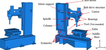
[image:11.595.91.267.463.547.2]This study was conducted on a 3 axis Vertical Machining Centre (VMC) located on the shop floor with uncontrolled environmental temperature. The FEA model of machine was created in Abaqus/Standard 6.7-1 software [10] using manufacturer provided engineering drawings. Fig. 1 shows the generated CAD model of the machine. The model of the machine was simplified by cutting into half because of the symmetry in the X axis direction and complex structures such as fillets and chamfers were simplified and represented using simple corners to avoid complexity of meshing and nodes.
Fig. 1. Generated CAD model of the machine assembly
Mian et al. [8, 9] conducted tests to exploit the thermal behaviour of the VMC when subjected to the spindle heating and varying environmental conditions. Mian et al. [8, 9] proposed a technique in which only one short term data set obtained during one hour internal heating is required to obtain thermal parameters and simulate the heat transfer within structures. This short term data set is used to create the FEA thermal model to simulate the machine for a variety of real world testing regimes. The results showed good correlation between the experimental results and the FEA simulated results typically between 70% and 80%. Mian et al. [9] also conducted environmental tests where the machine was tested for
three continuous days in two seasons (winter and summer). The aim was to achieve good correlation in results from one season test and validate the methodology with good correlation results in different environmental conditions i.e. in a different season. Both tests successfully validated the FEA environmental thermal model with good correlations typically above 60%. This technique in effect can remarkably reduce the machine downtime by creating the CAD model of the machine in the FEA software and simulate it to create an environmental thermal model that is able to simulate the effect of any set of varying environmental conditions.
This method therefore provides a platform to use FEA modelling as an offline tool to determine not only machine behaviour, but also help with the development of compensation models by determining the location of sensitive nodes/areas. The case study by Mian et al. [8, 9] was therefore used for differentiating between areas sensitive to internal heating and environmental temperature fluctuations.
The remainder of the paper details a method and the developed software for the offline assessment of the FEA data and help determine the temperature-displacement sensitive nodes based on search parameters and their physical locations within the FE model. The information can be used to retrofit sensors for compensation; however there can be practical limitations to their attachment.
3. Nodal data extraction
Abaqus simulation software provides the facility to extract surface and sub-surface nodal data within the FEA model. Since the model has to be meshed for FEA analysis, nodes from the mesh can be used to represent individual points on the structure. Therefore, using this facility, the nodal data was extracted to find nodes of interest. The predicted error is obtained as the difference in displacement between a node on the table and a node on the tool. In this case the dependant parameters are slope and hysteresis.
An efficient offline method for determining the thermally 103
3.1. Matlab program routines
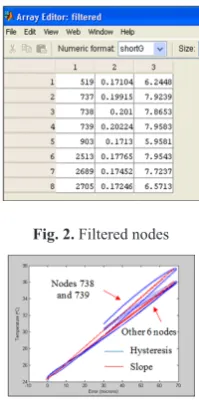
The function imports the nodal data from the FEA software and extracts the error between the tool and workpiece in each direction, and the temperature of all the nodes. Then it calculates the slope (°C/μm) using a linear least square fit and hysteresis (μm), using deviation from the straight line, for all nodes. These are compared against a predefined set of ranges to filter out the best nodes. The range may be set based on the resolution of the temperature sensors and required accuracy for compensation. There can be thousands of nodes depending on the mesh density of the machine model. If no nodes are found then the range must be widened. The nodes are filtered for slope and hysteresis separately to maintain flexibility so that different nodes can be used for different jobs, not always both. The final node numbers satisfying both filters are then used to locate their positions in the CAD model of the relevant structure. Fig.
[image:12.595.366.466.74.278.2]1 shows the function calls where comparison takes place using a specified range, in this case the range for the slope sensitivity is from 0.17 °C/μm (min) to 0.20 °C/μm (max) and 5.44 μm (min) to 8 μm (max) for the hysteresis. The first and second lines filter out node numbers for the slope sensitivity and hysteresis respectively using the range. The third line is then used to match node numbers in both arrays and obtain the matched nodes numbers. Fig. 2 shows the Matlab array editor displaying 8 nodes filtered out from the total of 4113 from the carrier (Fig. 5) structure mesh. The first column shows node number, the second column shows slope sensitivities and the third column shows the hysteresis values. These 8 nodes have shown to have the highest slope sensitivities (Fig. 3) and the lowest hysteresis values and will effectively be used to place permanent temperature sensors for use in error compensation systems. It can also be observed that nodes 738 and 739 possess the highest slope sensitivity among the other filtered nodes and a slightly higher hysteresis values relative to the other filtered nodes, however an agreement can be obtained to prioritize the selection of nodes that were located at the surface for practical installation of temperature sensors. This priority may not be the case if slope sensitivities and hysteresis values are significant at node positions inside the structure.
Fig. 1. Part of Matlab program code for assigning range
Fig. 2. Filtered nodes
Fig. 3. Slope and hysteresis plot
4. Internal heating test – Carrier sensitivity against the Y axis and Z axis displacement
[image:12.595.331.511.432.538.2]Since the carrier holds the spindle in place, it is the most affected structure as the heat from the spindle flows directly into it. Therefore, this structure was analysed to locate the temperature-displacement sensitive nodes for internal heating. Fig. 4 shows the visual representation of the simulated deformation of the machine.
Fig. 4. Simulated visual representation of deformation of the machine due to internal heating
Fig. 5 shows the best surface nodes found using the Matlab search routine. Other visible nodes are inside the structure.
Best surface node in Z axis
Best surface nodes in Y axis
Fig. 5. Nodes sensitive to spindle heating on the carrier Range
Minimum hysteresis
sensitivity Maximum slope sensitivity
Original machine structure
[image:12.595.337.482.614.686.2]104 N.S. Mian, S. Fletcher, A.P. Longstaff and A. Myers
5. Validations
Using the similar approach shown in section 3.1, the best identified surface node (Fig. 6) was checked which give the sensitivity of 0.20°C / µm and hysteresis of 7µm. This linear fit gives a simple model for the Y axis of 5Δtint -
106.5. This was applied to measured temperature data from a sensor fitted to the machine surface close to the identified node position, with correlation to measured displacement of 84% as shown in Fig.7.
Fig. 6. Validation of the FEA model against measured error due to internal heating
5.1. Environmental sensitive nodes inside the full machine structure
Using the similar procedure the nodes sensitive to the varying environmental conditions, including different seasons, were found in the machine structure. During this preliminary work, each structure was analysed individually for efficiency to locate sensitive nodes with the higher slope and lowest hysteresis approach. Further to consider the full machine structure as one component to locate the set of sensitive nodes. Fig. 7 shows the full machine FEA model with highlighted environmental sensitive nodes individually located on components.
6. Conclusions
It has been observed that the simulation of thermal behaviour of complex machine structures using FEA can provide a solid platform for offline assessment of the machine error and model identification. FEA results from previously conducted case studies were used to locate nodes in the structural elements of a 3 axis VMC that were sensitive to temperature change and movement of the machine structure in Y and Z axes. Matlab functions were used to manipulate the extracted data from the FEA software, calculate the hysteresis and slope for any given node and filter out the best node locations by using a range of highest slope sensitivity and lowest hysteresis value. The location of the filtered nodes were analysed using the Abaqus GUI. The priority is given to surface nodes rather than the internal nodes for practical temperature sensor installation on the machine. The validation result showed the predicted sensitive nodal location correlated to better than 84%. By determining the best linear relationships, simple models are available
and compatible with the common thermal compensation methods available in most modern NC controllers.
Column node sensitive in
Y axis
Base node sensitive in Z
axis sensitive in Y axisBase node Table node sensitive in Z axis
Table node sensitive in Y axis Carrier node sensitive in Y axis Column node
sensitive in Z axis
Carrier node sensitive in Z axis
Fig. 7. Environmental sensitive nodes within the full machine
Acknowledgements: The authors gratefully acknowledge the UK’s Engineering and Physical Sciences Research Council (EPSRC) funding of the Centre for Advanced Metrology under its innovative manufacturing program.
References
[1] Bryan, J., International Status of Thermal Error Research (1990). CIRP Annals - Manufacturing Technology, 1990. 39(2): p. 645-656.
[2] Chen, J.S. and G. Chiou, Quick testing and modeling of thermally-induced errors of CNC machine tools. International Journal of Machine Tools and Manufacture, 1995. 35(7): p. 1063-1074.
[3] Tseng, P.C., A real-time thermal inaccuracy compensation method on a machining centre. International Journal of Advanced Manufacturing Technology, 1997. 13(3): p. 182-190.
[4] Yang, S., J. Yuan, and J. Ni, The improvement of thermal error modeling and compensation on machine tools by CMAC neural network. International Journal of Machine Tools and Manufacture, 1996. 36(4): p. 527-537.
[5] J Yang, J.G., et al., Testing, variable selecting and modeling of thermal errors on an INDEX-G200 turning center. International Journal of Advanced Manufacturing Technology, 2005. 26(7-8): p. 814-818.
[6] Kang, Y., et al., Estimation of thermal deformation in machine tools using the hybrid autoregressive moving-average - Neural network model. Proceedings of the Institution of Mechanical Engineers, Part B: Journal of Engineering Manufacture, 2006. 220(8): p. 1317-1323 [7] Debra A, Krulewich., Temperature integration model and
measurement point selection for thermally induced machine tool errors. Mechatronics, 1998. 8(4): p. 395-412.
[8] Mian, N.S., et al., Efficient thermal error prediction in a machine tool using finite element analysis. Measurement Science and Technology, 2011. 22(8): p. 085107.
[9] Mian, N, Fletcher, S, Longstaff, A.P., Myers, A and Pislaru, C, Efficient offline thermal error modelling strategy for accurate thermal behaviour assessment of the machine tool. In: Proceedings of Computing and Engineering Annual Researchers' Conference 2009: CEARC’09. University of Huddersfield, Huddersfield, pp. 26-32. ISBN 9781862180857.
4-4
Development of an Abbé Error compensator for NC machine tools
K. C. Fan, T. H. Wang, C. H. Wang and H. M. Chen
Department of Mechanical Engineering, National Taiwan University, Taiwan, ROC
Abstract. Abbé error is the inherent systematic error in all numerically controlled (NC) machine tools due to the fact thatthe scale measuring axis is not in line with the cutting axis. Any angular error of the moving stage will result in the position offset from the commanded cutting point. In this report, a new concept of multi-sensor feedback system of the NC controller is presented. A miniature three-axis angular sensor is embedded in each axis to real-time detect angular errors of the moving stage. An error compensator is developed to calculate induced volumetric errors and fed back to the NC controller. This feedback error compensation system automatically corrects the Abbé error of the machine tool. Experiments show that the volumetric accuracy can be improved significantly by employing the proposed Abbe error compensator.
Keywords: machine tools, Abbé error, multi-sensor feedback, volumetric error compensation.
1. Introduction
Abbé error is the inherent systematic error in all numerically controlled (NC) machine tools. the Abbé principle is regarded as the first principle in the design of precision positioning stages, machine tools, and measuring instruments [1]. It defines that the measuring apparatus is to be arranged in such a way that the distance to be measured is a straight-line extension of the graduation used as a scale. Bryan further made a generalized interpretation with that if the Abbé principle is not possible in the system design, either the slideway that transfer the displacement must be free of angular motion or the angular motion data must be obtained to compensate the Abbé error by software [2, 3].
Nowadays, most commercial machine tools and CMMs still cannot comply with Abbé principle because the scale axis is always parallel to the moving axis. A very popular way to improve the accuracy is to store the positioning or volumetric errors through prior measurement or calibration process and then compensate for the error budget with software, which is called the feed-forward compensation [4, 5]. It, however, can only compensate for the mean systematic errors. The angular errors are subject to the time-varied temperature changes. It is known that if the Abbé principle is not possible in the system design, one effective method is to obtain the
real time angular data and compensate for the volumetric error in real-time [6].
Techniques of non-contact angle measurement find applications in many fields. Autocollimators are commonly used optical tools for straightness calibration [7]. Some multi-degree-of-freedom (MDOF) measurement systems have been developed for measuring angular and straightness errors of precision machines but did not feed back to the controller for real-time compensation [8-10]. Laser interferometer, with its superiority in accuracy and resolution, also has been applied for angle measurement [11, 12]. By counting interference fringes the tiny displacement of objective point can be detected and converted into angle value. The resolution can be improved by techniques of phase subdivision to very fine [13]. The author’s group has developed a miniature interferometer system for holographic gratings with good performance in measuring uncertainty and signal quality [14].
This paper presents a new approach for real-time Abbé error compensation on the machine tools by hardware. A low-cost three-angle sensor is developed that can embed in each axis of the machine tool. With an appropriate interface connection with the NC controller, this system can successfully compensate for the Abbé error during machine running condition. Experimental results show that the positioning errors within the working volume can be significantly reduced.
2. Abbé error in machine tool
Current NC controller in the machine tool feeds back the scale reading position, which is offset from the real commanded position, as shown in Fig. 1. The straightness error of the slideway will cause angular motion (θ) of the moving table yielding inevitable positioning error (δ) at the cutting point, which is offset from the scale reading position by L.
δ
=Ltan( )θ
(1)106 K.C. Fan, T.H. Wang, C.H. Wang, H.M. Chen
From the 3D point of view, the moving table has three angular errors, namely pitch, yaw, and roll. Any of these angles will induce positioning errors at the cutting points in three dimensions, as shown in Fig. 2. The corresponding errors can be expressed by the following equation.
X Z Y Y Z
Y Z X X Z
Z Y X X Y
L
L
L
L
L
L
δ
θ
θ
δ
θ
θ
δ
θ
θ
− ⋅ + ⋅
=
⋅
−
⋅
− ⋅
+
⋅
[image:15.595.69.284.154.532.2](2)
[image:15.595.356.477.351.494.2]Fig. 1. Abbé error in 1D stage
Fig. 2. Abbé error in the 3D space of a linear stage
It is known that to eliminate δ by letting L or θ zero is impossible. The only way is to compensate for the positioning errors by sensing both L and θ and correct the cutting position through the controller. The design of low cost three-angle sensor is necessary.
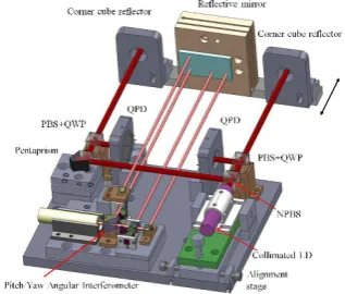
3. Principle of miniature angular interferometer
The optical structure of the proposed system is shown in Fig. 3. The principle is based on the classic model of Michelson interferometer. The approximately linear polarized beam from the laser diode is split by the polarization beam splitter PBS1. The P-polarized beam
passes through and the S-polarized beam is reflected to the left. With careful rotation of the PBS1 these two beams will have equal intensity. Then, the reflective mirrors M1, M2 and M3 guide these two beams to the object mirror in parallel and equal path distance. When the object mirror has an angle displacement, the change of the optical path difference will cause interference of two returned beams after joining together, which can be converted into corresponding angle value. After passing through the quarter waveplate Q1 twice, the left-arm beam will be converted into P-polarized beam and pass through PBS1. The right-arm beam has the similar feature. This design is to avoid the beam returning back to the laser diode. After passing through Q3 the left-arm beam and arm beam will be converted into right-circularly and left-right-circularly polarized beams, respectively. The NPBS divides both beams into two split beams of equal intensity. These four beams will be separated by 0–90–180–270 degrees by PBS2 and PBS3 (set fast axis to 45 degrees) and interfere with each other. Four photo detectors (PD) will convert the beam intensity to corresponding current. A proper sinusoidal signal processing circuit can reach 0.1 arc-sec resolution. Fig. 4 is the compact size of this developed yaw angle sensor.
Fig. 3. Optical configuration of angle interferometer
[image:15.595.355.479.532.686.2]Development of an Abb error compensator for NC machine tools 107
4. The Three-angle Sensor
[image:16.595.304.493.253.511.2]A miniature three-angle sensor has been developed for this purpose, as shown the schematic diagram in Fig. 5. One laser diode splits the beam into two angle interferometer modules set in orthogonal directions, one for the yaw and another for the pitch measurements. The second laser diode also splits the beams to two parallel paths and each one is reflected by a corner cube reflector (CCR) and collected by a quadrant detector. The relative up and down straightness motions of two CCRs reflect the roll angle motion of the stage. Fig. 6 shows the physical size (about 160 mmx 130 mm) of the developed three-angle sensor on one axis of the machine tool. After calibration, the pitch and yaw sensors can reach ±0.3 sec accuracy for the range of ±100 sec, and for roll angle it is ±1 sec accuracy for the range of ±150 sec. These performances are good enough for machine tool use.
[image:16.595.99.258.301.436.2]Fig. 5. The integrated structure of a three-angle sensor
Fig. 6. Photo of a three-angle sensor on the machine tool
5. Experiments
Fig. 7 shows the schematic diagram of mounting the three-angle sensor module on each axis of the machine tool and the integration with the PC-based NC controller. A microprocessor that processes the angle signals and calculates Eq. (2) is called the Abbé error compensator, which can dynamically acquire the current three coordinate positions from the NC controller and, after processing, send the compensated command into the
controller. By this way, the cutting point can be automatically adjusted in real-time with the amount of Abbé errors in space.
A test trial has been carried out on a small NC machine tool. The experimental setup is shown in Fig. 7 for the X-axis motion. A laser interferometer of HP5529 was amounted at different Z heights of the spindle head as a calibration reference. Same procedure can also be conducted for the Y-motion. Figures 8 and 9 show the comparison of positioning errors with and without the Abbé error compensation in X- and Y-axis respectively. The kinematic error of the table can be regarded as a rigid body motion. It is clearly seen that the positioning errors can be significantly reduced when the Abbé error compensation scheme is activated at any position.
[image:16.595.111.247.463.565.2]Fig. 7. Experimental setup for positioning test
Fig. 8. Experimental results of X-positioning error calibration.
Fig. 9. Results of Y-positioning error calibration
[image:16.595.332.515.542.646.2]108 K.C. Fan, T.H. Wang, C.H. Wang, H.M. Chen
6. Conclusions
In this paper, a developed low cost miniature three-angle sensor module is presented. It is able to embed in the machine tool structure and compensate for the positioning errors within the working zone. The developed Abbé error compensator can be equipped to any machine tool for real-time Abbé error compensation. Experimental results show the effectiveness of this system. Since this is a real-time feedback error compensation system, it can realize the goal of time-variant volumetric error compensation on any NC machine tool.
References
[1] Abbé E, (1890) Meßapparate für physiker. Zeitschrift für Instrumentenkunde 10: 446–448
[2] Bryan JB, (1979) The Abbé principle revisit: An updated interpretation. Precision Engineering 1: 129–132
[3] Wright DA and Bryan JB, (1979) Letters. Precision Engineering 2: p2.
[4] Ni J and Wu SM, (1993) An on-line measurement technique for machine volumetric error compensation. ASME J of Engineering for Industry 115: 85–92.
[5] Okafor AC, Ertekin YM, (2000) Derivation of machine tool error models and error compensation procedure for three axes vertical machining center using rigid body kinematics. International J of machine Tools & Manufacture 40: 1199– 1213.
[6] Huang PH and Ni J, (1995) On-line error compensation of coordinate measuring machines. International J of Machine Tools 35: 725–738.
[7] Yoder PR, Schlesinger JE, and Chickvary JL, (1975) Active annular beam laser autocollimator system. Applied Optics 14: 1890–1895.
[8] Fan KC, Chen MJ and Huang WM, (1998) A six-degree-of-freedom measurement system for the motion accuracy of linear stages. Int. J. of Machine Tools & Manufacture 38: 155–164.
[9] Liu CH, Hsu CC, Jywe WY and Hsu TH, (2005) Development of a laser-based high-precision six-degrees-of freedom motion errors measuring system for linear stage. Review of Scientific Instruments 76: 055110-1–055110-6. [10] Gao W, Arai Y, Shibuya A, Kiyono S and Park CH, (2006)
Measurement of multi-degree-of-freedom error motions of a precision linear air-bearing stage. Precision Engineering 30: 96–103.
[11] Jablonski ER, (1986) Interferometric measurement of angles. Measurement 4 (4): 148-153.
[12] Ikram M and Hussain G, (1999) Michelson interferometer for precision angle measurement. Applied Optics 38: 113–120. [13] Brich KP, (1990) Optical fringe subdivision with nanometric
accuracy. Precision Engineering 12: 195-198.
4-5
A novel haptic model and environment for maxillofacial surgical operation
planning and manipulation
X-T Yan1, E Hernandez2, V Arnez2, E Govea3, T Lim4, Y Li1, J Corney1 and V Villela2 1Design, Manufacture & Engineering Management, University of Strathclyde, Glasgow, UK 2
Facultad de Ingeniería, Universidad Nacional Autónoma de México, D.F. México
3 Centro de Investigación y Estudios de Posgrado, Facultad de Ingeniería, Universidad Autónoma de San Luis Potosí,
S.L.P. México
4 Innovative Manufacturing Research Centre, Heriot-Watt University, Edinburgh, UK
Abstract. This paper presents a practical method and a new haptic model to support manipulations of bones and their segments during the planning of a surgical operation in a virtual environment using a haptic interface. To perform an effective dental surgery it is important to have all the operation related information of the patient available beforehand in order to plan the operation and avoid any complications. A haptic interface with a virtual and accurate patient model to support the planning of bone cuts is therefore critical, useful and necessary for the surgeons. The system proposed uses DICOM images taken from a digital tomography scanner and creates a mesh model of the filtered skull, from which the jaw bone can be isolated for further use. A novel solution for cutting the bones has been developed and it uses the haptic tool to determine and define the bone-cutting plane in the bone, and this new approach creates three new meshes of the original model. Using this approach the computational power is optimized and a real time feedback can be achieved during all bone manipulations. During the movement of the mesh cutting, a novel friction profile is predefined in the haptical system to simulate the force feedback feel of different densities in the bone.
Keywords: Haptic surgical planning, mesh model, bone cutting, DICOM images, process planning, friction model.
1. Introduction
During the last decade there have been several research efforts [1-4] to achieve an interface with which the user could do practices in medicine, without the need to use a human body or animal, all inmersed in a virtual environment. In order to enhance this work a haptic property is added, having said that, many researchers have been driven to develop a system that is realistic in both feeling and visual [5-6].
The increasing research interests into tactile displays and haptic feedback systems to augment virtual reality in the last five years have led to trial haptic devices that aid the training of hand-based skills in applications such as
medical training. There are commercially available devices such as the PHANToM by Sensable Technologies [7] and the Cyberglove by Immersion Inc. [8]. Research has already been conducted into simulating jaws, body parts and so on using such devices. However, these devices are designed to give haptic feedback for relatively lower resolution and large surface areas to give the impression of interacting with large volumes, and cannot provide the correct force feedback. The devices were therefore found to be unsuitable for haptic feedback. In addition, the extremely high cost of these devices makes them inaccessible to mass medical training.
This paper describes findings of research work undertaken in collaboration among authors from several institutions on the application of haptic technology and development of a haptic model for maxillofacial operation planning and training. This haptic environment has been used in conjunction with medical images obtained from computerized tomography scanners, looking to train medical doctors and in some cases to plan surgical operations.
The solutions in physics are implemented in an environment that generates a friction and stiffness on the body, both forces have been studied and reported several times, but the solutions in visual environments are mainly going in two ways, one using polygonal meshes and the other using voxels. Both types of solutions have their own difficulties when interacting with the physics solutions. When using meshes, the computational power tends to be exhaustive when detecting collisions and doing a cutting function, but the resolution can be good enough for medical purposes. In more recent work, the use of voxels is becoming more present since they need less computational power to handle cutting functions and detecting collisions, but in the counter part they are not very accurate for some particular applications.
110 X-T Yan, E Hernandez, V Arnez, E Govea, T Lim, Y Li, J Corney and V Villela
The need to develop a method that achieves a precise cutting function with a computational power enough to maintain a haptic rendering is paramount at this stage of the study. It is because of this that the objective of the present paper is to design and develop a haptic interface that uses few computational resources, allowing having a real-time feedback and a good resolution when cutting the model.
2. Image capture of a subject’s head
2.1. DICOM images processing
CT scans are commonly used to scan a patient and capture the tissues, bone void etc in many slices of images. A CT scan model is provided for this research to develop a haptic model for geometry representation of a patient head. At this first stage the images captured by the CT are counted, and these images are in an unrecognizable format for the computer without the specific software. They consist in a series of files inside a folder where each file contains the information that describes the material density of a transversal section of the patient’s body: in other words, is the radiography taken of a specific plane of the patient, in this manner, by joining all the images together a 3D image of the body can be reconstructed.
To achieve this image compilation and the representation as a volumetric body, the VTK (Visualization ToolKit) libraries were used in this research. These libraries have functions that allow an easy management of the images and the graphic resources of the computer, and they are built on top of the open software OpenGL, which is the standard in graphics management for various operating systems such as Microsoft Windows.
To compile a series of images stored in the folder, it is essential to develop an appropriate algorithm to construct the three-dimensional model of the patient. The algorithm of the program to read the DICOM images (images taken from the CT) is as follows:
• Create a VTK variable to read DICOM files. Load the address where the images are allocated in the computer memory.
• Make sure that the model is in three dimensions. • Apply a reduction factor.
• Create a variable to allocate the volume information.
• Add the properties of colour and volume opacity. • Apply filters to the variable that contains the
information of the DICOM images. These filters are: contour filter, triangle filter to generate the mesh, decimation, cleaning the mesh of non-connected points.
• Generate a STL file.
• Draw the volume on screen to visualize the result.
• End program.
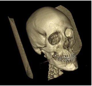
[image:19.595.337.498.187.336.2]Codifying the above algorithm it is possible for the program to create a window to visualize the DICOM images and a file with in STL format. The generated image represents a skull for this example, and the program adds some properties to make it look like bone shown in Fig. 1.
Fig. 1. DICOM images representation.
2.2. Partition the jaw part from the head model
As the research is to focus on the support of surgical maxillofacial operations, it is more efficient to extract the jaw model only in order to minimise the computational burden for haptic modelling. For this phase no filter generated by computational algorithms is needed, the reason is that an image processing based on the human anatomy is required, and to do so the human knowledge is needed. Because of this, the software MeshLab is used, which in essence reads the STL file and shows it on the screen. In addition, it gives the freedom to edit the mesh file manually: that is, it supports the manipulation of the geometry by selecting the points and faces with the mouse. This provides freedom for more accurate and smooth operations of the model if necessary.
Since the jaw is required to be isolated from the skull (Fig. 2), a computational tool could be used to save time and effort in some circumstances. This tool is a filter implemented in VTK that allows to delete from the mesh all of the points and faces that have no connection with the biggest continuous volume in the file. This tool can be executed as many times as needed during this phase. The algorithm to apply this filter is as follows:
• Create a VTK variable to read the STL file. To load the address of the file in the variable.
• Apply the connexion filter to the previous variable.
• Create a STL file with the resulting information after the filter.
A novel haptic model and environment for maxillofacial surgical 111
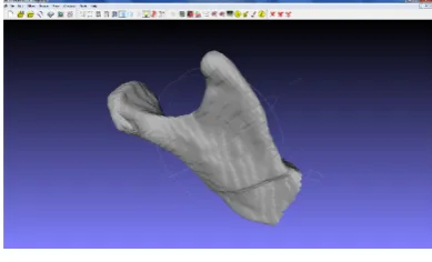
Fig. 2. Jaw obtained.
For the purpose of demonstration of concept and for future tests, a portion (Fig. 3) of the previous mesh is selected and used, and it is the right side of the bone.
Fig. 3. Portion of the jaw.
3. Haptic model
3.1. Preparing the cut
This third phase is the main objective of the work in this project, because it involves adding the cutting function to a haptic interface. All the load of the work goes directly over C++ using VTK libraries.
The algorithm for the cut is as follows:
• Create a VTK variable to read STL files. To load the address of the STL file to use.
• Call a cutting function giving the Cartesian coordinates of the position where the cut is required.
• Inside the cutting function, use a VTK function to extract geometries from de VTK variable that contains the mesh information.
• Create a widget using the data received in the cutting function as arguments, and using a thickness proportional to the surgical tool.
• Filter the result to eliminate all the points and faces that have no continuity with the larger volume.
• Obtain the resulting mesh after retrieving the specified geometry.
• Apply the filter to remove just the points that have no connexion within the mesh.
[image:20.595.330.493.127.257.2]• Display the result on screen. • End program.
Fig. 4. Cut jawbone by the middle with a box with thickness of 5 graphic units, the faces of the box are coplanar with the planes xy, xz
and yz.
Fig. 5. Cut jawbone with thickness of 4 graphic units, the faces of the box are oriented 30 degrees from the planes xy, xz and yz.
3.2. Haptic interface
To create the interface a tool was added to the omnicursor. The reasson is to obtain a point from which the cutting function will be applied and also calculate an orientation and depth of the cut. Having all this information set, the function can create a friction profile to interact with the piece of the bone that has been cut and give the feeling of being removing material from the original mesh.
[image:20.595.80.275.261.379.2] [image:20.595.341.493.302.412.2]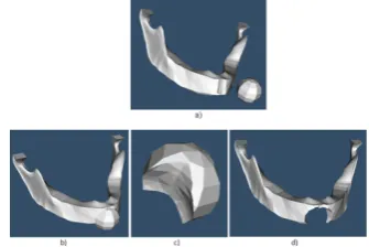
![Fig. 1. Development of methodology concept [1]](https://thumb-us.123doks.com/thumbv2/123dok_us/1661548.119712/22.595.326.515.385.544/fig-development-of-methodology-concept.webp)
