Effective classification of Chinese tea samples in hyperspectral imaging

1

Effective Classification of Chinese Tea Samples

in Hyperspectral Imaging

Timothy Kelman, Jinchang Ren, Stephen Marshall

Centre for excellence in Signal and Image Processing, Dept. of Electronic and Electrical Engineering, University of Strathclyde, Glasgow, G1 1XW, U.K.

{timothy.kelman, jinchang.ren, stephen.marshall}@strath.ac.uk

Abstract— Maximum likelihood and neural classifiers are two typical techniques in image classification. This paper investigates how to adapt these approaches to hyperspectral imaging for the classification of five kinds of Chinese tea

samples, using visible light hyperspectral spectroscopy rather than near-infrared. After removal of unnecessary parts from

each imaged tea sample using a morphological cropper, principal component analysis is employed for feature extraction. The

two classifiers are then respectively applied for pixel-level classification, followed by modal-filter based post-processing for

robustness. Although the samples look similar to the naked eye, promising results are reported and analysed in our

comprehensive experiments. In addition, it is found that the neural classifier outperforms the maximum likelihood classifier

in this context.

Keywords- hyperspectral imaging (HSI), tea classification, principal component analysis (PCA), maximum likelihood classification (MLC), artificial neural network (ANN)

1 INTRODUCTION

Through acquiring information from the contiguous electromagnetic spectrum, hyperspectral imaging enables more accurate and detailed information extraction than either standard colour imaging or the human eye as these can only identify weighted sums of visible light. In general, a hyperspectral image contains spectral information across a large range of spectral bands as well as spatial information about a scene, thus it is referred to as a three dimensional hypercube (two spatial dimensions and one spectral dimension). Due to the abundance of

information in a hypercube, hyperspectral imaging lends itself to many practical applications.

In the past, applications of hyperspectral imaging usually tended to be complex and large, e.g. remote sensing, wide area surveillance and aircraft-based systems [1-2]. With the emergence of desktop based sensors and camera systems in recent years, hyperspectral imaging has significantly advanced. Consequently, it has opened vast opportunities for more challenging applications including those in pharmaceuticals [3], agriculture [4] and food quality testing [5], where lab-based hyperspectral imaging analysis has become feasible.

2 [8-10] and food composition mapping [11], where near-infrared (NIR) hyperspectral spectroscopy is widely employed. This is because NIR, sampled between 700 nm and 2500 nm, allows spectra to be acquired in three modes in terms of reflection, transmission and transflection. More importantly, with the vibration modes in absorbing infrared radiation in different ways, this technique responds to key food components such as C-H, O-H and N-O-H molecular bonds [10]. Although NIR hyperspectral spectroscopy is widely used in food analysis, the imaging system is much more expensive than one using visible light for hyperspectral imaging. In this paper, it is our intention to extend the work done in [12] which tests the effectiveness of food-related analysis using visible hyperspectral spectroscopy to classify five different kinds of Chinese tea samples. The reasons tea samples were chosen for classification are three fold: firstly, this topic has rarely been investigated [13]; secondly, consumption of tea is a world-wide popular activity; and thirdly, tea price varies significantly in terms of brand and associated grades. Since conventional methods for tea analysis and classification need subjective input from domain experts, hyperspectral imaging provides a unique means for objective and consistent quality control even when the samples under examination appear quite similar to each other. Certainly, HSI research has the potential to benefit a huge number of customers through quality analysis and control, such as identifying inferior or even fake products from famous brands.

In hyperspectral imaging, several machine learning and pattern recognition approaches have been proposed for classification. These include artificial neural network (ANN) [16], support vector machine (SVM) [13], minimum distance classifier (MDC) [17] and maximum likelihood classifier (MLC) [17] et al. In principle, all these techniques can be applied in our system. In [12], only MLC was considered. This paper extends this work by also considering ANN. Implementation of these two classifiers and a comparison of their performance are presented in detail in the following sections.

The remaining parts of the paper are organised as follows. Section 2 describes data preparation for pre-processing along with spectrum-based feature extraction and selection. Section 3 discusses how these features are applied for classification, where spatial filtering is introduced as post-processing for improved robustness. Experimental results and quantitative evaluations are presented in Section 4. Finally, concluding remarks are drawn in Section 5.

2 DATA PREPARATION AND FEATURE EXTRACTION

3 2.1 Data Preparation and Pre-processing

In total five different types of tea were used in our experiments: China Black (Tea 1), Lung Ching (Tea 2), Tikuanyin (Tea 3), Yunnan (Tea 4) and Jasmine (Tea 5). All the tea samples were imaged using an Andor Luca EMCCD camera with a Specim V8E spectrograph attached. Samples were placed on a Zolix KSA 11-200S4N motorised stage and illuminated with an Armley 150W Halogen lamp.

For each type of tea, two samples were placed into the compartments of an ice cube tray and imaged

simultaneously to generate a hypercube. Since each tea was imaged twice, 10 hypercubes were produced from the five types of tea. Each hypercube was then scaled using a white and dark reference image so each pixel has a value in the range 0 to 1. For each hypercube, there were 256 spectral bands, however not all of these bands contained information; some were just noise due to camera and the spectrograph not having the same spectral range. This redundant data in each hypercube was removed leaving 170 bands in the range 400 – 800 nm.

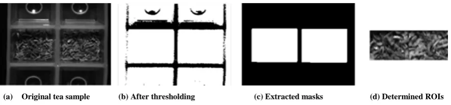
There were a substantial number of non-tea pixels in each of the acquired hypercubes, which were mainly from the container holding the tea samples whilst the data was captured, i.e. the ice cube tray. Therefore, these pixels were excluded so that only valid tea samples remained for classification. To this end, the hypercubes were cropped so that only the tea data was processed.

Rather than using manual image cropping, each hypercube was converted to a binary image and a

morphological opening was performed to leave just two white boxes of tea. The sizes and the locations of these white boxes were then used to crop the hypercube and valid tea samples were extracted as a region of interest in the centre of the cropped cube. The size of each region of interest used was 39 by 51 pixels. This process is shown in Figure 1.

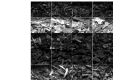
After applying the above cropping process to all 10 hypercubes where each contained two samples from the same tea, 20 different samples were produced. This resulted in 4 samples for each of the 5 teas. Images of these samples at the spectral band of 790 nm are shown in Figure 2. As can be seen at this spectral band, some of the

(a) Original tea sample (b) After thresholding (c) Extracted masks (d) Determined ROIs

4 tea samples appear quite similar to each other, such as Tea 3 (in the third row), Tea 4 (in the fourth row) and also Tea 1 (in the first row). This shows how difficult it is to classify these samples if only one grey level intensity is available, i.e. using a conventional method.

2.2 Feature Extraction and Selection

Since a hypercube contains data derived from a range of contiguous spectral bands, there is a significant volume of highly correlated data, especially in adjacent bands. Processing this high volume of data is computationally expensive and due to the high correlation, potentially inefficient. Therefore, it is essential to extract uncorrelated components as features from this highly correlated data for both efficiency and effectiveness. To achieve this, Principal Component Analysis (PCA) was employed.

PCA is a method used to transform correlated data into a number of uncorrelated variables, known as principal components [14]. The first principal component contains as much of the variance of the data as possible; each subsequent component contains as much of the remaining variance as possible whilst being orthogonal to all previous components. Since most of the information is stored in the first few principal components, the other components can be discarded with very little loss of information. This allows a hypercube to be greatly reduced in size, whilst still retaining most of the information allowing efficient processing. In other words, PCA can be used for both feature extraction and feature selection, and has been widely applied in hyperspectral image analysis [15].

Let X{x1,x2,...,xN} be a hyperspectral image of Nspectral bands. Applying PCA to X will result in a new

listY{y₁,y₂,...,y_M}, where yk|k[1,M] refers to the th

k principal component. Although in theory PCA can generate N principal components, usually only the first 10-20 components are kept thus we haveM N.

5 These remaining components then form a feature vector and are used for classification as discussed in the next section.

3 CLASSIFICATION

Minimum Distance Classifier (MDC) and Maximum Likelihood Classifier (MLC) are both straightforward approaches for classification. In MDC, a sample is assigned to the class with which it has minimum distance to one or all of the samples in that class, which is often used for template matching [18]. Since MDC does not consider the distribution of the samples in the class, it may generate poor results especially when the distribution is biased [17]. MLC, on the other hand, can overcome this drawback as it considers both the mean and

covariance of each class in the training data. This allows the direction as well as the distance from the mean of each class to be taken into account offering an improved performance. In addition, MLC can be easily adapted to work with problems of different numbers of classes and variables making it ideal for this study. Consequently, MLC is selected as one classifier in our system.

Artificial Neural Network (ANN) is also chosen as a classifier that can be directly compared with MLC. ANNs are mathematical models that are based on a biological neural system. They contain weighted connections between neurons that transform an input into an output. The network is trained by looking at pairs of inputs and outputs and adjusting the weights to minimise the error between the network output and a known target. This makes them ideal in a classification problem such as this one.

Implementation details of the two selected classifiers for tea classification are presented below.

3.1 Implementation of MLC and ANN

For the five types of tea, we define them in five classes. The MLC is trained by calculating the mean vector, mi and covariance matrix, C_i for the tea data in each class, ω_i where i[1,5]. Each pixel, x, of the testing set is then classified into the class of the maximum likelihood by

i j >

ω_{i i j} 

 ifg (x) g (x) for all

x ) ( ) ( | -ln = ) (

g_i x C_i|-x-m_i TC_i-1 x-m_i

Regarding the neural classifier, the principle how it works in our system is explained as follows. For a given input vector x(x₁,x₂,...,x_d)T, the output of a single neuron z is determined as

) ( ) ( 1 T



i wixi b

g b g

6 where w(w₁,w₂,...,w_d)Tdenotes a weight vector,g() refers to an activation function to decide whether the perceptron should fire or not. The sigmoid function _{Sig(x)(1e}x₎1 _{is the most popular used activation}

function.

The same process used to compute the output of a single neuron can be used to calculate the output of the whole network in a topological manner. This means that for each neuron, its inputs from other neurons must be computed before determining its output. Consequently, the weight vector and the bias associated to each connection and each node will influence the results, and they can be determined in training or learning process as follows.

Before training the ANN, the topology of the ANN must be specified, and the feed-forward ANN is used. A feed-forward ANN is a multi-layer perceptron (MLPP) which contains three or more layers of neurons, i.e. one input layer, one output layer and at least one hidden layer. With a given training set, a specified activation function and a learning ratio  where (0,1), the learning process for supervised training using the well-known back-propagation algorithm can be described in the following three stages.

First, the initial weights and bias are set randomly between [1,1] to attain a group of outputs z(t) at t1

referring to the first round of iteration. Then, an error function is decided as () ( ) /2

1 2 ) (



 using the

sum of squared error between the estimated output z and the target outputy. Finally, the error signal at the output units is propagated backwards through the whole network to update the weights using the gradient descent rule ij ij w t t w      ()  ()

wherew_ij refers to a weight between the jth node in a given layer and the ith node in the following layer. With

updated weights, we can set tt1 to start a new iteration until the network converges. This can be measured by using a small change ratio of () or a given number of iterations.

3.2 Spatial filtering for post-processing

7 improved the classification accuracy. In addition, each class is assigned a colour so that the results can be visually evaluated. The classification results are presented and analysed in detail in the next section.

4 RESULTS AND DISCUSSIONS

To verify the effectiveness of the proposed method, quantitative evaluation was carried out and is presented in this section. Experiments were performed and the effect of different settings on the classification accuracy is discussed. Basically there were three important parameters in our system, i.e. training percentage, modal filter size and number of principal components used. Details on how these parameters are altered and their effects on the classification accuracy are discussed.

4.1 Test with Different Training Percentages

As shown previously in Figure 2, we had 5 tea classes, and each contained four blocks of pixel based samples. If we take 1-3 block(s) of pixels for training and use the remaining for testing, the training percentage will be either 25%, 50% or 75%. For a given training percentage, say 25%, one block of the pixels from each class was used for training and the others for testing, thus four groups of training/testing results were produced for cross validation. The average accuracy was then obtained as a measurement of the overall performance.

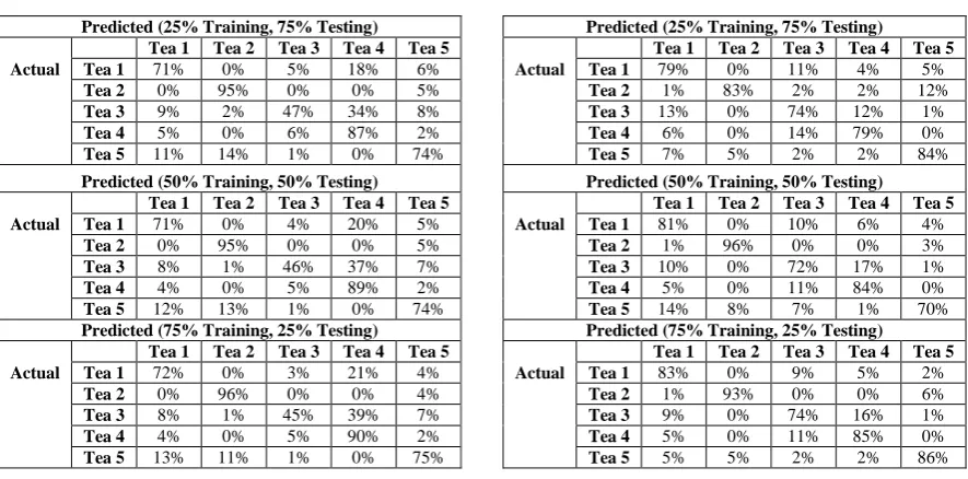
Table 1: MLC cross validated confusion matrices Table 2: ANN cross validated confusion matrices

Predicted (25% Training, 75% Testing) Tea 1 Tea 2 Tea 3 Tea 4 Tea 5 Actual Tea 1 71% 0% 5% 18% 6%

Tea 2 0% 95% 0% 0% 5%

Tea 3 9% 2% 47% 34% 8%

Tea 4 5% 0% 6% 87% 2%

Tea 5 11% 14% 1% 0% 74%

Predicted (50% Training, 50% Testing) Tea 1 Tea 2 Tea 3 Tea 4 Tea 5 Actual Tea 1 71% 0% 4% 20% 5%

Tea 2 0% 95% 0% 0% 5%

Tea 3 8% 1% 46% 37% 7%

Tea 4 4% 0% 5% 89% 2%

Tea 5 12% 13% 1% 0% 74%

Predicted (75% Training, 25% Testing) Tea 1 Tea 2 Tea 3 Tea 4 Tea 5 Actual Tea 1 72% 0% 3% 21% 4%

Tea 2 0% 96% 0% 0% 4%

Tea 3 8% 1% 45% 39% 7%

Tea 4 4% 0% 5% 90% 2%

Tea 5 13% 11% 1% 0% 75%

Predicted (25% Training, 75% Testing) Tea 1 Tea 2 Tea 3 Tea 4 Tea 5 Actual Tea 1 79% 0% 11% 4% 5%

Tea 2 1% 83% 2% 2% 12%

Tea 3 13% 0% 74% 12% 1%

Tea 4 6% 0% 14% 79% 0%

Tea 5 7% 5% 2% 2% 84%

Predicted (50% Training, 50% Testing) Tea 1 Tea 2 Tea 3 Tea 4 Tea 5 Actual Tea 1 81% 0% 10% 6% 4%

Tea 2 1% 96% 0% 0% 3%

Tea 3 10% 0% 72% 17% 1%

Tea 4 5% 0% 11% 84% 0%

Tea 5 14% 8% 7% 1% 70%

Predicted (75% Training, 25% Testing) Tea 1 Tea 2 Tea 3 Tea 4 Tea 5 Actual Tea 1 83% 0% 9% 5% 2%

Tea 2 1% 93% 0% 0% 6%

Tea 3 9% 0% 74% 16% 1%

Tea 4 5% 0% 11% 85% 0%

Tea 5 5% 5% 2% 2% 86%

Under different training percentages, Table 1 and Table 2 show the cross validation results for the five types of tea for MLC and ANN respectively. Looking at just the MLC performance, firstly, we can see that the

8 around 46%, and this shows that Tea 3 was the least identifiable. Thirdly, it is interesting to see that the

classification accuracy did not improve with the increasing training percentage. This means that more training samples made no additional contribution to the estimate of the class mean vector and covariance matrix . One reason might be that at a training percentage of 25% and had already been accurately estimated, especially since PCA was used.

The performance of ANN, on the other hand, was noticeably better. The classification accuracy was high for all teas at all percentages, i.e. no less than 72%. The accuracy of Tea 2 and Tea 4 was actually slightly lower than when using MLC but the accuracy of Tea 3 as significantly higher. Unlike the MLC method, the overall classification accuracy did increase with the training percentage. This improvement however, was only slight and was outweighed by the extra computational costs of using more training data.

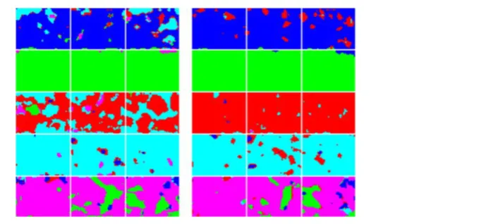
Since each pixel was assigned a colour during classification, a visual representation of the classification results was also produced. One of the testing results for MLC and ANN (at training percentage of 25%) is shown in Figure 3. From Figure 3, we can clearly see how these teas were misclassified with MLC. Although a few pixels in Tea 3 were wrongly classified as Tea 4, more pixels were classified as Tea 3 than as any other. Therefore, it was possible to classify the whole cube as Tea 3 and allow correct classification using MLC. Such a strategy could also have been applied to each of the cubes in such a context. With the ANN result, however, the high classification percentage made it easy for each tea to be classified with only a small number of pixels being wrongly classified in each case.

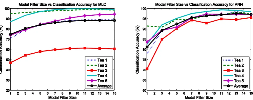
9 4.2 Test with Different Sizes of Modal Filter

Different sizes of modal filter were tested to evaluate their performance as post-processing. The training percentage was varied as in the previous section and the results were averaged to produce the plots shown in Figure 4. The filter size was increased from 1 (no filter) to 15 × 15 pixels. In the case of MLC, it can be seen that increasing the filter size improved classification performance up to a size of around 11 × 11 pixels. Increasing the filter size beyond this had little effect on the performance. In addition, a modal filter of the size more than 11 × 11 pixels may degrade the performance for Tea 2, Tea 3 and Tea 4; although for Tea 5 the performance was significantly improved when the filter size increases. This demonstrates that the

post-processing may have conflicting effects on different teas. As a result, we may need to apply a specially designed structuring element, perhaps similar to the shape of a tea leaf, rather than the square one used in this test. In the case of ANN, the modal filtering had a significant effect. Increasing the filter size up to 13 × 13 pixels improved classification accuracy, but after 7 × 7 pixels, this improvement was very slight and is outweighed by the extra computational cost of using a larger structuring element. Increasing the filter size beyond 11 × 11 pixels had a negative impact on Tea 4 and beyond 13 ×13 pixels it started to negatively affect Tea 1 and Tea 2 also.

Modal filtering provides a method of increasing the accuracy of both classifiers, but in particular , ANN performance sees notable improvement for all classes.

Figure 4: Classification accuracy under different modal filter sizes from MLC (left) and ANN (right) classifiers.

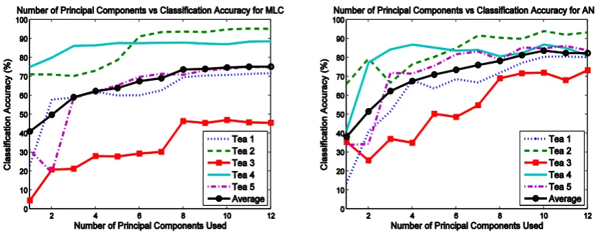
4.3 Test with Different Numbers of Principal Components

A similar test was also applied to various numbers of principal components. The number of principal

10 previous section. The classification accuracy for this test is shown in Figure 5 for both MLC and ANN.

In general, increasing the number of components helped to improve the classification accuracy. For Tea 2 and Tea 4, the accuracy was over 70% even with only the first two components in both MLC and ANN cases. This again shows that these two teas were relatively more distinguishable. For Tea 5, MLC required the first 8 components to achieve an accuracy of around 70% where ANN only required the first 3. Tea 3 required the first 8 components for MLC classification to achieve an accuracy of nearly 50 % but only the first 5 components were needed for ANN. This shows that performance of MLC and ANN is similar at lower component numbers, but ANN starts to outperform MLC as the component number increases. This on one hand indicates the difference among these tea samples and classification methods. On the other hand, it might be useful to apply subsequent feature selection dependent on the classification algorithm leading to more robust classification.

Figure 5: Classification accuracy under different numbers of principal components from MLC (left) and ANN (right) classifiers.

4.4 Optimising the ANN Classifier

11 4.5 Cohen’s Kappa

So far, only the classification percentage has been used as a measure of performance. This measure does not compensate for the fact that some pixels could be correctly classified due to random chance. Cohen’s Kappa, κ, takes into account the probability of chance agreement and is calculated as follows:

( ) ( ) ( )

where ( ) is observed agreement and ( ) is the probability of random agreement. Table 3 summarises Cohen’s Kappa for the classified results before and after modal filtering, respectively.

Table 3: Cohen's Kappa under different training ratios with or without modal filtering

Training

Percentage Classifiers

Cohen's Kappa

No modal filter With 5x5 modal filter

25 MLC 0.69 0.80 ANN 0.77 0.92 50 MLC 0.69 0.80 ANN 0.72 0.89 75 MLC 0.69 0.80 ANN 0.80 0.95

It is interesting to note that Cohen’s Kappa coefficient is insensitive to different training percentages for MLC, both with and without filtering whereas the coefficient increases with training percentage for ANN. This can be explained by the fact that MLC classification accuracy is not improved by increasing classification percentage and so it follows that Cohen’s Kappa would also not see an improvement.

As expected, Cohen’s Kappa increases with the introduced modal filtering. With 5 x 5 modal filtering, all the Cohen’s Kappa coefficients are high, showing that there is good classification agreement.

5 CONCLUSION

12 produce negative effect. Finally, MLC required 8 principal components to achieve a satisfactory classification rate for all teas, whereas ANN only required the first 5. In both cases more than 10 principal components offered no improvement to the accuracy of classification.

6 REFERENCES

[1] A. F. H. Goetz, G. Vane, J. E. Solomon, and B. N. Rock, “Imaging Spectrometry for Earth Remote Sensing,” Science, 228(4704), 1147-1153, 1985

[2] H. Ren; C. Chang, “Automatic spectral target recognition in hyperspectral imagery,” IEE Trans. Aerospace and Electronic Systems, 39(4), 1232- 1249, 2003

[3] Y. Roggo, A. Edmond, P. Chalus, M. Ulmschneider, “Infrared hyperspectral imaging for qualitative analysis of pharmaceutical solid forms,” Analytica Chimica Acta, 535(1-2), 79-87, 2005

[4] Y. Uno, S. O. Prasher, R. Lacroix, P. K. Goel, Y. Karimi, A. Viau, R. M. Patel, “Artificial neural networks to predict corn yield from Compact Airborne Spectrographic Imager data,” Computers and Electronics in Agriculture, 47(2), 179-161, 2005

[5] Q. Wu, D. Zhu, C. Wang, Z. Ma, J. Wang, “Recognition of wheat preharvest sprouting based on hyperspectral imaging,” Optical Engineering, 51(11), 2012

[6] G. K. Naganathan, L. M. Grimes, J. Subbiah, C. R. Calkins, A. Samal, G. E. Meyer, “Visible/near-infrared hyperspectral imaging for beef tenderness prediction,” Computers and Electronics in Agriculture, 64(2), 225-233, 2008

[7] D. P. Ariana, R. F. Lu, and D. E. Guyer, “Near-infrared hyperspectral reflectance imaging for detection of bruises on pickling cucumbers,” Computers and Electronics in Agriculture, 53, 60-70 2006

[8] H. K. Noh and R. F. Lu, “Hyperspectral laser-induced fluorescence imaging for assessing apple fruit quality,” Postharvest Biol. Technol., 43, 193-201, 2007

[9] B. Park, W. R. Windham, K. C. Lawrence, and D. P. Smith, “Contaminant classification of poultry hyperspectral imagery using a spectral angle mapper algorithm,” Biosyst. Eng., 96, 323-333, 2007

[10] J. Qiao, N. Wang, M. O. Ngadi, A. Gunenc, M. Monroy, C. Gariépy, and S. O. Prasher, “Prediction of drip-loss, pH, and color for pork using a hyperspectral imaging technique,” Meat science, 76, 1-8, 2007

[11] A. Chau, M. Whitworth, C. Leadley, and S. Millar, “Innovative sensors to rapidly and non-destructively determine fish freshness,”

Seafish, 2009

[12] S.J. Millar, M.B. Whitworth, A. Chau, and J. R. Gilchrist, “Mapping food composition using NIR hyperspectral imaging,” New Food, 3, 2008

[13] T. Kelman, J. Ren, and S. Marshall, “Classification of Chinese Teas samples for Food Quality Control using Hyperspectral Imaging,”

Proceedings of Hyperspectral Imaging Conference, 2011

[14] J. Zhao, Q. Chen, J. Cai, and Q. Ouyang, “Automated tea quality classification by hyperspectral imaging,” Applied Optics, 48(19), 3557-35564, 2009

13

[16] G. Shaw, D. Manolakis, “Signal processing for hyperspectral image exploitation,” Signal Processing Magazine, IEEE , 19(1), 12-16, 2002

[17] P. K. Goel, S. O. Prasher, R. M. Patel, J. A. Landry, R. B. Bonnell, and A. A. Viau, “Classification of hyperspectral data by decision trees and artificial neural networks to identify weed stress and nitrogen status of corn,” Computers and Electronics in Agriculture, 39(2),67-93, 2003

[18] J. Richards, X. Jia, Remote Sensing Digital Analysis: An Introduction, 4th _{Edition, Chapter 8, Springer-Verlag, 2006}