A&A 541, A90 (2012)
DOI:10.1051/0004-6361/201118720 c
ESO 2012
Astronomy
&
Astrophysics
Atomic data for astrophysics: Fe
x
soft X-ray lines
G. Del Zanna
1, P. J. Storey
2, N. R. Badnell
3, and H. E. Mason
11 DAMTP, Centre for Mathematical Sciences, Wilberforce Road, Cambridge, CB3 0WA, UK e-mail:[email protected]
2 Department of Physics and Astronomy, University College London, Gower Street, London, WC1E 6BT, UK 3 Department of Physics, University of Strathclyde, Glasgow, G4 0NG, UK
Received 22 December 2011/Accepted 14 February 2012
ABSTRACT
New atomic calculations for Fexare presented. They focus on the need to model the soft X-ray spectrum and in particular the line at 94.0 Å which is the dominant contribution to the Solar Dynamics Observatory (SDO) Atmospheric Imaging Assembly (AIA) 94 Å band in quiet Sun conditions. This line, and others in the band, are due to strong decays fromn=4 levels. We present new large-scale R-matrix (up ton=4) and distorted-wave (DW, up ton=6) scattering calculations for electron collisional excitation and compare them to earlier work. We find significant discrepancies with previous calculations. We show that resonances significantly increase the cross-sections for excitations from the ground state to somen=4 levels, in particular to those in the 3s2 3p4 4s configuration. Cascading from higher levels is also important. We suggest a new identification for the 3s 3p6 2S
1/2–3s 3p54s2P3/2transition, that has a predicted intensity larger than the decays from the 3s23p44s levels which were identified by Edlén in 1936. The results presented here are relevant to our understanding of transitions fromn=4 levels in a wide range of other ions.
Key words.atomic data – line: identification – Sun: corona – techniques: spectroscopic
1. Introduction
The soft X-ray (50–170 Å) spectrum of the quiet and active Sun is rich inn = 4 → n = 3 transitions from highly ionised iron ions, from Feviito Fexvi(see, e.g.Fawcett et al. 1968). Very little atomic data are currently available for these ions and the majority of the spectral lines still await firm identification. Soft X-ray spectra of stellar coronae are routinely observed with the Chandra Low Energy Transmission Grating spectrometer (LETG, seeBrinkman et al. 2000).
The Solar Dynamic Observatory (SDO) Extreme ultravi-olet Variability Experiment (EVE) (Woods et al. 2010) has also been providing soft X-ray spectra. The SDO Atmospheric Imaging Assembly (AIA, see Lemen et al. 2011) has been observing (for the first time routinely) the solar corona in two broad-bands (among others) centred in the soft X-rays, around 94 and 131 Å. These SDO/AIA observations provide unprecedented coverage in terms of spatial and temporal reso-lutions, and can provide new diagnostic applications, once the atomic data are well understood. As shown inO’Dwyer et al. (2010) andDel Zanna et al.(2011), these bands are dominated by Fex and Feviii in normal quiet Sun conditions. However, several unidentified spectral lines have been observed in the AIA passbands with high-resolution grazing incidence solar spectrometers (cf.Behring et al. 1976;Manson 1972).
The atomic data for Feviii and Feix relevant for the soft X-rays have recently been discussed inO’Dwyer et al.(2012),
The full dataset (energies, transition probabilities and rates)
are available in electronic form at our APAP website (www. apap-network.org) as well as at the CDS via anonymous ftp to
cdsarc.u-strasbg.fr(130.79.128.5) or via
http://cdsarc.u-strasbg.fr/viz-bin/qcat?J/A+A/541/A90
where new distorted wave (DW) scattering calculations for these two ions were presented.
This paper focuses on the atomic data for the Fex n = 4 → n = 3 transitions. One of the main transitions is centred at 94 Å and is expected to provide the dominant signal to the SDO/AIA 94 Å band in quiet Sun conditions. Large discrep-ancies (a factor of six) between predicted and observed count rates in this band have been reported (cf.Aschwanden & Boerner 2011), which could in part be ascribed to problems in the atomic data for Fex. Indeed, as shown byMalinovsky et al.(1980), large (at least a factor of two) discrepancies between predicted and ob-served intensities have been found to be present for all the 3s23p4 4s decays to the ground state.
We set out to resolve these discrepancies with a new set of calculations. We encountered along the way a series of problems and issues with the atomic physics model which turn out to be quite general and very interesting.
These Fex transitions are of particular significance for the history of the solar corona. In fact, the famous first identification of a coronal line was given byEdlén(1942) (upon suggestion from Grotrian 1939) as the Fex forbidden2P
3/2–2P1/2
transi-tion within the ground configuratransi-tion. Grotrian’s suggestransi-tion was based on the pioneering laboratory work by Edlén in the 1930’s on the identifications of the soft X-ray lines, in particular the Fex3s23p44s decays to the ground (Edlén 1937).
The paper is organised as follows. In Sect. 2, we give a brief review of previous soft X-ray observations and atomic cal-culations. In Sect. 3 we outline the methods we adopted for the scattering calculations. In Sect. 4 we present our results and in Sect. 5 we reach our conclusions with respect to Fex and other ions.
2. Previous observations and atomic data for Fex
A detailed discussion of the identifications, the historical con-text, and the atomic data for then =2,3 configurations, giving rise to spectral lines from the EUV to the visible was presented in Del Zanna et al.(2004) and is not repeated here.Del Zanna et al. (2004) presented new identifications and a set of new observed energies that are adopted here. The energies of the 3s23p43d
lev-els have all been confirmed with recent, accurate EUV observa-tions with the Hinode EUV Imaging Spectrometer (Del Zanna 2012).
For the soft X-rays (n=4 →n =3 transitions), Edlén car-ried out the first work on the identification of some 3s23p44s
de-cays to the ground. This was followed by the monumental work byFawcett et al.(1972), where a number of lines arising from the 3s23p44l(l=s, p, d, f) levels were identified. It is important
to keep in mind that only lines with strong oscillator strengths were identified, that some identifications were tentative, and that a large number of lines in the laboratory spectra were left uniden-tified. Not all of Fawcett’s work has been adopted within the NIST compilation.
We have re-analysed some of Fawcett’s plates as part of a larger project to sort out the identifications in the Fe soft X-ray spectrum. We have also considered various other ex-perimental sources, in particular the excellent (still the best) grazing-incidence spectra of the full Sun taken in the late 1960s during rocket flights (see Manson 1972; Behring et al. 1972; Malinovsky & Heroux 1973). Virtually all spectral lines, even at high resolution, are blended. The majority of lines are still unidentified and very few reliable atomic data are available. For these reasons, a full comparison and benchmarking with observations is deferred to a future paper.
The first comprehensive collision strength calculation for Fex was published by Mason (1975). She used the University College London (UCL) distorted-wave DW code (Eissner 1998), which includes the superstructure program (Eissner et al. 1974). Only the lowest 3s2 3p5, 3s 3p6, and
3s23p43d configurations were included.
Malinovsky et al.(1980) also used the UCL-DW code to cal-culate collision strengths, but this time for the n = 4 levels. The authors focused on the 3s23p4 4s decays to the ground.
Large (factors of 5 to 6) discrepancies between the observed (by Malinovsky & Heroux 1973) and calculated line intensi-ties were found. Cascading from higher levels was found to be important, but difficult to estimate. The inclusion of cascading contributions improved the comparison, but still left discrepan-cies of a factor of two or more. To our knowledge, no other calculations for then=4 levels have been published since.
For then=3 levels there are a number of calculations.Pelan & Berrington(2001) published, as part of the Iron Project, a full Breit-Pauli R-matrix calculation for a target including 180 lev-els arising from the five lowestn =3 configurations. Collision strengths were calculated for a total of 7460 energy points in the resonance region (up to 9.95 Ryd).Pelan & Berrington(2001) only published excitation data from the three levels arising from 3s2 3p5, 3s 3p6. Given that there are a number of metastable
states for this ion, collision data from those states are also needed (Del Zanna et al. 2004). Hence, a new calculation was needed. In addition, the “top-up” procedure was not applied inPelan & Berrington(2001), and collision strengths for the strongest lines were found to be inaccurate (seeAggarwal & Keenan 2005).
Del Zanna et al. (2004) repeated the earlier Pelan & Berrington(2001) calculation for the lowest 31 levels due to the 3s23p5, 3s 3p6, and 3s23p4 3d configurations but with the
addition of high partial wave top-up. These latter data have been used since 2005 within the CHIANTI database (Dere et al. 1997; Landi et al. 2006). Good overall agreement between predicted and observed line intensities using these atomic data was found inDel Zanna et al.(2004) and later inDel Zanna(2012).
Aggarwal & Keenan(2005) later performed a Dirac Atomic R-matrix Code (DARC) calculation for the lowest 90 levels of the 3s23p5, 3s 3p6, and 3s23p43d, 3s 3p53d, 3s23p33d2 con-figurations. This calculation was in some respects quite similar toPelan & Berrington(2001). However, large differences (up to a factor of two) were found for some allowed transitions such as the 1–3. Relatively good agreement between theAggarwal & Keenan(2005) andDel Zanna et al. (2004) is found however, as shown below.
3. Methods
The atomic structure calculations were carried out using the
autostructureprogram (Badnell 1997) which constructs target wavefunctions using radial wavefunctions calculated in a scaled Thomas-Fermi-Dirac statistical model potential with a set of scaling parameters.
The Breit-Pauli distorted wave calculations were carried out using the recent development of theautostructure code, described in detail in Badnell (2011). The continuum torted waves are calculated using the same form for the dis-torting potential as specified for the target, but now for the (N+1)-electron problem. The electrostatic (N+1)-electron in-teraction Hamiltonian for the collision problem is determined in an unmixed LS-coupling representation. It is then transformed to an LSJ representation. The full (N+1)-electron interaction Hamiltonian is transformed to a full Breit-Pauli jK-coupling rep-resentation (i.e. including both configuration and fine-structure target mixing) in the same manner as is done for the (inner-region) Breit-Pauli R-matrix method. Collision strengths are cal-culated at the same set of final scattered energies for all tran-sitions. “Top-up” for the contribution of high partial waves is done using the same Breit-Pauli methods and subroutines im-plemented in the R-matrix outer-region code STGF. The pro-gram also provides radiative rates and infinite energy Born limits. These limits are particularly important for two aspects. First, they allow a consistency check of the collision strengths in the scaledBurgess & Tully(1992) domain (see alsoBurgess et al. 1997). Second, they are used in the interpolation of the collision strengths at high energies when calculating the Maxwellian averages.
The R-matrix method used in the scattering calculation is described inHummer et al.(1993) andBerrington et al.(1995). We performed the calculation in the inner region inLS coupling and included mass and Darwin relativistic energy corrections.
The outer region calculation used the intermediate-coupling frame transformation method (ICFT) described byGriffin et al. (1998), in which the transformation of the multi-channel quan-tum defect theory unphysical K-matrix to intermediate cou-pling uses the so-called term-coucou-pling coefficients (TCCs) in conjunction with level energies.
Dipole-allowed transitions were topped-up to infinite partial wave using an intermediate coupling version of the Coulomb-Bethe method as described byBurgess(1974) while non-dipole allowed transitions were topped-up assuming that the collision strengths form a geometric progression in J (see Badnell & Griffin 2001).
G. Del Zanna et al.: Atomic data for astrophysics: Fexsoft X-ray lines
Table 1.List of a few among the strongest Fexlines in the soft X-rays.
i–j Levels Int Int Int Int Int Aji(s−1) λexp(Å) λth(Å)
DW (n=4) DW (n=6) RM RM+ CHIANTI DW (n=6)
1–202 3s23p5 2P
3/2–3s23p44s2D5/2 5.3×10⁻³ 7.5×10⁻³ 9.2×10⁻³ 1.2×10⁻² 8.9×10⁻³ 3.7×10¹⁰ 94.012 90.46 3–429 3s 3p6 2S
1/2–3s 3p54s2P3/2 1.7×10⁻² 1.4×10⁻² 1.8×10⁻² 1.8×10⁻² 5.9×10⁻³ 4.8×10¹⁰ - 91.48 22–267 3s23p43d2G
9/2–3s23p44p2F7/2 2.5×10⁻³ 2.8×10⁻³ 3.2×10⁻³ 3.4×10⁻³ 2.8×10⁻³ 1.4×10¹⁰ 139.869 135.95 1–370 3s23p5 2P
3/2–3s23p44d2D5/2 1.1×10⁻³ 1.9×10⁻³ 1.4×10⁻³ 1.6×10⁻³ 6.2×10⁻³ 7.2×10¹⁰ 77.865 75.17 21–488 3s23p43d2F
5/2–3s23p44f2G7/2 2.0×10⁻³ 1.9×10⁻³ 2.2×10⁻³ 2.2×10⁻³ - 1.6×10¹¹ 103.319 100.39 1–30 3s23p5 2P
3/2– 3s23p43d2D5/2 1.0 1.0 1.0 1.0 1.0 1.9×10¹¹ 174.531 163.29 Notes.The relative intensities (photons)Int=NjAji/Neare normalised to the strongest EUV transition (1–30) and were calculated at a coronal
electron density of 108 cm−3 and log T[K]=6.05. The DW intensities were obtained with the DW calculations. The RM are obtained from the R-matrix calculations, i.e. only includingn= 3,4 levels. The RM+DW is from a combined model where the RM model is augmented by including excitation and radiative data forn=5,6 levels from the DW calculation. The last column shows the values calculated with the current CHIANTI model.A-values (s−1) as obtained from the RM model are shown, as well as experimental (λ
exp) and theoretical (λth, from the RM model) wavelengths.
Burgess & Tully(1992) scaled domain. The high-energy limits were calculated withautostructurefor both optically-allowed (seeBurgess et al. 1997) and non-dipole allowed transitions (see Chidichimo et al. 2003). All the transitions from the ground configuration were visually inspected. General agreement in the background collision strengths was found with the DW values, and at high energies with the limit points.
The temperature-dependent effective collisions strength
Υ(i− j) were calculated by assuming a Maxwellian electron distribution and linear integration with the final energy of the colliding electron.
4. Results
Several calculations have been performed with different size tar-get expansions and corresponding ion population models have been constructed to predict line intensities and compare with observations. A summary of our investigations is presented here.
4.1. Initial DW calculations
We started with various DW calculations systematically increas-ing the number of configurations up to and includincreas-ing those with n = 6 valence orbitals. As shown byDel Zanna et al.(2004), a number of metastable levels within the 3s23p4 3d
configura-tion become significantly populated at coronal densities (up to level 24). Hence, DW excitation rates from the lowest 24 levels have been calculated.
We then performed separate structure calculations for each ion model to calculate all of the radiative data for all transitions among the levels. This ensures that all the cascading from the tar-get configurations is included. We then calculated the level pop-ulations and the relative line intensities so as to find out which lines are expected to be strongest in quiet Sun conditions.
Following Malinovsky et al. (1980), the intensities of the soft X-ray lines (4s–3p) have been considered relative to the strongest EUV line (3d–3p). Table 1 shows the details for a few transitions among the strongest lines from the mainn = 4 configurations. The relative intensities obtained from two purely DW runs, which are described below, are displayed in the first two intensity columns of Table 1. The first DW ion model includes almost all possible of the n = 3,4 config-urations. The second DW ion model also includes the main n=5,6 configurations. The other ion models we built produce
similar results. The following two columns show the results ob-tained with the models described below, while the last one shows the values calculated with the current CHIANTI model, which has theMalinovsky et al.(1980) collisional data.
One of the strongest lines in the soft X-rays is the 3s2 3p5 2P
3/2–3s2 3p4 4s 2D5/2 identified by Edlén (1937)
at 94.012 Å. The relative intensity with then = 4 DW model is 5.3×10⁻³(in photons), i.e. almost six times weaker than
ob-served (3.2×10⁻²) byMalinovsky & Heroux(1973) and about a factor of two lower than calculated byMalinovsky et al.(1980) (1.0×10⁻²). As shown byMalinovsky et al.(1980), cascading
from higher levels does increase the population of the 4s2D 5/2,
but only at the 10−20% level. Our largen =6 DW model pre-dicts a relative intensity of 7.5×10⁻³, larger as expected, but also lower than the value calculated byMalinovsky et al.(1980) (1.2×10⁻²).
Similar discrepancies betweenMalinovsky et al.(1980) and our results are present for the other lines in the same transi-tion array. The differences between our results andMalinovsky et al.(1980) in the calculated values should not be present since very similar (DW) scattering approximations have been used. Actually, for dipole-allowed lines,Malinovsky et al.(1980) only calculated DW collision strengths at 12 and 20 Ryd, while a semi-classical approximation, based on Burgess (1964), was used at 40 and 80 Ryd. It is not entirely clear which set of con-figurations was used byMalinovsky et al.(1980). However, we have run a DW calculation including the same set of configura-tions as listed in their paper, and the differences remain. It turns out that the differences are due to significantly overestimated collision strengths byMalinovsky et al.(1980), as shown below. The overestimation of collision strengths by Malinovsky et al. (1980) only makes the problem worse in terms of comparison with solar data. The cause could in part be due to an incorrect photometric calibration of the Malinovsky & Heroux (1973) spectrum in the soft X-rays. A discussion of this is deferred to a future paper. However, even just consid-ering the soft X-rays, significant problems are still present. In particular, the DW calculations clearly indicate that the 3s 3p6 2S
1/2−3s 3p5 4s 2P3/2 transition is almost three times
stronger than the 3s2 3p5 2P
3/2−3s2 3p4 4s 2D5/2 94 Å line.
This is caused by a strong forbidden excitation from the ground state to the 3s 3p5 4s 2P
3/2, with collision strengths much
The 3s 3p5 4s 2P3/2 level then decays via a strong
dipole-allowed transition. This transition has not been identified pre-viously. However, our ab-initio calculations predict this line to fall around 95−96 Å. At around these wavelengths there are no lines in the solar spectrum which are two or three times stronger than the 94 Å line. The same holds for the laboratory plates from Fawcett which we have analysed.
All of the DW calculations we have carried out produced similar values. We have also run similar calculations for other iron ions and found the same situation: strong transitions from 3s 3pq4s, not identified by Edlén or Fawcett. In general, we have found significant numbers of unidentified lines, stronger than those that have been identified, which complicates the bench-marking of the atomic data. As stated previously, a full dis-cussion of benchmarking with solar and laboratory spectra is beyond the scope of this paper and is deferred to a future paper. The only reasonable solution to the problem is that all of the excitations to the 3s23p44s levels are significantly
underes-timated by the DW calculations. Indeed, we previously found a similar situation for Feix, as discussed inO’Dwyer et al.(2012). We found that there are resonances which increase significantly the collision strengths to the 3s2 3p5 4s levels. A purely (non-resonant) DW calculation would underestimate by at least a fac-tor of two the intensities of any decays from these levels, com-pared to what is obtained with an R-matrix calculation (Storey et al. 2002).
4.2. Estimate of resonance contribution
A full R-matrix calculation withn =4,5 levels is challenging, so before embarking on such a calculation we performed vari-ous DW calculations to estimate which configurations would be likely to be producing resonances in the collision strengths for the spectroscopically important configurations/levels. For each model, we calculated all the collision strengths at threshold be-tween all the levels. The details of two of such calculations are given below. Here, we are using results form the larger of the two calculations.
To assess which configurations would contribute signifi-cantly, we considered two steps, the first being dielectronic cap-ture which is directly proportional to the excitation collision strengths. Only levels with similar excitations from the ground configuration can be important. The second step is the Auger de-cay, which has a rate proportional to the excitation cross-section between the levels (Burgess 1965). If we identify all first step excitations that are stronger or comparable with the direct ex-citations of interest then we necessarily have all possible can-didates for strong resonance contributions. Whether these do in fact contribute strongly, depends on step two.
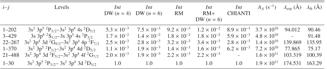
Consider as an example the 3s2 3p44s2D
5/2 level which is
populated by a dipole excitation from the ground state but with the relatively small threshold collision strength of 0.027 (see Fig.1). The collision strength for the dipole forbidden excitation of the 3s23p44p2P
3/2from the ground state, on the other hand
is large, 0.6 at threshold, implying a large dielectronic capture rate to the resonances converging on this state. These resonances can autoionize into all possible open channels but the DW cal-culations show that the two main routes leave the ion either in its ground state or in the 3s23p4 4s2D
5/2 level. The threshold
collision strengths, 0.6 and 2.1 respectively, provide an estimate of the branching ratio between these routes, with 80% leaving the ion in the 3s2 3p4 4s 2D
5/2 level. Since the average effect
of the resonances converging on the 3s2 3p4 4p 2P
[image:4.595.310.558.77.254.2]3/2 can be
Fig. 1.The main levels related to the 3s23p44s2D
5/2, which produces the 94.012 Å line. The values of the collision strengths at threshold among the levels and from the ground state are shown.
thought of as an extrapolation of the threshold collision strength to negative final energy, this implies that the collision strength for excitation to the 3s2 3p4 4s 2D
5/2 level will be enhanced
by 0.48 in the energy interval between the 3s23p44s2D5/2and
3s23p44p2P
3/2levels, almost 20 times the value for direct
exci-tation. We will show below that the result of a detailed R-matrix treatment of the resonances gives a similar increase. These are estimates based on total threshold collision strengths. A full treatment involves detailed consideration of all the scattering channels (see, e.g.Petrini 1970).
Other contributions could also come from other configura-tions connected to the 3s23p4 4s by a dipole coupling, such as
3s23p33d 4s, 3s 3p5 4s and 3s23p4 np,n ≥5. The latter
con-figurations are especially interesting given the large contribution fromn =4. In practice we do not find large collision strengths for excitation of the 3s23p4np forn=5,6 from the ground and
also there are additional Auger channels reducing the branching ratio to the 3s23p44s levels.
We used the same approach to assess the importance of reso-nance contributions to the other levels of then=4,5 configura-tions. We found that the 3s 3p54s levels are not expected to have
significant contributions from resonances. The 3s2 3p4 4p lev-els have significant resonance contributions, mainly from the 3s23p44d, 3s23p44f and 3s23p33d2. The 3s23p44d levels are expected to have some contributions, mainly from the 3s23p44f.
On the other hand, the 3s23p44f levels are not expected to have
significant resonance contributions from othern = 4,5 levels. A similar picture applies to then=5 levels.
In summary, with the exception of a small contribution from the 3s2 3p4 5p levels to the 3s2 3p4 4s (and 3s2 3p4 4p), the
main resonance contribution to then=4 spectroscopic configu-rations comes from configuconfigu-rations within then=4 complex. We have therefore chosen to proceed with a full R-matrix calculation including all the mainn=3,4 configurations.
4.3. The R-matrix and DW calculations for then=3,4 levels
G. Del Zanna et al.: Atomic data for astrophysics: Fexsoft X-ray lines
[image:5.595.72.259.369.572.2]Fig. 2.The term energies of the target levels (32 configurations) for then=4 calculations. The 218 terms which produce levels having energies below the dashed line have been retained for the close-coupling expansion.
Table 2.The target electron configuration basis and orbital scaling parametersλnlfor the R-matrix and DW runs for then=3,4 levels.
Configurations
Even Odd λnl
3s 3p6 3s23p5 1s 1.41548 3s23p43d 3s 3p53d 2s 1.12358 3s23p44s 3s23p33d2 2p 1.06501 3s 3p43d2 3s23p44p 3s 1.12476 3p63d 3s 3p54s 3p 1.09729 3s23p44d 3s23p44f 3d 1.11252 3s 3p54p 3s23p33d 4s 4s 1.21772
3s23p33d 4p 3p53d2 4d 1.20247 3p64s 3s 3p54d 4p 1.19803 3s 3p54f 3s23p33d 4d 4f 1.35751 3s 3p43d 4s 3p64p
3s23p33d 4f 3s 3p43d 4p 3p64d 3p64f 3s 3p43d 4d 3s 3p43d 4f 3p53d 4p 3p53d 4s 3p53d 4f 3p53d 4d
Notes. The configurations below the line have been included in the CI expansion.
levels arising from the lowest 218LS terms were retained for the scattering calculation. We have performed both an ICFT R-matrix and a DW calculation using the same basis. They are both large-scale calculations.
Table 3 presents a selection of fine-structure target level energies Et, compared to experimental energies Eexp (from
Del Zanna et al. 2004, for the n = 3 levels; otherwise from Fawcett et al. 1972). There is good overall agreement in terms of energy differences between levels. A set of “best” energiesEb
was obtained with a quadratic fit between theEexpandEtvalues.
TheEbvalues were used (together with theEexpones) within the
R-matrix calculation to obtain an accurate position of the reso-nance thresholds. The resoreso-nances in the transitions to then =4 levels are close to thresholds, therefore it is important to position
them as accurately as possible. TheEexpandEbvalues were also
used when calculating radiative rates.
The expansion of each scattered electron partial wave was done over a basis of 25 functions within the R-matrix bound-ary and the partial wave expansion extended to a maximum total orbital angular momentum quantum number of L = 16. This produced accurate collision strengths up to about 80 Ryd. The resulting effective collision strengths are accurate up to an elec-tron temperature of about 107K. However, the interpolation for all allowed transitions utilizing the infinite limits makes the data reliable at even greater temperatures. (The collision strengths for forbidden transitions are extrapolated as 1/E2.)
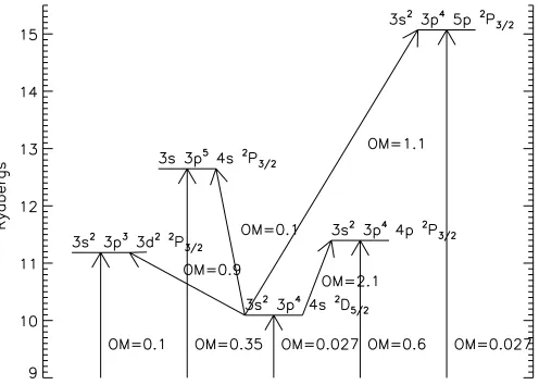
The outer region calculation includes exchange up to a total angular momentum quantum numberJ = 26/2. We have sup-plemented the exchange contributions with a non-exchange cal-culation extending fromJ=28/2 toJ=74/2. The outer region exchange calculation was performed in a number of stages. A coarse energy mesh was chosen above all resonances. The res-onance region itself was calculated with an increasing number of energies, as was done for the Iron Project Fexicalculation (Del Zanna et al. 2010).Pelan & Berrington(2001) suggested that a step in energy between 0.001 and 0.002 Ryd was sufficient to resolve the resonances. Here, the number of energy points was increased from 2000 up to 8000 (equivalent to a uniform step length of 0.0018 Ryd). We have then considered all the transi-tions from the ground state and calculated the maximum devia-tion between the various calculadevia-tions of the thermally-averaged collision strength. The results are shown in Fig.3.
Table 3.Level energies for Fex(n=3,4).
i Conf. Lev. Eexp Et Eb
1 3s23p5 2P
3/2 0.0 0.0 0.0
2 3s23p5 2P
1/2 0.143 0.141 (0.002) 0.143 3 3s 3p6 2S
1/2 2.636 2.681 (–0.045) 2.636 4 3s23p43d 4D
5/2 3.542 3.690 (–0.148) 3.531 (0.011) 5 3s23p43d 4D
7/2 3.542 3.691 (–0.149) 3.532 (0.010) 6 3s23p43d 4D
3/2 3.554 3.700 (–0.146) 3.541 (0.014) 7 3s23p43d 4D
1/2 3.568 3.714 (–0.145) 3.568 8 3s23p43d 4F
9/2 3.806 3.979 (–0.173) 3.806 (–0.000) 9 3s23p43d 2P
1/2 – 3.979 3.808
10 3s23p43d 4F
7/2 3.853 4.023 (–0.171) 3.853 11 3s23p43d 2P
3/2 – 4.054 3.880
12 3s23p43d 4F
5/2 3.889 4.058 (–0.169) 3.889 13 3s23p43d 4F
3/2 – 4.073 3.898
14 3s23p43d 4P
1/2 – 4.104 3.928
15 3s23p43d 2D
3/2 – 4.121 3.944
16 3s23p43d 4P
3/2 3.904 4.153 (–0.249) 3.975 (–0.071) 17 3s23p43d 4P
5/2 4.014 4.176 (–0.162) 4.014 18 3s23p43d 2F
7/2 4.017 4.195 (–0.178) 4.017 19 3s23p43d 2D
5/2 4.035 4.204 (–0.169) 4.035 20 3s23p43d 2G
7/2 4.111 4.305 (–0.194) 4.111 21 3s23p43d 2F
5/2 4.137 4.307 (–0.170) 4.123 (0.014) 22 3s23p43d 2G
9/2 4.108 4.311 (–0.203) 4.126 (–0.019) 23 3s23p43d 2F
5/2 4.393 4.573 (–0.180) 4.393 24 3s23p43d 2F
7/2 4.429 4.610 (–0.181) 4.429 25 3s23p43d 2D
3/2 – 4.904 4.697
26 3s23p43d 2D
5/2 4.704 4.946 (–0.242) 4.704 27 3s23p43d 2S
1/2 4.938 5.171 (–0.233) 4.938 28 3s23p43d 2P
3/2 5.141 5.512 (–0.371) 5.141 29 3s23p43d 2P
1/2 5.193 5.569 (–0.375) 5.193 30 3s23p43d 2D
5/2 5.221 5.581 (–0.359) 5.221 31 3s23p43d 2D
3/2 5.342 5.705 (–0.363) 5.342 35 3s 3p53d 4F
9/2 6.304 6.575 (–0.271) 6.304 (–0.000) 43 3s 3p53d 2F
7/2 6.719 6.931 (–0.212) 6.652 (0.068) 174 3s23p44s 4P
5/2 9.314 9.674 (–0.360) 9.308 (0.006) 179 3s23p44s 4P
3/2 9.383 9.743 (–0.361) 9.383 183 3s23p44s 2P
3/2 9.480 9.858 (–0.378) 9.480 192 3s23p44s 2P
1/2 9.558 9.940 (–0.382) 9.558 202 3s23p44s 2D
5/2 9.693 10.073 (–0.380) 9.696 (–0.003) 203 3s23p44s 2D
3/2 9.698 10.078 (–0.381) 9.698 229 3s23p44p 4P
5/2 10.192 10.564 (–0.372) 10.173 (0.019) 243 3s23p44p 4D
7/2 10.301 10.677 (–0.376) 10.283 (0.018) 266 3s23p44p 2F
5/2 10.588 10.969 (–0.381) 10.588 (–0.000) 267 3s23p44p 2F
7/2 10.623 11.013 (–0.391) 10.611 (0.012) 284 3s23p44p 2D
5/2 10.742 11.146 (–0.404) 10.742 (–0.000) 370 3s23p44d 2D
5/2 11.703 12.123 (–0.420) 11.693 (0.011) 374 3s23p44d 2D
3/2 11.711 12.132 (–0.420) 11.701 (0.010) 380 3s23p44d 4F
5/2 11.724 12.202 (–0.479) 11.770 (–0.046) 383 3s 3p43d2 2F
5/2 11.739 12.230 (–0.491) 11.797 (–0.058) 388 3s23p44d 2P
3/2 11.803 12.269 (–0.466) 11.835 (–0.032) 402 3s23p44d 2P
3/2 11.989 12.398 (–0.408) 11.961 (0.028) 407 3s23p44d 2P
1/2 12.005 12.420 (–0.415) 11.983 (0.022) 413 3s23p44d 2D
5/2 12.040 12.484 (–0.444) 12.040 415 3s23p44d 2D
3/2 12.056 12.491 (–0.436) 12.056 429 3s 3p54s 2P
3/2 – 12.642 12.199
452 3s23p44f 4F
9/2 12.652 13.092 (–0.439) 12.639 (0.013) 462 3s23p44f 4G
11/2 12.732 13.190 (–0.459) 12.732 (–0.000) 463 3s23p44f 4G
9/2 12.756 13.222 (–0.465) 12.756 467 3s23p44f 4G
7/2 12.847 13.262 (–0.416) 12.806 (0.041) 471 3s23p44f 2G
9/2 12.837 13.293 (–0.456) 12.837 (–0.000) 473 3s23p44f 4G
5/2 12.850 13.297 (–0.446) 12.840 (0.011) 488 3s23p44f 2F
7/2 12.957 13.385 (–0.428) 12.926 (0.031) 497 3s23p44f 2H
11/2 13.025 13.491 (–0.467) 13.025 (–0.000) 510 3s23p44f 2G
9/2 13.137 13.621 (–0.484) 13.157 (–0.020) 539 3s23p44f 2F
5/2 13.526 14.032 (–0.506) 13.559 (–0.033) Notes. The experimental level energies Eexp (in Rydbergs, from
Del Zanna et al. 2004, for then=3; andFawcett et al. 1972, forn=4)
[image:6.595.48.280.94.729.2]are shown, together with those obtained from our scattering targetEt and the adjusted ones,Eb. Values in parentheses indicate differences withEexp. Only a selection of levels is shown.
Fig. 3. Maximum relative difference (in percentage) between the thermally-averaged collision strengths from the ground state, calculated with an increasing number of energy points, from 2000 to 8000.
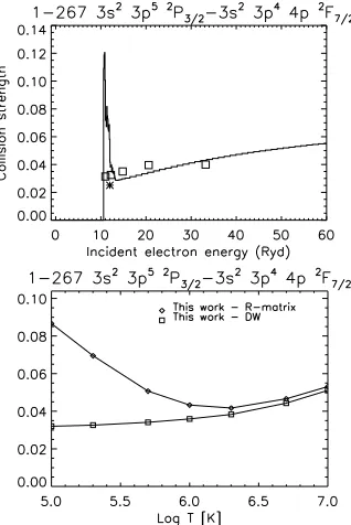
Fig. 4. Above: collision strength for the forbidden red coronal line, averaged over 0.1 Ryd in the resonance region. The data points are displayed in histogram mode. Boxes indicate the DW values. Below: thermally-averaged collision strengths, with other calculations.
intensity of the 1−5 line was underestimated by about 50%. The new atomic data remove the discrepancy.
[image:6.595.340.517.284.559.2]G. Del Zanna et al.: Atomic data for astrophysics: Fexsoft X-ray lines
[image:7.595.84.250.77.345.2]Fig. 5.Same as Fig.4, for the allowed 1−3 345.74 Å transition.
Fig. 6.Same as Fig.4, for the strong forbidden 1–5 257.26 Å transition.
temperatures. All other lines from the same transition array show a similar behaviour.
On the other hand, the strong forbidden transition from the ground state to the 3s 3p54s2P
3/2does not have much resonance
contribution, as we expected, i.e. the DW and R-matrix results are almost the same, as Fig.9 shows. The DW calculation of Malinovsky et al.(1980) is about a factor of two lower.
[image:7.595.354.514.379.628.2]As we expected, we find some resonance contribution for transitions to the 3s23p44p levels. Figure10shows an example
Fig. 7.Same as Fig.4, for the allowed 1–30 174.53 Å transition, the strongest in the EUV.
Fig. 8. Same as Fig. 4, for the allowed 94.012 Å transition. Note the strong enhancement due to the resonances. The asterisks are the
Malinovsky et al.(1980) calculations (DW and semi-classical).
of the excitation to a level producing one of the strongest lines (see Table1).
An enhancement is also present in the transitions to the 3s2 3p4 4d levels. Figure 11 shows one example, again for
[image:7.595.84.246.383.636.2]Fig. 9.Same as Fig.4, for the strong forbidden 1–429 transition. The asterisk is the DW value calculated byMalinovsky et al.(1980).
Fig. 10. Same as Fig. 4, for one of the important transitions to the 3s23p44p.
We then built ion population models with the DW excitation rates and the R-matrix ones, together with the same set of ra-diative rates. The relative intensities are shown in the first and third intensity columns of Table1. The effect of the resonances is obvious. The decay from the 3s23p44s2D
5/2is enhanced by
[image:8.595.92.251.381.619.2]almost a factor of two.
Fig. 11.Same as Fig.4, for one of the important transitions to the 3s2 3p4 4d. The asterisk is the DW value calculated byMalinovsky et al. (1980).
Fig. 12. Same as Fig. 4, for one of the important transitions to the 3s23p44f.
4.4. Including the n = 5, 6 levels
[image:8.595.349.519.390.647.2]G. Del Zanna et al.: Atomic data for astrophysics: Fexsoft X-ray lines
Fig. 13.The term energies of the target levels for the 62-configurations DW run (only 44 retained for the ion model).
44 configurations listed in Table4and displayed in Fig.13. The excitation rates and radiative data to/from then=5,6 levels have been merged with the previous R-matrix run. The level popula-tions were obtained, and the relative intensities for the selected lines are shown in Table1(RM+DW(n=6) model). We confirm the results ofMalinovsky et al.(1980), in that the inclusion of cascading fromn=5,6 levels increases the intensities of the de-cays from the 3s23p44s levels by about 20%, i.e. by a relatively
small amount.
Malinovsky et al.(1980) provided some estimates of the con-tribution from even higher levels, and from recombination from Fexi, however, they were even smaller.
4.5. The 3–429 3s 3p6 2S1/2–3s 3p54s2P3/2transition
As we have seen (cf. Fig. 9), the direct excitation from the ground to the 3s 3p5 4s2P
3/2is large, when compared to those
for the 3s23p44s levels. The 3s 3p54s2P
3/2level decays with a
strong dipole-allowed transition to the 3s 3p6 2S
1/2(3–429). The
resulting intensity as calculated with our most extended model is still larger than the 3s23p5 2P3/2–3s23p44s2D5/294.012 Å line.
The same is true at higher densities. It is somewhat puzzling that the main decays of the 3s23p44s levels were first identified by
Edlén(1937), but nobody has identified the stronger 3–429 line. We have run various DW calculations for other ions along the Cl-like sequence and for other sequences, and found the same types of transitions to be very prominent but not identified. We have found possible identifications, which will be presented in a separate paper.
For Fex, the 3–429 is the only line among all the decays from the 3s 3p5 4s levels to be easily detectable. The ab-initio
wavelength of then = 4 model is 91.5 Å. However, consider-ing the relative differences between experimental and ab-initio energies of the 3s2 3p4 4s and 3s23p4 4p levels, we estimated
that this line would fall around 95–96 Å.
We have searched extensively all experimental data, in par-ticular those B.C. Fawcett plates where transitions from the
Table 4.The target electron configuration basis and orbital scaling parametersλnlfor the 62-configurations DW run.
Configurations Scaling parameters
λnl
3s23p5 1s 1.41548
3s23p43d 2s 1.12358
3s23p44l(l=s, p, d, f) 2p 1.06501 3s23p33d2 3s 1.12476 3s23p33d 4s 3p 1.09729
3s 3p6 3d 1.11252
3s 3p53d 4s 1.21772
3s 3p54l(l=s, p, d, f) 4p 1.19803
3s 3p43d2 4d 1.20247
3s 3p43d 4l(l=s, p, d, f) 4f 1.35751
3p63d 5s 1.17511
3p64l(l=s, p, d, f) 5p 1.1442
3p53d2 5d 1.16260
3p53d 4l(l=s, p, d, f) 5f 1.28045 3s23p45l(l=s, p, d, f, g) 5g 1.41348 3s 3p55l(l=s, p, d, f, g) 6s 1.18612 3s23p46l(l=s, p, d, f, g) 6p 1.15788 3s 3p56l(l=s, p, d, f, g) 6d 1.18403 3p65l(l=s, p, d, f, g) 6f 1.30289 3p66l(l=s, p, d, f, g) 6g 1.37919 3s23p33d 4l(l=p, d, f)
3p64l(l=s, p, d, f) 3s 3p54l(l=d, f) 3s 3p43d 4l(l=s, p, d, f) 3p53d 4l(l=s, p, d, f)
Notes. The configurations below the line have been included in the CI expansion only.
3s23p44s feature prominently. We found only one candidate, an
[image:9.595.325.538.395.711.2]nearby 96.12 Å iron line, identified byEdlén (1937).Behring et al.(1972) also observed two strong lines of the same inten-sity at 96.007 and 96.119 Å, while in all other solar measure-ments (e.g.Manson 1972;Malinovsky & Heroux 1973) these lines are blended.
The only other line within a few angstroms is the 95.37 Å line. This is a self-blend of two decays from the 3s23p44s
lev-els, again identified by Edlén (1937). The combined inten-sity of these two lines at 1012 cm−3 is about the same as the 96.12 Å one, so the 95.37 Å cannot be further blended with the 3−429 transition.
We have carried out five increasingly large ab initio structure calculations just focussing on the 4s configurations. The idea was to calculate the energy difference between the 3s2 3p4 4s
4P
5/2and the 3s 3p54s2P3/2and then use the known energy of
the former to estimate the wavelength of the transition from the latter state to 3s 3p6 2S
1/2. The results of the five calculations, in
order of increasing complexity, are 91.97, 95.58, 95.78, 95.86, 95.89 Å. These are the result of purely ab initio calculations without empirical adjustments, and provide strong support for the identification of the 3–429 line with the iron 96.007 Å line.
5. Summary and conclusions
We have presented the first complete calculations forn=4,5,6 levels in Fex. The calculation of accurate atomic data for the n=4 levels has turned out to be quite complex and for the 3s2
3p44s, in particular, it required a large-scale R-matrix calcula-tion. Given the small collision strengths for excitations from the ground, these levels are mainly affected in two ways. First, the rates are increased significantly by strong resonances which are attached mainly to the 3s23p44p levels. Second, the population
of these levels is enhanced by cascading from higher levels, as already pointed out byMalinovsky et al.(1980).
It turns out that the previous calculation for the 3s2 3p44s levels, byMalinovsky et al.(1980), overestimated the collisional rates by about a factor of two. On the other hand, we found an increase of about a factor of two due to resonances. Resonances attached to higher levels not included in the present R-matrix calculations are not expected to make a large contribution. The intensity of the 94 Å as given with then=4 R-matrix data and cascading fromn=4,5,6 levels is only about 30% higher than currently calculated with CHIANTI.
We found that a large number of strong transitions are unidentified, as we saw in Feix(O’Dwyer et al. 2012). We have found strong evidence in support of the identification of the 3−429 3s 3p6 2S1/2−3s 3p54s 2P3/2 transition. We have found
many new tentative identifications. These will be discussed in a separate paper.
The issues highlighted here are quite general in the sense that they apply to other ions along the Cl-like sequence and to other
iron ions. Resonance contributions are important for many low-lyingn=4 levels, in particular for the 3s23pq4s levels. Decays from the 3s 3pq4s levels are strong but have not been previously identified. Work is in progress to address these issues.
Acknowledgements. G.D.Z. acknowledges the support from STFC via the Advanced Fellowship programme. We acknowledge support from STFC for the UK APAP network. B. C. Fawcett is thanked for his contribution in rescuing some of his original plates, and for the continuous encouragement over the years.
References
Aggarwal, K. M., & Keenan, F. P. 2005, A&A, 429, 1117 Aschwanden, M. J., & Boerner, P. 2011, ApJ, 732, 81 Badnell, N. R. 1997, J. Phys. B At. Mol. Phys., 30, 1 Badnell, N. R. 2011, Comp. Phys. Commun., 182, 1528
Badnell, N. R., & Griffin, D. C. 2001, J. Phys. B At. Mol. Phys., 34, 681 Behring, W. E., Cohen, L., & Feldman, U. 1972, ApJ, 175, 493
Behring, W. E., Cohen, L., Doschek, G. A., & Feldman, U. 1976, ApJ, 203, 521 Berrington, K. A., Eissner, W. B., & Norrington, P. H. 1995, Comp. Phys.
Comm., 92, 290
Brinkman, A. C., Gunsing, C. J. T., Kaastra, J. S., et al. 2000, ApJ, 530, L111 Burgess, A. 1964, Culham Conference on Atomic Collisions (AERE reprint 63) Burgess, A. 1965, ApJ, 141, 1588
Burgess, A. 1974, J. Phys. B At. Mol. Phys., 7, L364 Burgess, A., & Tully, J. A. 1992, A&A, 254, 436
Burgess, A., Chidichimo, M. C., & Tully, J. A. 1997, J. Phys. B At. Mol. Phys., 30, 33
Chidichimo, M. C., Badnell, N. R., & Tully, J. A. 2003, A&A, 401, 1177 Del Zanna, G. 2012, A&A, 537, A38
Del Zanna, G., Berrington, K. A., & Mason, H. E. 2004, A&A, 422, 731 Del Zanna, G., Storey, P. J., & Mason, H. E. 2010, A&A, 514, A40 Del Zanna, G., O’Dwyer, B., & Mason, H. E. 2011, A&A, 535, A46
Dere, K. P., Landi, E., Mason, H. E., Monsignori Fossi, B. C., & Young, P. R. 1997, A&AS, 125, 149
Edlén, B. 1937, Z. Astrophys., 104, 407 Edlén, B. 1942, Z. Astrophys., 22, 30
Eissner, W. 1998, Comp. Phys. Comm., 114, 295
Eissner, W., Jones, M., & Nussbaumer, H. 1974, Comp. Phys. Comm., 8, 270 Fawcett, B. C., Peacock, N. J., & Cowan, R. D. 1968, J. Phys. B At. Mol. Phys.,
1, 295
Fawcett, B. C., Kononov, E. Y., Hayes, R. W., & Cowan, R. D. 1972, J. Phys. B At. Mol. Phys., 5, 1255
Griffin, D. C., Badnell, N. R., & Pindzola, M. S. 1998, J. Phys. B At. Mol. Phys., 31, 3713
Grotrian, W. 1939, Naturwiss., 27, 214
Hummer, D. G., Berrington, K. A., Eissner, W., et al. 1993, A&A, 279, 298 Landi, E., Del Zanna, G., Young, P. R., et al. 2006, ApJS, 162, 261 Lemen, J. R., Title, A. M., Akin, D. J., et al. 2011, Sol. Phys., 172 Malinovsky, L., & Heroux, M. 1973, ApJ, 181, 1009
Malinovsky, M., Dubau, J., & Sahal-Brechot, S. 1980, ApJ, 235, 665 Manson, J. E. 1972, Sol. Phys., 27, 107
Mason, H. E. 1975, MNRAS, 170, 651
O’Dwyer, B., Del Zanna, G., Mason, H. E., Weber, M. A., & Tripathi, D. 2010, A&A, 521, A21
O’Dwyer, B., Del Zanna, G., Badnell, N. R., Mason, H. E., & Storey, P. J. 2012, A&A, 537, A22
Pelan, J. C., & Berrington, K. A. 2001, A&A, 365, 258 Petrini, D. 1970, A&A, 9, 392