A robust and efficient approach to detect 3D rectal tubes from CT colonography

City, University of London Institutional Repository

Citation

:

10.1118/1.3654842

This is the accepted version of the paper.

This version of the publication may differ from the final published

version.

Permanent repository link:

Link to published version

:

Copyright and reuse:

City Research Online aims to make research

outputs of City, University of London available to a wider audience.

Copyright and Moral Rights remain with the author(s) and/or copyright

holders. URLs from City Research Online may be freely distributed and

linked to.

City Research Online: http://openaccess.city.ac.uk/ [email protected]

A Robust and Efficient Approach to Detect 3D Rectal Tubes from CT Colonography

Xiaoyun Yang1,a) _{and Greg Slabaugh}1

Medicsight PLC, Kensington Centre, 66 Hammersmith Road, London,

UK

(Dated: 15 September 2011)

Abstract

Purpose: The rectal tube (RT) is a common source of false positives (FPs) in computer-aided detection (CAD) systems for CT colonography. A robust and efficient detection of RT can improve CAD performance by eliminating such “obvious” FPs and increase radiologists’ confidence in CAD.

Methods: In this paper, we present a novel and robust bottom-up approach to detect the RT. Probabilistic models, trained using kernel density estimation on simple low-level features, are employed to rank and select the most likely RT tube candidate on each axial slice. Then, a shape model, robustly estimated using Random Sample Consensus (RANSAC), infers the global RT path from the selected local detections. Subimages around the RT path are projected into a subspace formed from training subimages of the RT. A quadratic discriminant analysis (QDA) provides a classification of a subimage as RT or non-RT based on the projection. Finally, a bottom-top clustering method is proposed to merge the classification predictions together to locate the tip position of the RT.

Results: Our method is validated using a diverse database, including data from five hospitals. On a testing data with 21 patients (42 volumes), 99.5% of annotated RT paths have been successfully detected. Evaluated with CAD, 98.4% of FPs caused by the RT have been detected and removed without any loss of sensitivity.

Conclusion: The proposed method demonstrates a high detection rate of the RT path, and when tested in a CAD system, reduces FPs caused by the RT without the loss of sensitivity.

Keywords: Rectal Tube, RANSAC, CAD, eigenspace, CT colonography

I. INTRODUCTION

A. Motivation

Colorectal cancer is the second leading cause of cancer related death in western countries and the third most common human malignancy in the United States1. Most colorectal cancers arise from pre-malignant adenomatous polyps in the colon that develop into cancer over time. The progression from polyp to cancerous lesion takes more than ten years for most patients. Because of this slow growth rate, colorectal screening2 is an effective method for polyp detection, and subsequent removal reduces the risk of colorectal cancer by up to 90 percent3. Colonoscopy, the endoscopic examination of the colon using a flexible video camera, is the standard approach to colorectal screening; however, in recent years there has been much interest in CT Colonography (CTC), which uses CT images of the cleansed and insufflated colon4. Polyps can then be detected by a clinical reader who examines the CT data using advanced visualization software that provides both 3D endoluminal views of the colon as well as 2D multi-planar reformatted slices.

Although CTC has been demonstrated to be an effective colorectal screening approach5, it is possible for the clinical reader to fail to detect lesions, due to the large quantity of data generated (typically 800 - 2000 images per patient). Computer-aided detection (CAD) software assists the clinical reader by automatically analyzing the CT data and highlighting potential lesions. CAD may detect lesions that would have otherwise been missed by the reader, and may give the reader more confidence that lesions were not missed during the read. It has been demonstrated that the use of CAD leads to improvements in reader performance (at all levels of experience) in detecting lesions in CTC data6,7_.

CAD marks presented to the reader.

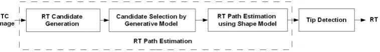
FIG. 1: Rectal Tube Detection Scheme.

Some research has been proposed9–11to address this problem. Iordanescuet al.9developed an image segmentation based method that detects, via template matching, the air inside the RT in the first nine CT slices, tracks the tube, and performs segmentation using morpho-logical operations. The template is generated in a fixed definition of shape. It is a relatively rigid method for detection, and may fail to take account of the shape variability by tracking 2D slices. It assumes that the RT can be detected by a set of fixed-shape template matching continuously during tracking, which could be too strong of an assumption. Suzuki et al.10 employed a Massive Training Artificial Neural Network (MTANN) to distinguish between polyps and FPs due to the RT. In the 73 patient data (146 volumes), MTANN detected all 20 RT FPs as well as 53 FPs due to other sources among the 224 FPs in total, without removal of any true positives. The method requires manual selection of representative train-ing samples. Imperfect selection of traintrain-ing samples could degrade the performance10_{. This} could introduce uncertainty to the performance. Barbuet al.11 _{designed a method to detect} the RT with the assumption that the RT can have large variable shape and appearance, which increased the complexity of their method. They first started detecting 3D circles using voting and Probabilistic Boosting Tree (PBT) methods, with a feature set consisting of 6720 features computed from gradient, curvatures, etc. A second classifier trained with PBT is used to detect short tubes from the detected 3D circles. Dynamic programming is employed to find the best RT segmentation from the detected parts.

B. Our contribution

a probabilistic model learned through kernel density estimation (KDE) on simple low-level features. With the rectal tube path robustly estimated, the RT tip is then estimated using a classifier trained on projection coefficients in an eigen-subspace of rectal tube subimages. The classifier provides a label for each axial slice if it contains the RT or not. From these outputs, a bottom-top clustering method merges the labels predicted by the classifier into a few major clusters, from which the position of the RT tip can be localized.

We note that this paper extends our preliminary work on RT detection presented in13 by inferring the RT tip location using the eigen-subspace, classifier, and clustering method mentioned above. Accurate tip estimation improves the FP detections per volume and reduces the likelihood that the method would produce a false negative when used in a CAD system to reduce false positives.

Our method is computationally inexpensive and reliable. The experimental results demonstrate a high detection rate in a diverse dataset, and when evaluated by a CAD system, achieve a good reduction of FPs caused by the RT without any loss of sensitivity.

II. METHODS

A. Overview

We present a learning framework to combine probabilistic models for low level detection of the air in the rectal tube with a global shape model of the RT path. The overview of the system is presented in Figure 1.

We start with simple image processing, applied to each 2D axial slice, to detect air regions (RT candidates) within the body in the most caudad slices, starting at the anal verge and moving up the abdomen towards the lungs. For each RT candidate, three simple low level features are computed: the normalized spatial position xand y of the centroid and the size h of the region.

(a) (b)

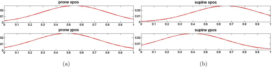
FIG. 2: The probability distributions of normalized candidate position x-direction, y-direction. (a) supine, (b) prone.

KDE predictions. We have two assumptions in this paper. First, the spatial distribution of the RT within the body can be approximately described by a probabilistic model built from training data. Intuitively, this assumes that the candidate is more likely selected if its position is close to the mean position of training samples. With an additional constraint that the RT must located within or near the colon mask, we can further remove the bad (false) candidates if a colon mask is provided. Second, the RT is a possibly bent cylindrical structure placed on the bottom of body. With this knowledge, by seeking a quadratic path supported by maximum number of candidates, we can differentiate good candidates and bad ones selected by the probabilistic model. The RT path can thus be estimated from good candidates.

Once the RT path is located, we search for the RT tip with a prior knowledge that the RT is less than 140mm in the body. Firstly, for each slice, centering around the path point at that slice, a set of 2D sub-images is extracted and projected into a eigen-subspace; and a quadratic discriminant classifier is applied on the projected subspace to make the RT/non-RT prediction; a bottom-up clustering approach is then proposed to apply on those predictions to merge them iteratively into a small number of clusters, the position of the RT tip can then be located. The details are discussed in the following subsections.

B. Probabilistic models for 2D candidate detection of RT regions

(a) (b) (c)

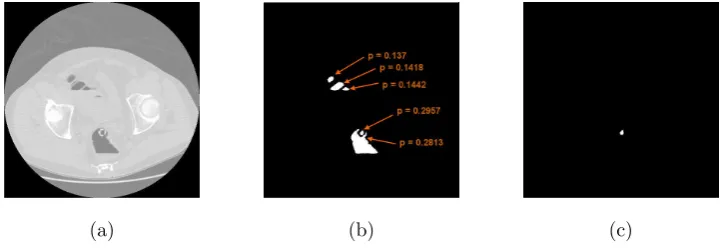
FIG. 3: Examples of the candidate selected by KDE. (a) the CT image, (b) the candidate regions, and (c) the region selected by KDE. This region corresponds to the air in the RT.

for selection of the most probable candidate on a given slice.

The air region in the RT can be identified on an axial image slice using standard im-age processing techniques. For each slice, we apply simple thresholding using a threshold value ranged between [−700,−850]9,14_{, e.g. −750 HU. All the air pixels then belong to the} background and all the remaining pixels are assigned to the foreground pixels; the largest foreground region is morphologically filled and then regarded as the body region at that slice. The air regions located within this body region are then kept as inside-body air and the others are discarded as outside-body air. A 3D minimum bounding box rect to enclose all the 2D body regions can be uniquely determined with simple boolean min or max opera-tions on the x-y-z coordinates of all the pixels in body regions, where the x-y-z coordinates of the bounding box is denoted to be (rectx1, rectx2, recty1, recty2, rectz1, rectz2).

Each candidate is represented by its centroid (Ci

x, Cyi, Czi). Three low level features, (V_xi, V_yi, V_si), for each candidate are computed: the normalized spatial position (V_xi) and (Vi

y) in the xand ydirection, and the region size (Vsi). The normalized spatial positions are determined as Vi

candidates to have area in the range [0.5,130]mm2_{, which we set empirically. A kernel} density function (KDE) can be built by summing a set of kernels15_{with the selected feature} data (Vi

x, Vyi, Vsi), as shown in Equation 1. From the constructed KDE, the probability of a given candidate V being RT can be estimated as

P(RT|V) =

         1 T ∑N i=1e

−(Vx−V i_x)2 2h2_x ∑n

i=1e

−(Vy−V iy)2 2h2y

if Vs ∈[0.5,130]mm2 0 otherwise

(1)

where P(RT|V) represents the probability of a given candidate being RT, (Vx, Vy, Vs) is the feature vector of the candidate V. (Vi

x, Vyi, Vsi) (i = 1, .., N), as defined earlier, is the ith example used for training. If Vs is too big or too small, a penalty is given and the probability is zero, and T is a normalization factor so that the probability sums to 1. The KDE model is generated from prone and supine data separately using Gaussian kernels with bandwidth hx, hy inx and y direction with value 0.25 for both. In this function, each data point has a contribution to the probability controlled by a Gaussian function. Figure 2 gives the probability distributions of normalized spatial position of RT for prone and supine respectively. With a large bandwidth value, the distribution behaves as a single Gaussian, where the candidates located near the center of body are more likely to be selected than the candidates at the border of body, particularly in thex-direction. In the y-direction, the RT candidates at the supine position are located relative closer to the bottom than the ones at the prone position. These reflect the anatomical knowledge of the RT position in the CT scan.

In the testing stage, we apply the appropriate (prone or supine) probabilistic model to the candidate’s feature vector. A probability can then be estimated for each RT candidate. The candidates are ranked by the estimated probability and only the one with the maximum probability in each slice will be selected. Figure 3 (a) shows an example CT image, (b) the candidate regions and (c) most likely candidate selected by the KDE model.

(a) (b)

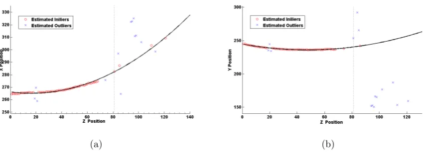
FIG. 4: Examples of RANSAC fitting for two volumes data in the xz and yz planes. Red circles represent inliers, blue crosses represent outliers, the black dotted line is the fitted

path using RANSAC, and the black dotted line indicates the end of the RT.

C. RT path estimation using a global shape model

In this subsection we describe how the underlying RT path is inferred from the RT candidate centroids selected in the previous step.

The RT is a cylindrical tube placed in the patient’s colon, and once the colon is insufflated with room air and there is no force to twist the RT. The path of the RT can be approximated as a quadratic curve (which includes a straight line as a special case). While there may occasionally be some other air-filled structure or noise giving a quadratic path, the RT is easily identified as the longest path along a smooth and continuous quadratic curve starting at the bottom of the patient. To estimate the correct RT path, one must differentiate the outliers from the inliers that represent the true locations of the RT. From the inliers, we can infer the other 2D RT locations missed by KDE. With the prior model of the global shape information that the RT path is a quadratic curve and continuously appears in the most caudad slices, we use that as a criteria to seek a maximum set of inlier points that can fit the quadratic curve which can be resolved by RANSAC12_{, as shown in Equation 2:}

ˆ

θ = arg max θ

n

∑

i=1

f(e2_i|θ) (2)

where

f(e2_i|θ) =

  

1 e2 i < δ2 0 otherwise

(3)

where θ is the quadratic model to be estimated, ei is the error or the distance between the data Vi and the estimated curve. δ is a threshold under the hypothesis that the error is generated by a true inlier contaminated with a Gaussian noise P[ei ≤δ], where we expect the value ofP is 0.95. The estimation of 3 parameters for a quadratic curve requires 3 points at least; and RANSAC adopts a random selection process to choose any 3 points to estimate a quadratic model θ, this process is repeated k times. And the one with the maximum number of inliers shown in Equation 2 is chosen. Let Pk be probability that the points selected to estimate the model are all inliers (n is total number of selected points). pis the probability that any selected point is inliers (p= numberof inliersindata_{numberof pointsindata}). Their relationship can be characterized as follows12_:

the required number of trials is

k = log(1−Pk)

log(1−pn₎ (5)

From Equation 5, assuming that the percentage of inliers in the data is p= 0.5, and we know the required number of points for the estimation of quadratic model is 3 (n = 3), to attain a 0.99 probability of success (Pk = 0.99), it only requires only 35 (k=35) times to repeat this process, which can be computed quickly.

A 3D space curve quadratic in z models the path as [Cx(z), Cy(z), z]T = [θ0x+θ1xz + θ2xz2, θ0y +θ1yz +θ2yz2, z]T, where the estimation of [θ0x, θ1x, θ2x] and [θ0y, θ1y, θ2y] is per-formed separately in the xz and yz planes respectively using RANSAC.

As shown in Figure 4, the black line illustrates the inferred RT path from the inliers (red circles). Even in the presence of large outliers (non-RT locations), the estimated RT path estimated by RANSAC is quite reliable. After RANSAC fitting, given a slice number, we can predict the RT path location. RANSAC can be viewed as a method to achieve a robust regression to fit the global shape model to data containing outliers.

D. RT Tip Detection

In this subsection we describe how to efficiently detect the RT tip along the RT path given by the previous step.

1. Eigentubes: Eigenspace of the RT

Kirby and Sirovich17_{first proposed to represent an arbitrary face with a set of eigenvectors} using principal component analysis. Turk and Pentland18 further developed this idea to construct a fast matching algorithm to recognize the face with the coefficients of eigenfaces. Under a much smaller subspace constructed by the first few eigenvectors, the classification of new samples by computing its distance to the training samples of different classes can be efficiently solved. We propose to use such an eigen-picture method for the detection the RT region along the estimated path, forming a subspace of RT images we call eigentubes.

(a) (b) (c) (d) (e) (f) (g) (h) (i)

(j) (k) (l) (m) (n) (o) (p) (q) (r)

FIG. 5: Eigentubes: the images of the first 18 eigenvectors.

on each position (Cx+{−5,0,5}, Cy +{−5,0,5}, Cz). Thus, we gathered in total of 9 sub-images for each given location (Cx, Cy, Cz). We then have a set of representative images with a [ ˆx⃗1, ..., ˆx⃗n], where the image ˆx⃗i is a d×1 dimension vector (d = r×c, r (r = 21)) represents the number of rows and c (c = 21) represents the number of columns of the 2D image) formed by appending each row of the image into the vector sequentially. Any image can be represented in such a form:

⃗

xi =Uqλ⃗i (6)

and

⃗

xi = ˆx⃗i−⃗µ (7)

where⃗µ(dimensiond×1) is a mean image of the set images, x⃗i is the observation of data ˆx⃗i centered at ⃗µ. We define a matrix X = (x⃗1... ⃗xn), where x⃗i is the ith column of the matrix. To best represent the n images of this set X, each of the image is d×1 dimension with a much smaller dimensionq, the problem of seeking such subspace is formulated as minimizing the reconstruction error:

Uq= arg min Uq

n

∑

i=1

∥x⃗i−Uqλ⃗i∥ (8)

(q×1) is a vector of coefficients, and this can be obtained by projectingx⃗i onto the subspace defined by Uq. Since the column of Uq is orthogonal, the coefficients can be obtained by using product of each basis vector with x⃗i,⃗λ = UqTx⃗i, Equation 8 can then be represented as:

Uq = arg min Uq

n

∑

i=1

∥x⃗i−UqUqTx⃗i∥ (9)

where UqUqT acts as a projection matrix and maps each image x⃗i into its rank q. This can be solved by a singular value decomposition of X:

Xq =UqΣVT

where Xq is the approximate representation of X using the first q eigenvectors; Uq is d×q matrix, the column of Uq is a eigenvector of XXT, Σ is a diagonal matrix, the value is its square of eigenvalue in a decreasing order to the covariance matrix XXT. The first eigenvector of covariance XXT _{can be intuitively explained as the direction that the data} set has maximal variance.

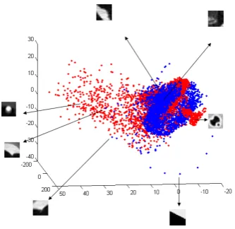
FIG. 6: PCA (3D) mapping of 2D candidate image for RT, red dots represent RT candidate, blue dots represent non-RT candidates.

2. Classification and Clustering

In the constructed eigenspace, each sub-image is represented as a data point. Quadratic discriminant analysis (QDA) is applied on the eigen-subspace for the detection/classification of the RT. Figure 7 illustrates a 5-fold validation result by projecting into a different number of subspace dimensions. We use the first 17 eigenvectors to construct the subspace since there is no clear additional gain in the performance with more dimensions.

FIG. 7: RT classification, 5 fold cross validation.

(a) (b) (c)

(d) (e) (f)

FIG. 8: Examples of detected RTs scanned from three hospitals, (a-b), (c-d), (e-f) are from the same hospital respectively.

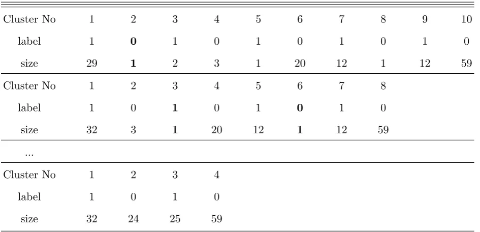
TABLE I: A table demonstrating grouping process.

Cluster No 1 2 3 4 5 6 7 8 9 10

label 1 0 1 0 1 0 1 0 1 0

size 29 1 2 3 1 20 12 1 12 59

Cluster No 1 2 3 4 5 6 7 8

label 1 0 1 0 1 0 1 0

size 32 3 1 20 12 1 12 59

...

Cluster No 1 2 3 4

label 1 0 1 0

size 32 24 25 59

algorithm is shown in Figure 9.

FIG. 9: Pseudocode of the RT clustering.

III. RESULTS

The data are collected from five institutions. CT images were generated using scanners from all the major manufacturers, including Siemens, GE, Philips, and Toshiba, with 4, 8, 16, 32, and 64 multi-slice configurations, KVp ranged from 120 −140, and exposure ranged from 29 - 500 mAs. All subjects were scanned within the years between 1999 and 2008, and roughly 80% were administered fluid and fecal tagging. The RTs from those data were manufactured by Bracco and VMPAP, with or without hemispherical tip. The diameter ranged within 6−11mm, the maximum intensity of the RT wall can be 550HU approximately, and the maximum intensity at tip position can be approximately 3072.

(white circle), rendered directly through the gray-scale image.

Our second experiment evaluates the RT detection for suppression of FPs in CAD. Any detection by CAD is removed as a FP if the distance between the center of the detected region and the center of the detected RT is less than 10mm in-plane and 7mm out-of-plane. On the 42 volume testing datasets, we could reduce 119 FPs generated by CAD (RT filtering is turned off)8, and the average FPs per volume is reduced to 5.3 from 8.3, which is 35.6% of improvement in FP reduction, without any loss of sensitivity. We repeat this RT filtering but by replacing the estimated RT position with the annotated RT position, where 121 FPs can be removed in total, including the 119 FPs identified by our approach and with only 2 additional missed FPs. This shows that our approach has detected 98.4% of FPs caused by the RT and didn’t remove any CAD mark from other sources, particularly true positives. In our data, we have found no true positives touching the RT and therefore no sensitivity loss due to this reason. The approach proposed in 11 _{was tested on a 210} datasets, achieving 94.7% detection rate and removing additional 26 CAD marks caused by other sources. Although the data set is different and our testing dataset is smaller, our performance has shown a very competitive performance in removing RT FPs and keeping the CAD sensitivity. We attribute the improved results of our method to the global shape model, which provides robustness to potentially erroneous local features.

IV. DISCUSSION

The method proposed in9 determined a path by the first nine air hole regions. Tracking a long path, the RT can be detected using template matching with a set of fixed shape templates. The method is relatively rigid for detection, and may fail to take account of the shape variability when tracking 2D slices. The assumption that the RT can be continuously detected by a set of fixed-shape template matching during tracking could be very strong and may lead to incorrect or partly detection only. Indeed, in our work we have noticed that local detections can be erroneous on individual slices, thereby suggesting a more global approach achieved through the shape model in our approach. The method proposed by Barbu et al.11 made a very weak assumption that the RT path can be any curved shape, which we believe underconstrains the problem and introduces additional complexities into the algorithm, such as two level PBT training. In11 a large feature set is required for the task of classification, e.g. approximate 6720 features for circular region detection in PBT. In this paper, we assume the path of RT to be a straight line or quadratic curve given that the knowledge that the RT exhibits a slight bending or straight-like shape inserted into the rectum of the body, matching observation in practice. Our experiments demonstrate the effectiveness of this assumption by giving a high detection rate of the RT in our data collected from different sources. This simplifies the complexity of our algorithms and requires only 3 simple low level features to be computed: 2D normalized positions (x,y) and the size of air regions.

We have tested this approach on the image without RT. When the input image does not have RT, the estimated path is not on the RT path. Searching along the path, most extracted sub-images don’t have the appearance of RT tip. After tip classification and clustering stage, the tip detector is going to end at the staring slice 0. This correctly reflects the fact that there is no RT in the image.

with an eigentube method. A QDA classifier is applied to the transformed 17-eigenvectors constructed subspace. Each 2D sectional image of RT can be projected into a data point in this subspace. In the subspace, the similar appearance object is much closer to each other than the very dissimilar appearance ones. This allows some degree of variance in the appearance among the samples from RT candidates. The classification only requires the computation of the data points distribution in this subspace, which is quite cost-effective. We design a bottom-up clustering method to have a high-level view of the individual local detections on each section, with which an optimal decision to determine the place of the RT tip can be made.

Our method is designed generally to be robust from outlier data’s influence. However, the accuracy of tip detector relies on the training samples to be representative. The RT path should generally pass through axial section perpendicularly or with a large angle with the axial plane. Some extreme cases that the angle between RT path and axial section could be small, the image of the intersection and axial plane may look very different from training sample images. In these cases, the eigentube detector may fail to accurately detect the tip. However, in practice, we have not observed cases where the detection failed due to this reason.

The balloon inflated at the top of the RT can be another potential source of FPs. Due to partial volume effect, there is not a clear boundary of the balloon, which makes its detection difficult. Our future work will try to estimate the balloon position using the estimated RT path and reduce the balloon’s resulting FPs.

V. CONCLUSIONS

shown a state-of-the-art performance in detecting the RT path and removing FPs resulting from the RT in our CAD system.

REFERENCES

1_{“Cancer facts and figures,” American Cancer Society Annual Report 12, 11–12 (2007).} 2_{M. E. Zalis, M. A. Barish, J. R. Choi, A. H. Dachmann, H. M. Fenlon, J. T. Ferrucci, S. N.}

Glick, A. Laghi, M. Macari, E. G. McFarland, M. M. Morrin, P. J. Pickhardt, J. Soto, and J. Yee, “CT colonography report and data system: A consensus proposal,” Radiology

236, 3–9 (2005).

3_{S. Winawer, “The achievements, impact, and future of the national polyp study,”} Gas-trointest. Endosc. 64, 975–978 (2006).

4_{C. D. Johnson and A. H. Dachman, “CT Colonography: The next colon screening} exami-nation?” Radiology 216, 311–319 (2000).

5_{C. D. Johnson, M. Chen, A. Toledano, J. Heiken, A. H. Dachman, M. D. Kuo, C. Menias,} B. Stewert, J. I. Cheema, R. G. Obregon, J. L. Fidler, P. Zimmerman, K. M. Horton, K. Coakley, R. B. Iyer, A. K. Hara, R. A. Halvorsen, G. Casola, J. Yee, B. A. Herman, L. J. Burgart, and P. J. Limburg, “Accuracy of CT colonography for detection of large adenomas and cancers,” N. Engl. J. Med. 259, 1207–1217 (2008).

6_{D. Burling, A. Moore, M. Marshall, J. Weldon, C. Gillen, R. Baldwin, K. Smith, P.} Pick-hardt, L. Honeyfield, and S. Taylor, “Virtual colonoscopy: effect of computer-assisted detection (CAD) on radiographer performance,” Clin. Radiol. 63, 549–556 (2008).

7_{E. M. Lawrence, P. J. Pickhardt, D. H. Kim, and J. B. Robbins, “Colorectal polyps:} Stand-alone performance of computer-aided detection in a large asymptomatic screening population1,” Radiology 256, 791–798 (2010).

8_{G. Slabaugh, X. Yang, X. Ye, R. Boyes, and G. Beddoe, “A robust and fast system for} CTC computer-aided detection of colorectal lesions,” Algorithms 3, 21–43 (2010).

9_{G. Iordanescu and R. M. Summers, “Reduction of false positives on the rectal tube in} computer-aided detection for CT colonography,” Med. Phys. 31, 2855–2862 (2004). 10_.

12_{M. A. Fischler and R. C. Bolles, “Random sample consensus: a paradigm for model fitting} with applications to image analysis and automated cartography,” Commun. ACM 24, 381–395 (1981).

13_{X. Yang, G. Beddoe, and G. Slabaugh, “Learning to detect 3D rectal tubes in CT} colonog-raphy using a global shape model,” in MICCAI Virtual Colonoscopy Workshop (2010) pp. 61–66.

14_{P. Lia, S. Napel, B. Acar, D. S. Paik, R. B. Jeffrey, and C. F. Beaulieu, “Registration of} central paths and colonic polyps between supine and prone scans in computed tomography colonography: pilot study,” Med. Phys. 31, 2912 (2004).

15_{A. Bowman and A. Azzalini, Applied smoothing techniques for data analysis: the kernel} approach with S-Plus illustrations, Vol. 18 (Oxford University Press, USA, 1997).

16_{P. Soille, Morphological Image Analysis: Principles and Applications, 2nd ed.} (Springer-Verlag New York, 2003).

17_{M. Kirby and L. Sirovich, “Application of the karhunen-loeve procedure for the} character-ization of human faces,” IEEE Trans. Pattern Anal. Mach. Intell. 12, 103–108 (1990). 18_{M. Turk and A. Pentland, “Eigenfaces for recognition,” J. Cognitive Neurosci. 3, 71–86}

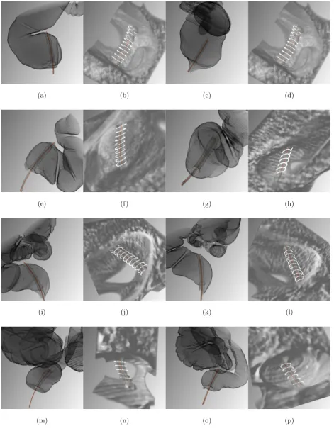
(a) (b) (c) (d)

(e) (f) (g) (h)

(i) (j) (k) (l)

(m) (n) (o) (p)

FIG. 10: The visualization of RT detection. Each row shows a patient respectively, the first two (prone position) and the last two (supine position). The first and third column illustrates the estimated RT path (red line), rendered directly through a segmented colon.