Distributed Optimal Lexicographic Max-min Rate Allocation in Solar
Powered Wireless Sensor Networks
Shusen Yang and Julie McCann, Imperial College London
Understanding the optimal usage of fluctuating renewable energy in Wireless Sensor Networks (WSNs) is complex. Lexicographic Max-min (LM) rate allocation is a good solution, but is non-trivial for multi-hop WSNs, as both fairness and sensing rates have to be optimized through the exploration of all possible forwarding routes in the network. All current optimal approaches to this problem are centralized and off-line, suffering from low scalability and large computational complexity; typically solving O(N2) linear
programming problems for N-node WSNs. This paper presents the first optimal distributed solution to this problem with much lower complexity. We apply it to Solar Powered WSNs (SP-WSNs) to achieve both LM optimality and sustainable operation. Based on realistic models of both time-varying solar power and photovoltaic-battery hardware, we propose an optimization framework that integrates a local power management algorithm with a global distributed LM rate allocation scheme. The optimality, convergence, and efficiency of our approaches are formally proven. We also evaluate our algorithms via experiments on both solar-powered MicaZ motes and extensive simulations using real solar energy data and practical power parameter settings. The results verify our theoretical analysis and demonstrate how our approach outperforms both the state-of-the-art centralized optimal and distributed heuristic solutions.
Categories and Subject Descriptors: C.2.2 [Computer-Communication Networks]: Network Protocols
General Terms: Design, Algorithms, Theory, Performance
Additional Key Words and Phrases: Solar Powered Wireless Sensor Networks, Power Management, Lexico-graphic optimality, Distributed multi-objective optimization, Max-min fairness
1. INTRODUCTION
The top two challenges facing wireless sensor networks (WSNs) are that of network-wide longevity and maintenance after deployment. The ability to conserve energy is core to both these challenges. Therefore harvesting energy from the environment brings a step change that ensures the viability of WSN for real world deployments [Sudevalayam and Kulkarni 2011; Sharma et al. 2009]. However, the ability of the WSN to meet their requirements while maximizing longevity will be compromised if the system is not able to exploit renewable energy optimally. Various environmental energy sources exist, such as solar, thermal, wind and vibrational. Of these, solar energy has been more widely considered and Solar Pow-ered WSNs (SP-WSNs) have been attracting a growing interest in various research fields including hardware system design (e.g. [Taneja et al. 2008]), node-centric power manage-ment schemes (e.g. [Kansal et al. 2007]), as well as network-wide algorithms (e.g. [Liu et al. 2011]).
Renewable solar energy provides an opportunity to achieve so-called Energy Neutral Operation (ENO) [Kansal et al. 2007]; that is, the solar-powered node achieves theoretically perpetual operation ( it always has energy). The main power management goals for solar-powered sensor nodes, therefore, are to achieve both ENO while maximizing capacity or
Author’s addresses: Shusen Yang and Julie McCann, Department of Computing, Imperial College London. Permission to make digital or hard copies of part or all of this work for personal or classroom use is granted without fee provided that copies are not made or distributed for profit or commercial advantage and that copies show this notice on the first page or initial screen of a display along with the full citation. Copyrights for components of this work owned by others than ACM must be honored. Abstracting with credit is permitted. To copy otherwise, to republish, to post on servers, to redistribute to lists, or to use any component of this work in other works requires prior specific permission and/or a fee. Permissions may be requested from Publications Dept., ACM, Inc., 2 Penn Plaza, Suite 701, New York, NY 10121-0701 USA, fax +1 (212) 869-0481, or [email protected].
c
⃝YYYY ACM 0000-0000/YYYY/01-ARTA $10.00
workload, rather than to simply maximize their lifetime (e.g. [Moser et al. 2010; Niyato et al. 2007]). To facilitate this, both the time-varying nature of solar power and the behaviors of photovoltaic-battery hardware system (e.g. battery recharging inefficiencies) should be realistically modeled.
In SP-WSNs, each senor node collects environmental data then forwards sensor data to a sink, or to multiple sinks, in a multi-hop fashion. Besides ENO at each sensor node, SP-WSNs aim at achieving the following two nework-wide objectives: (1) high network throughput for better solar energy resource utilization; (2) fair sensing rate assignment for all nodes across the network. However, there is a fundamental trade-off between network throughput and fairness for given solar energy resources. On one hand, if we only maximize network throughput, the sensors that are farthest from the sinks, or those which have poor solar harvesting opportunities, will be allocated much lower sensing rates than those closer to the sink, resulting in potentially unacceptable bias in the readings coming from network. On the other hand, absolute fairness (i.e. enforce equal sensing rates for all nodes) would lead to significant reduction in network throughput and inefficient solar energy usage (e.g. energy may be lost due to the battery overcharging).
Max-min fairness [Bertsekas and Galager 1992] is a well-recognized approach to balance the tradeoff between network throughput and fairness, and is widely adopted in rate al-location and control schemes in WSNs [Liu et al. 2011; Rangwala et al. 2006; Sridharan and Krishnamachari 2009]. In the context of WSNs, we describe a sensing rate allocation as max-min fair if no sensor can be allocated a higher rate without reducing the rate of another sensor that has equal or lower rate. Classic max-min rate allocation assumes that underlying end-to-end data traffic routes [Bertsekas and Galager 1992; Liu et al. 2011; Rangwala et al. 2006; Sridharan and Krishnamachari 2009] are predetermined, and purely adjusts the sens-ing rates at the transport layer. Therefore, there exists a huge number of classic max-min rate allocations for a given network, because the number of all possible underlying routes is of exponential order of the number of nodes in the network.
In this paper, we focus on a generalization of max-min rate allocation, the Lexicographic Max-min (LM) rate allocation [Chen et al. 2007; Hou et al. 2008; Liu et al. 2011; Radunovic and Boudec 2007], for SP-WSNs with arbitrary topologies. LM rate allocation jointly opti-mizes the end-to-end routes and the sensing rate allocation at the network and transport layers respectively, i.e. it computes the optimal max-min rate assignment by exploring all possible routes and energy resources in SP-WSNs. Therefore, LM rate allocation is optimal over all possible classic max-min allocations for a given network.
Theoretically, it is proven that the LM vector isuniquely optimal over any given convex and compact set [Radunovic and Boudec 2007]. This means that as long as the network con-straints (energy in SP-WSNs) form an unique convex and compact set for all possible rate allocations, the LM rate allocation will be the unique optimal solution. To compute the LM vector, an approach called max-min programming is proposed in [Radunovic and Boudec 2007]. All current optimal solutions [Chen et al. 2007; Hou et al. 2008; Liu et al. 2011] to the LM rate allocation problem in WSNs can be considered as specific implementations of the max-min programming approach. However, all these solutions are centralized and suf-fer from a large computational complexity; of the order of solvingN2 Linear Programming (LP) problems for aN-node WSN. Therefore, although they are solvable in polynomial-time, their centralized nature and complexity still prohibits their use in practical applications. Furthermore, such centralized approaches may lead to loops in the computed routes as-sociated with the LM rate allocation, leading to large end-to-end delays and unnecessary network resource costs.
acyclic graphs (DAG, i.e. multi-path routing) respectively. Furthermore, both of them are designed only for WSNs with a single sink, which restricts their application in large-scale WSNs where multiple sinks exist (e.g. [Shah-Mansouri et al. 2009]). In contrast, LM rate allocation considers all possible routes over arbitrary network topologies with either a single sink or multiple sinks. To the best of our knowledge, there exists no distributed solution to LM rate allocation problem yet.
In this paper, we focus on fully distributed solution to the LM rate allocation. In doing so, we demonstrate that designing a distributed solution for LM rate allocation is much more difficult than the traditional distributed Network Utility Maximization (NUM)-based rate control scheme; well-studied over the past decade [Chiang et al. 2008]. The core reason for this is that LM rate allocation is inherently a multi-objective optimization problem (e.g. [Huang 2007; Salles and Barria 2008]), while NUM-based rate control algorithms normally solve single-objective convex optimization problems only (i.e. they typically maximize ag-gregated concave utility functions such as α-fairness [Mo and Walrand 2000; Lan et al. 2010]).
The main contributions of this paper are summarized as follows:
(1) We present a systematic approach to LM rate allocation in SP-WSNs with arbi-trary topologies and multiple sinks (or a single sink). This is formalized as a joint power management, routing, and rate allocation problem. The formalization considers both the time-varying nature of the solar power and realistic photovoltaic-battery hardware behav-iors; such as battery capacity, recharging inefficiencies, and energy leakage. We decompose the formalized problem into two sub-problems: a LP problem for Local Power Management (LPM) that optimizes power for each node, and a multi-objective optimization problem for the network-wide LM rate allocation.
(2) An efficient Local Power Management (LPM) algorithm is proposed to compute the maximum feasible energy consumption budget for each sensor node to ensure ENO. Com-pared with solving LP at runtime, our LPM algorithm remains optimal with a much lower complexity (similar to a sorting operation), which is suitable for sensor nodes with limited computation resources.
(3) We develop the first distributed optimal approach to the global LM rate allocation problem. It operates by iterating through two distributed algorithms: a dual-decomposition-based algorithm, namely the Distributed Maximum Common Rate (DMCR) and the LM rate Determination (LMD); a graph-theoretic scheme. Our DMCR-LMD approach is not only fully distributed, but also achieves a worst-case complexity ofO(N) LPs to compute LM rate allocation for aN-node SP-WSN, which is much more efficient than current centralized approaches requiringO(N2) LPs.
(4) We present theoretical proofs of the optimality, convergence, and efficiency for both the individual algorithms and the whole system. Furthermore, we also demonstrate several nice properties of our approaches such as the loop-free optimal routing with respect to the LM rate allocation.
(5) The LPM algorithm is evaluated on a solar-powered MicaZ mote. Using a realistic power model and parameter settings, we also constructed simulations to evaluate the per-formance of our DMCR-LMD approach, in terms of optimality, overheads, convergence, and scalability. Simulation results verify our theoretical analysis and demonstrate that our approach manages to achieve much better fairness than the state-of-the-art distributed al-gorithms DLEX and DLEX-DAG, and with much lower complexity compared with the centralized approaches. In addition, we also study important practical issues such as how to overcome errors in solar power prediction to ensure ENO for realistic scenarios, through LPM parameter adjustments.
algorithms. In Section 7, we discuss practical issues of implementing DMCR-LMD approach in real SP-WSNs. The evaluation of our approach is presented in Section 7. Section 8 discusses the related work and we finally we conclude the paper in Section 9.
2. SYSTEM MODEL
We consider a multi-hop SP-WSN that consists of several sensor nodes, and one or multiple sinks. The SP-WSN can be represented as a directed graph G(V ∪ S,L) whereV is the set of all sensor nodes, S is the set of all sinks, andL is the set of all logical links. For each node x∈ V ∪ S, define Nxas the set of all one-hop neighbors ofxexcludingx.
Sensor nodexcollects environmental data (e.g. temperature and humidity) at a sensing raterx≥0. A data packet is sent in a multi-hop manner to any sink inS. Letfx,y ≥0 be the transmission rate at which node xtransmit sensor data to nodey, (x, y)∈ L.
2.1. Energy Model
δ η
Fig. 1. Prediction interval and energy flow.
To model the time-varying solar power, time is divided into identical discrete slots with duration δ(e.g. [Challen et al. 2010; Moser et al. 2010]). Due to the predicability of solar power, a prediction algorithm (e.g. [Bergonzini et al. 2010]) is assumed to be used to estimate the harvesting profile of every non-overlapping prediction interval consisting of L slots, as shown in Figure 1 (a). At the beginning of every prediction interval, harvested energyhi
xin every future sloti∈Iis estimated, whereI={1, 2, ..., L}. Based on the predicted harvesting profile of every prediction interval, our distributed algorithms calculate the optimal LM rate allocation and corresponding routes for this prediction interval.
Let the long-term average energy cost (Joule per bit) of sensing, receiving and transmit-ting be Es, Er, and Et respectively. Then, the total energy consumption ECx, x ∈ V of every slot in a given prediction interval is set to be same and is represented as:
ECx= Esrx+ Er
∑
y∈Nx
fy,x+ Et
∑
y∈Nx
fx,y (1)
Emin≤ECx≤Emax (2)
[image:4.612.128.484.258.310.2]Where Emin and Emax are the lower and upper bounds of energy consumption. For instance, we measured a MicaZ mote [Mic ] with the fixed power level 0DB. When turn the CC2420 transceiver off and keep Micro-Controller Unit (MCU) idle, we get Emin ≈ 13.7δ×10−3 J; when turn the CC2420 transceiver on and keep Micro-controller unit (MCU) active, we get Emax≈(78.4 + Psensormax )δ×10−3J, where Psensormax is the maximum power consumption of sensor depending on the specific sensor hardware. In addition, Emin can also be defined by application requirements.
Figure 1.b shows a sensor node’s internal energy flow model, which considers a realistic rechargeable battery model with battery capacity Bmax, recharging efficiency η <1 and a constant leakage Eleak for each slot. Similar power system models are also used in realistic power management algorithms [Kansal et al. 2007; Moser et al. 2010]. hix can be either stored in the battery or be directly consumed. Let Bi
[image:4.612.221.408.479.526.2]node x’s battery at the beginning of every sloti. If ECx is larger than hix in slot i, which means that ECx−hix amount of energy will be discharged from the battery; Otherwise, η(hix−EC
x) amount of energy will be recharged into the battery, according to the inefficient recharging process. In summary, the following constraints represent the proposed battery model:
Bxi+1=Bxi +η|hix−ECx|+− |ECx−hix|+−Eleak (3)
0≤Bxi+1≤Bmax (4)
Where|x|+=x, ifx >0, and|x|+= 0, otherwise.
Finally, we also consider the so-called final state constraint [Moser et al. 2010]
BxL+1≥φ (5)
The parameter φ <Bmax ensures that there is enough initial energy for next prediction interval, which influences the long-term performance of the system and feasible solution of LPM problem (see Proposition 3.2 in subsection 3.1). Given the existence of solar prediction errors in practice, a smaller φ results in a more aggressive power system behavior and a high risk to deplete battery. On the other hand, a largerφmay lead to battery overcharging (i.e. lose solar harvesting opportunity) and poor performance. In this paper, we treat φas a constant protocol parameter witch can be set according to application scenarios. Dynam-ically adjustingφover different prediction intervals such as [Moser et al. 2010] is outside of the scope of this paper.
2.2. Wireless Data Forwarding Model
Due to the law of flow conservation, we have for all sensor nodex∈ V
rx+
∑
y∈Nx fy,x−
∑
y∈Nx
fx,y = 0 (6)
Constraint (6) means that the sum of forwarding rates ofi’s all outgoing links must be equal to that of its all incoming links plus its sensing rate.
We define the packet reception ratio (PRR) over a wireless link (x, y), P RRx,y, as the probability of successfully transmitting a data packet from nodexto y. We define
cx,y = cmaxP RRx,y
as the logical link-layer capacity of a wireless link (x, y), where cmaxis the data rate of the wireless radio (e.g. 250 kbps for IEEE 802.15.4 radio). Consider the link capacity constant, we have transmitting a data packet from nodexto y. We define
0≤fx,y≤cx,y (7)
Here cx,y represents the average link capacity over a prediction interval. Due to the dynamic nature of wireless channel quality, instantaneous P RRx,y and cx,y changes over time, but can be accurately estimated at runtime in practical WSNs [Gnawali et al. 2009; Moeller et al. 2010]. However, since SP-WSN is statically deployed, the Euclidean distance between two any pair of nodes is fixed. As a result, the average Signal-to-Noise Ratio (SNR) at the receiver of each wireless link is fixed. Therefore, it is clear that the average link capacity cx,y, (x, y) ∈ Lfor different prediction intervals are nearly the same. Therefore, the average link capacity cx,y of a prediction interval can be predicted by using schemes such as EWMA [Cox 1961] with a high degree of accuracy.
Kulkarni 2011]. To focus on energy aspect, we use above simple channel model. However, the essence of our solution to the LM rate allocation problem is nonetheless still preserved, and our approach can be extended to more complex wireless models.
2.3. Problem Formalization
We first define a feasible sensing rate allocation as follows:
Definition2.1 (Feasibility Condition). A rate allocation is represented as a|V|-dimension vectorR= (r1, r2,· · ·, r|V|).R is feasible if underR there exists a power management and a routing scheme such that all the constraints (1)–(7) can be guaranteed.
The objective of this paper, the optimal LM rate allocation, is defined as follows:
Definition2.2 (Lexicographic Optimality). Let R = (r1, r2,· · · , r|V|) be a feasible rate allocation which is sorted in non-descending order. Any two such vectors R and R′ have the following relationships: 1) If ri=r
′
i for any i= 1,2,· · · |V|, then Ris lexicographically equal toR′; 2) If there exist a prefix (r1,r2,· · ·,ri) ofR and a prefix (r1′,r
′
2,· · ·,r
′
i) ofR
′
such that ri> r
′
i, and rj =r
′
j, for 1≤j≤i−1, ThenR is lexicographically greater than R′. R is lexicographically optimal if it is lexicographically greater than all other feasible rate allocations.
The lexicographically ordering takes into account the objectives of providing both high throughput and fairness. Let LM∗ be the lexicographically optimal rate allocation, then the LM rate allocation problem is:
Objective LM∗ (8)
Subject to Constraints (1)−(7)
It worth noting that although all constraints (1)–(7) is linear, the LM rate allocation problem (8) is inherently a multi-objective optimization problem rather than a LP problem such as the classic Maximum-Flow Problem.
Problem (8) can be naturally decoupled into two sub-problems by introducing an auxiliary variableECmax
x , which is the maximum feasibleECx,x∈ V:
ECxmax= max
<Constraints (1)−(5)>{ECx} (9)
The first sub-problem (9) is the LPM problem which can be solved locally on each node, because all constraints (1)-(5) only require parameters of each sensor node’s internal power system. Based on the energy budgetECmax
x , the second sub-problem is
Objective LM∗ (10)
Subject to Constraints (6) and (7)
Esrx+ Er
∑
y∈Nx
fy,x+ Et
∑
y∈Nx
fx,y ≤ECxmax (11)
The second sub-problem has two sets of variables rx and fx,y, x ∈ V, y ∈ Nx. Conse-quently, the optimal solution of this problem produces the optimal rate vector LM∗ and the optimalfx,y over every link, i.e the optimal routes corresponding toLM∗. Theorem 2.3 shows the uniqueness ofLM∗.
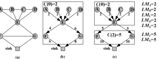
Fig. 2. LM∗for a SP-WSN with seven sensor nodes and a sink. Assume Es = Er = Et = 1 unit, link
capacity is 50 unit, and the maximum feasible energy consumption of all sensor nodes are 20 units. (a) The network topology. (b) the first maximum common rate and corresponding routes (date forwarding directions and rates). (c)LM∗and corresponding optimal routes.
Proof. Firstly, the solution to LPM problem (9),ECxmax, is unique according to Propo-sition 3.3 in Section 3. Therefore, constraints (6), (7), and (11) define the unique feasible region of a rate allocation R = (r1, r2,· · ·, r|V|), say X, which is a convex and compact set (i.e. a polyhedron), since ECxmax is unique. Define a function ϕ(R) = R over X. Ob-viously ϕ(R) is a continuous and increasing function in R. According to Theorem 1 and Proposition 3 in [Radunovic and Boudec 2007], there exists a unique optimal maximin vector(ϕ(r1), ϕ(r2),· · · , ϕ(r|V|)). Therefore, the optimal LM rate allocation LM∗ in our system model is unique.
2.4. Overview of Distributed Solution
Define LMx as the LM rate of a sensor node x∈ V (i.e. LMx is unique, and is an entry of vector LM∗). Let V(r) = {x|LMx ≤ r, x ∈ V} be the set of sensor nodes whose LM rates are not larger than a given real number r. For instance, in Figure 2.41, V(0) = ∅, V(2) ={A,B,C,D,E}, andV(5) ={A,B,C,D,E,F,G}.
Let the sensors inV(r) take their LM rates, and all sensors inV − V(r) take a common rate, DefineC(r) as the maximum feasible common rate of all the sensor nodes inV − V(r):
C(r) = max
<constraints (6),(7), and(11),rz=LMz,∀z∈V(r),rx=ry,∀x,y∈V−V(r))>{ rx}
For instance, in Figure 2.4, C(0) = 2 restricted by bottleneck node E, and C(2) = 5, restricted by bottleneck nodes F and G. Note that bothV(r) and C(r) are functions of r and will be commonly used in our latter discussions.
Current centralized solution [Chen et al. 2007; Hou et al. 2008; Liu et al. 2011] to LM rate allocation can be considered as specific implementations of the max-min programming approach[Radunovic and Boudec 2007]. In our context, max-min programming can compute LM∗by iteratively solving two kinds of LP problems: Maximum Common Rate (MCR) and Maximum Single Rate (MSR). In each MCR-MSR cycle, MCR computesC(r) for all sensor nodes inV − V(r) and then MSR checks whether LMx=C(r) for each nodex∈ V − V(r). The iteration rule ofr for each MCR-MSR cycle is
rn =C(rn−1) r0= 0,
Hence,LM∗ in non-descending order has the following structure:
(C(r0), ..., C(r0), C(r1), ..., C(r1), ..., C(rn), ..., C(rn))
1Note that although Figure 2.4(a) is illustrated as a bidirectional graph for brevity, all the links in it is
[image:7.612.171.445.92.195.2]In Figure 2.4, for instance,LM∗in non-descending order is (2,2,2,2,2,5,5) and it needs two MCR-MSR cycles to computeLM∗ and corresponding optimal routes. It worth noting that although LM∗ is unique, the routes corresponding to LM∗ may not be unique. For instance, fA,B = fB,A = 0 in Figure 2.4(c). However, we can also get a feasible optimal routing corresponding to LM∗, by resetting fA,B = fB,A = 1 and keep all other data forwarding rate constant. However, this route contains a loop.
It can be seen that MCR-MSR approach are not only centralized but also suffer a very large overhead, i.e. solving O(|V|) MCR and O(|V|2) MSR problems. In addition, the routes corresponding to the LM rate allocation computed by above centralized approach may exist loops, which leads to large end-to-end delay and unnecessary network resource costs.
Fig. 3. Logical flow of our distributed DMCR-LMD approach.
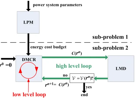
Due to its optimality, our approach, DMCR-LMD iterations, adopts the similar logical flow of max-min programming, but computesLM∗in a fully distributed way and with much lower complexity. Figure 3 shows the logical flow of our distributed approach. After solving LPM locally, nodes run two level of iterations to computeLM∗. The high level is the global DMCR-LMD cycles, and the low level is the iterations of each DMCR.
At each DMCR-LMD cycles, the dual-decomposition based DMCR method calculates the maximum common rate C(r). Then the graph-theoretic scheme LMD determines the LM rates of all nodes inV−V(r) simultaneously rather than solving|V−V(r)|MSR problems one by one. Our LMD scheme requires nearly no calculations and at most 1 control packet per node for thewholeprocedure ofLM∗ calculation. Further more, our distributed approach can guarantee loop-free routes (Lemma 6.2 in Section 6).
3. LOCAL POWER MANAGEMENT
This section focuses on the the first sub-problem (9), the local power management problem, which aims to maximize the average energy consumption ECx for everyx∈ V in a given prediction interval.
3.1. Properties of the LPM problem
Due to our practical power model (e.g. finite battery capacity Bmax, recharging inefficiency, and all possible solar powerhi
x≥0,i∈I), it is difficult to solve LPM problem (9) directly. In addition, not arbitrary given parameters (e.g. Bx1 and Eleak) would result in a feasible solution of the LPM problem, i.e. ECmax
[image:8.612.190.427.215.388.2]battery level and estimated solar power are too small, the final batter level BxL+1 would not be able to reach a largeφeven whenECx= Emin. Consequently, before presenting the algorithm, we first introduce some very important properties of LPM problem and discuss feasible parameter settings in practice.
Proposition 3.1 (Monotonicity). Bxi+1(ECx) is a monotonic non-increasing
func-tion of ECx for any given sloti∈I.
Proof. See the appendix.
Two sufficient conditions to grantee that LPM always has a feasible solution are shown in proposition 3.2.
Proposition 3.2 (Feasibility). Two sufficient conditions to grantee that LPM has a feasible solution are
∀i∈I, hix−Emin≥Eleak/η (12)
Bx1+η∑ i∈I
(hix−Emin)−EleakL≥φ (13)
Proof. See the Appendix.
In practice, condition (12) and (13) nearly always holds for daytime of sunny days with carefully selected final state parameterφ. We test this based on a solar powered sensor node with a 9×3.8cm2 solar panel. For night or bad-weather days, neither constraints (12) nor (13) would be guaranteed. However, (12) and (13) are sufficient conditions for feasibility of LPM problem but not necessary conditions to ensure ENO (i.e. battery is not depleted for every slot). We can set φ carefully to store energy during daytime to avoid battery exhausting during night.
Finally, the optimal solutionECmax
x has the following property.
Proposition 3.3 (Optimality and Uniqueness). If there exist two energy consump-tion levels ECx1 and ECx2 ∈ [Emin, Emax]. ECx1 is the maximal ECx that satisfies Bi+1
x (ECx)≥0, ∀i∈I, and ECx2 is the maximal ECx that satisfies the BiL+1(ECx) =φ.
The optimal solution of sub-problem (9) isECxmax= max(Emin,min(ECx1, ECx2,Emax)).
Proof. From proposition 3.1, ECxmax = min(ECx1, ECx2) can satisfy both the con-straints (4) and (5). ConsiderECx∈[Emin,Emax], Proposition 3.3 obviously holds.
3.2. LPM Algorithm
Based on the properties 3.1 and 3.3, we design the LMP algorithm. The pseudo-code is shown in Algorithm 1.
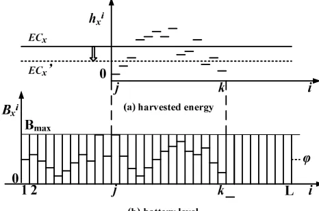
The main idea of the LPM algorithm is to gradually decease ECx from a theoretical upper bound (line 1) until both the two constraints ∀i∈ I, Bi+1
x ≥ 0 and BxL+1 ≥φ are just guaranteed. The slot pointer i represents the current slot and j records slot 1 or the last slot in which the battery level reaches Bmax.L1 andL2 represent the number of slots betweenj and i, in whichECx is smaller than and larger than the harvested solar energy respectively. For instance, Figure 4.a shows the value of aECx and solar energy from slot j to a slotk (Bk+1
x <0) and Figure 4.b shows the corresponding battery level in all slots beforek+ 1. In Figure 4, ifi=k, thenL1= 6, L2= 8.E represents
E=Bxj+ ∑
ECx≥ht x
htx+ ∑
ECx<ht x
ALGORITHM 1:The operation of a nodex∈ Vat the beginning of each prediction interval (LPM algorithm).
Input:Initial battery levelB1
x, battery capacity Bmax, final state constraint parameterφ, recharging efficiency
η, leakage Eleak, and harvesting profilehix,∀i∈I.
Output:The maximum feasible energy consumptionECmax
x 1: ECx←min(Emax,
∑
i∈I(h i x+B
1
x−φ)/L−Eleak); 2: i←1;j←1;Bxj←Bx1;L1←0;L2←0;E←Bx1;
3: whilei≤Ldo
4: if hix> ECxthen /∗recharging in sloti∗/ 5: Bi+1
x =Bix+η(hix−ECx)−Eleak; 6: L1←L1+ 1;
7: E←E+ηhi
x−Eleak;
8: else /∗discharging in sloti∗/ 9: Bi+1
x =Bix+hix−ECx−Eleak; 10: L2←L2+ 1;
11: E←E+hi
x−Eleak;
12: end if
13: if Bi+1
x >Bmaxthen/∗battery is overcharged∗/ 14: Bi+1x ←Bmax;
15: E←Bmax; 16: j←i+ 1; 17: Bj
x←Bmax; 18: L1←0;L2←0; 19: i←i+ 1;
20: else if Bxi+1<0then /∗decreaseECx∗/
21: ECx←E/(ηL1+L2); 22: i←j;
23: Bi
x←Bjx;E←Bxj;L1←0;L2 ←0;
24: else if Bxi+1< φ∧i=Lthen/∗decreaseECx∗/
25: ECx←(E−φ)/(ηL1+L2); 26: i←j;
27: Bi
x←Bjx;E←Bxj;L1←0;L2 ←0; 28: else
29: i←i+ 1;
30: end if
31:end while
32:returnmax(ECx,Emin)
With aECx, there may be a slot when the battery level reaches Bmax(line 13).j always records such latest slot.L1,L2, andEare updated to record the corresponding values after slot j.ECx is only updated by lines 21 and 25.
Lemma 3.4. Let ECx′ be the updated ECx, thusEC
′
x must be smaller thanECx.
Proof. For line 21, sinceBxk+1(ECx)<0, we have
ECx > (Bjx+
∑
ECx>ht x
htx+ ∑
ECx<ht x
ηhtx−(L1+L2)Eleak)/(ηL1+L2)
For line 25, similarly, we can obtainBL+1
x < φ⇔EC
′
x< ECx.
SinceECxis feasible for all slots beforek+ 1,EC
′
xis therefore feasible for all slots before k+ 1, according to Proposition 3.1 and Lemma 3.4. Consequently, having calculatedECx′, the LPM algorithm only rechecks the feasibility ofECx′ in slotk+ 1. To this end, the LPM algorithm recalculates the battery levels from slotj to slotk+ 1 (lines 22 and 26), because Bjxremains Bmax orBx1for anyEC
′
x< ECx, according to Proposition 3.1.
For a calculatedECx′, let the corresponding numbers of slots betweenj andkbeL′1and L′2 respectively, in which harvesting energy is smaller and larger thanECx′. For instance, in Figure 4,L′1=L1+ 4 andL
′
2=L2−4. When the energy consumption level drops from ECxto EC
′
x, the following three cases would happen.
Fig. 4. An example to explain LPM algorithm.
Lemma 3.5. For any given 1 < k ≤ L such that Bxk+1(ECx) < 0 if k < L; or Bk+1
x (ECx) < φ, otherwise the last updated ECx is the maximum feasible energy
con-sumption for all slots beforek.
Proof. See the Appendix.
Theorem 3.6. The output of the LPM algorithm is the optimal solution of sub-problem (9).
Proof. According to Lemma 3.5, the last updatedECxis always the maximum feasible energy consumption for all slots before k+ 1, and the algorithm ends when k = L and Bkx+1(ECx)≥φ.
Now we discuss the computation overhead of the LPM algorithm. For a given j and k, both the cases 2 and 3 happen at mostk−j+ 1 times beforek is updated (because there are k−j+ 1 slots between slots k and j). Consequently, in above two worst cases, our LPM needs at most O(L2) simple arithmetic calculations to compute ECmax
[image:11.612.185.418.252.406.2]4. DISTRIBUTED MCR
Let the maximum common rate computed in the last DMCR-LMD cycle ber≥0, then the current DMCR aims to computeC(r) for all nodes inV − V(r) (please see Figure 3 for the logical flow of our DMCR-LMD approach). For instance, if the current DMCR is in the first DMCR-LMD cycle, then r= 0. C(r) can be calculated by solving the following problem: ∀x, y∈ V − V(r), z∈Nx, p∈ V(r)
Maximize ∑
x∈V−V(r)
rx (14)
Subject to r
x−ry= 0 (15)
rx−r≥0 (16)
rp−LMp= 0 (17)
0≤fx,y ≤cx,y (18)
rx+
∑
z∈Nx fz,x−
∑
z∈Nx
fx,z= 0 (19)
ECxmax−Esrx−Er
∑
z∈Nx
fz,x−Et
∑
z∈Nx
fx,z ≥0 (20)
Constraint (15) enforces allrxto be equal, according to the objective of the MCR problem. Constraints (19) and (20) refer to flow conservation law and energy constraints respectively. Also, sincex∈ V − V(r), constraint (16) ensures that the lower bound ofrx isr. Further, constraint (17) highlights that every nodep∈ V(r) should keep their sensing rate as LMp which has been determined by previous DMCR-LMD cycles.
The objective of problem (14) is to calculate the maximum common rateC(r) of sensor nodes inV−V(r) (i.e.rx, x∈ V−V(r)), as well as the corresponding optimal routes (fx,z, z∈ Nx). DMCR is based on dual-decomposition which is commonly used in distributed network optimization. In contrast to existing approaches, however, DMCR deals with two novel problems as follows:
Heterogeneous Decomposition. From the problem formalization (14)-(20) we can see
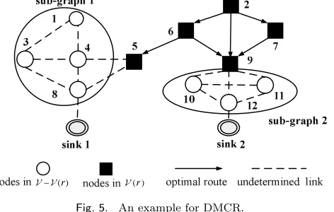
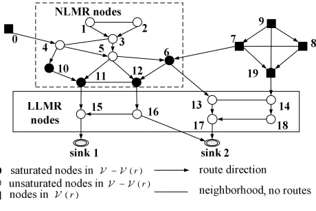
that not only all sensor nodes inVbut also every nodex∈ V − V(r) and every nodez∈Nx are part of the current DMCR calculation. A simple example is shown in Figure 5, nodes 2, 6, and 7 who are inV(r), will not involve in current DMCR, because their LM rates and the corresponding optimal routes (represented as directional solid lines) have been determined in previous DMCR-LMD cycles. Since the current DMCR calculation is to compute the maximum common rateC(r) of the nodes inV − V(r) (i.e. nodes 1, 3, 4, 8, 10, 11, and 12), as well as the routes (flows over links that represented as dotted lines), not only the nodes inV − V(r), but also the nodes 5 and 9 who are the neighbors of nodes 4, 8, 10, 11 are part of the current DMCR calculation. Nodes 5 and 9 only calculate the optimal flows over links (5, 4), (5, 8), (9, 10), and (9, 11). Our DMCR manages to decouple the original problem (14) into different subproblems for each nodex∈ V − V(r) and each nodez∈Nx.
Disconnected Network Topology.Current dual-decomposition-based schemes always
calculation, which may result in less DLMD cycles than that of centralized MCR-MSR. Our simulation results show that the number of DMCR-LDM cycles can be 150% less than that of MCR-MSR cycles, which will significantly reduce the system convergence time and overheads.
( )r
−
V V V( )r
Fig. 5. An example for DMCR.
We construct the dual problem of the primary problem (14) by introducing the Lagrange multipliers λx, νx for energy constraint (20) and flow conservation constraint (19) respec-tively at each nodez∈Nx, x∈ V − V(r), and the Lagrange multiplierρx,y for rate equality constraint (15) for node pairs x∈ V − V(r) andy ∈(V − V(r))∩Nx. The corresponding Lagrangian is
L(r, f, λ, υ, ρ)
= ∑
x∈V−V(r)
rx(1−λxEs−υx+
∑
y∈Nx∩(V−V(r))
(ρx,y−ρy,x))
+ ∑
x∈V−V(r)
∑
z∈Nx
(fx,z(υz−υx−Etλx−Erλz))
+ ∑
x∈V−V(r)
λxECxmax (21)
The dual function is:
D(λ, ν, ρ) = sup r≤rx,0≤fx,z≤cx,z
L(r, f, λ, υ, ρ) (22)
Then we have the dual problem
Minimize D(λ, ν, ρ) (23)
Subject to λ≥0 (24)
Since the objective function of problem (14) is not strictly concave (i.e. linear) in both primary variables r and f, the solution should be recovered [Xiao et al. 2004]. We use the strictly concave term ∑x∈V−V(r)logrx to replace the objective function(14), because maximizing rx is equal to maximizing log(rx) with the equal constraint (15). We also add a small strictly concave regularization term−ε∑x∈V−V(r)∑z∈Nxf2
x,zfor variablef to the objective function (4). The regularized objective of the primary problem (14) is
∑
x∈V−V(r)
logrx−ε
∑
x∈V−V(r)
∑
z∈Nx
[image:13.612.193.429.135.285.2]By choosingεsmall enough, the solution of the regulated problem can be arbitrary close to that of the original problem (14). The corresponding regularized dual problem is
Minimize sup
rx≥r,0≤fx,z≤cx,z
∑
x∈V−V(r)
logrx−rx(λxEs+υx−
∑
y∈Nx∩(V−V(r))
(ρx,y−ρy,x))
+ ∑
x∈V−V(r)
∑
z∈Nx
(fx,z(υz−υx−Etλx−Etλz)−εfx,z2 ) +
∑
x∈V−V(r)
λxECxmax
Subject to λ≥0
(26)
We use a sub-gradient algorithm to solve the regulated dual problem (26). The algorithm starts from the initial values λ(0)x ,ν
(0) x ,ρ
(0)
x,y: For the kth iteration step of the sub-gradient algorithm, each nodexinV − V(r) solves the following two simple maximizing problems:
rx(k)= arg max
r≤rx(logrx−rx(υ (k) x +
∑
y∈(Nx∩V−V(r))
(ρ(xyk)−ρyx(k))−λ(xk)Es) (27)
fx,z(k)= arg max
z∈Nx,cx,z≥fx,z≥0(fx,z(υ (k) z −υ
(k) x −Etλ
(k) x −Erλ
(k) z )−εf
2
x,z) (28)
For each node x∈ V − V(r), the next stepλ(xk+1),υ (k+1) x ,ρ
(k+1)
x,y , y∈Nx∩(V − V(r))are computed as
λ(xk+1)=|λ(xk)−l(k)(ECxmax−Esr (k) x −Er
∑
z∈Nx
fz,x(k)−Et
∑
z∈Nx
fx,z(k))|+ (29)
υx(k+1)=υx(k)−l(k)
( ∑
z∈Nx
(fx,z(k)−fz,x(k))−rx(k)
)
(30)
ρ(x,yk+1)=ρ(x,yk)−l(k)
(
ry(k)−r(xk)
)
(31)
Wherel(k)is the step length of thekthiteration, one condition for the convergence of the subgradient algorithm is (see Lemma 6.1 in Section 6.1):
∞ ∑
k=1
(l(k))2→0,
∞ ∑
k=1
l(k)→ ∞ (32)
For instance we can set L(k)= 1/k. From (27)-(31), each nodex∈ V − V(r) exchanges all updated flow and dual variables with its neighbors in V − V(r), but only obtain fz,x,λz, andνz from its neighborsz∈ V(r)∩Nxin every iteration step.
As we have mentioned, besides every node x∈ V − V(r), every node z ∈ V(r)∩Nx is part of the current DMCR calculation to compute the the amount of data forwarded over links (z, x) should also be determined. The calculation is based on the following Theorem:
Theorem 4.1. For each node z∈ V(r)∩Nx, x∈ V − V(r), its optimal incoming flows
are sent by nodes only p∈Nz∩ V(r)and have been determined before the current DMCR
calculation.
Proof. According to Lemma 6.3 in Section 6.2, sincez∈ V(r), for any forwarding path P(p, z), p∈ V(r). Sincepisz,sneighbor,p∈N
According to Theorem 4.1, the forwarding ratefz,p, p∈Nz∩ V(r) have been predeter-mined in previous DMCR-LMD cycles. Sincerzhas also be determined (i.e.LMz), nodez only updatesfz,x,x∈ V − V(r) in itskthstep as follows
fz,x(k)= arg max
cz,x≥fz,x≥0,z∈Nx∩V(r),x∈V−V(r)
(fz,x(υx(k)υ (k) z −Etλ
(k) z −Erλ
(k) x )−εf
2
z,x) (33)
Then, theλ(zk+1) andυ (k+1)
z are updated as
λ(zk+1)=|λ(zk)−l(k)(ECzmax−EsLMz
−Er
∑
p∈Nz∩V(r)
fp,z−Et
∑
x∈Nz∩(V−V(r))
fz,x(k))|+ (34)
υ(zk+1)=υz(k)−l(k)
∑
x∈Nz fz,x(k)−
∑
p∈Nz∩V(r)
fp,z−LMz
(35)
In summary, every nodex∈ V − V(r) updates its primary and dual variables using (27)-(31), and every nodez∈ V(r)∩Nx, x∈ V − V(r) in updates its primary and dual variables (33)-(35). It is obvious that all information for (27)-(35) is either local or can be obtained by neighbor nodes, therefore DMCR is fully distributed.
DMCR calculates C(r) (i.e. maximized rx) and corresponding optimal routes (i.e. fx,y and fy,x, x ∈ V − V(r), y ∈ Nx). One nice property of our approach is that the optimal routes calculated by DMCR is loop-free( Lemma 6.2 in Section 6).
In order to focus on the global multi-objective LM rate allocation problem, DMCR only adopts the basic dual-decomposition techniques: augmented Lagrangian and sub-gradient algorithms, which may result in relatively large convergence time. However, the convergence speed of DMCR could be significantly improved (e.g. hundreds of times faster) by using recent-proposed distributed convex optimization techniques such as [Necoara and Suykens 2008; Wan and Lemmon 2009].
When current DMCR computation completes, every nodex∈ V − V(r) recordsC(r) and data forwarding rates over its optimal incoming and outgoing links, for the forthcoming LMD to determine whether C(r) is its LM rate or not (please see Figure 3 for the logical flow of our DMCR-LMD approach).
5. LM RATE DETERMINATION
Let C(r) be the maximum common rate computed by the last DMCR. After computing C(r), each nodex∈ V − V(r) should determine whetherC(r) is its LM rate (i.e.LMx) or not (Please refer to Figure 3 for the logical flow of our DMCR-LMD approach.). This can be achieved by solving the following LP problem (i.e. the MSR problem)
Maximize rx (36)
Subject to ry=C(r),∀y∈ V − V(r)− {x} (37)
constraints (16)−(20)
For readability, we call sensor nodes inV − V(r) whose LM rates are equal to and larger thanC(r) as New LM Rate (NLMR) nodes and Larger LM Rate (LLMR) nodes respectively. Obviously, the goal of solving|V − V(r)|LP problems (36) is to determine all NLMR nodes and LLMR nodes. In this section, we develop LMD, a fully distributed graph-theoretic scheme to achieve this goal. In contrast to solve|V − V(r)|LP problems one by one, LMD manages to determine the state of each nodex∈ V −V(r) simultaneously (i.e.xis a NLMR node or LLMR node), with extremely low overhead.
5.1. Graph-theoretic Understanding of the LM rate Determination Problem
Before presenting the LMD scheme, we first analyze the LM rate determination problem from graph theory perspective. We define a temporary graph formed after the last DMCR:
Definition5.1 (Temporary Graph). A temporary graph G(S ∪ V,F, r) forms after the calculation of the last C(r), where F is the set of allocated forwarding rate over every link (i.e. end-to-end routes from network-wide perspective), which is calculated by the last DMCR and previous DMCR-LMD cycles.
( )r
V
( )r
−
V V
( )r
−
V V
Fig. 6. An example of a temporary graph.
Figure 6 illustrates an example of a temporary graph2. Actually, the process of theLM∗ calculation can be seen as determining the new LM rates and corresponding temporary graphs step by step. The first temporary graph forms after the calculation ofC(0), and the last temporary graph forms when all LM rates have been found and represents the optimal routing corresponding toLM∗.
Definition5.2 (Saturated Node and Unsaturated Node). We call a sensor node x in a temporary graphG(S ∪ V,F, r) a saturated node, if
Esrx+ Er
∑
y∈Nx
fy,x+ Et
∑
y∈Nx
fx,y−ECxmax= 0
or
fx,y =cx,y,∀y∈Nx
; otherwise,xis called an unsaturated node.
2It worth noting that Figure 6 is a temporary graph, but Figure 5 is not a temporary graph, because Figure
[image:16.612.195.425.285.439.2]Definition5.3 (Path and Forwarding Path). Given a temporary graph G(S ∪ V,F, r), a path P(s, d) with source s and destination d, s ∈ V, d∈ S ∪ V, is a sequence of links. If fx,y >0,∀(x, y)∈P(s, d), thenP(s, d) is a forwarding path. IfP(s, d) is a forwarding path, it is called the source node s′s downstream path, and the destination noded′s upstream path. If all sensor nodes in a path is unsaturated, then we call this path an unsaturated path, otherwise we call it a saturated path.
An arbitrary path may not be a forwarding path, but each sensor nodex∈ V must have a downstream forwarding path to the sink in every temporary graphG(S ∪V,F, r),r≥C(0), because xmust have a non-zero sensing rate (i.e.rx≥C(0)>0) for any temporary graph, and the flow injected into the network (i.e. rx) must be transmitted to the sink, according to the flow conservation law.
Theorem 6.8 in Section 6.2 provides a condition to determine the state (NLMR or LLMR) of a node in V − V(r): Let P(x, s) ∈ G(S ∪ V,F, r) be an arbitrary path from a node x∈ V − V(r) to an arbitrary sinks∈ S. Except for the destinations, this path consists of nodes only inV −V(r). If all such paths are unsaturated, thenxis a LLMR node. Otherwise, xis a NLMR node.
From theorem 6.8, saturated nodes inV −V(r) form a saturated cut or multiple saturated cuts between a set of unsaturated nodes inV−V(r) and all sinks in a given temporary graph. Take Figure 6 for instance, saturated nodes 10, 11, 12, and 6 form a cut which separates the set of unsaturated nodes 1, 2, 3, 4, and 5 from the two sinks. All possible forwarding paths from these nodes to the two sinks, which only consists of nodes inV − V(r), must via the saturated nodes 6, 10, 11, and 12. According to Theorem 6.8, nodes 1 2, 3, 5, 6, 10, 11 and 12 are NLMR nodes and other unsaturated nodes inV − V(r) are LLMR nodes.
5.2. The LMD scheme
Fig. 7. Illustration of LMD operating durations.
The Pseudo-code of the LMD scheme is described in Algorithm 2. The LMD scheme multicasts a one-hop control packet, Max-min Notice (MN) packet. As shown in Figure 7, LMD starts at timeT0(r) when the last DMCR is finished, and complete at timeTn(r) when next DMCR starts. The upper bound of the duration[T0(r), Tn(r)] is determined by the per-hop transmission delay and network diameter (see the proof of Lemma 6.14 in Section 6.2), which can be easily estimated in practice.
AtT0(r), every nodexinV − V(r) recordsC(r) and it local flow information calculated by the last DMCR. Consequently, x can locally determine its state (i.e. saturated or un-saturated). At T0(r), every node initiates as a LLMR node (line 1, in self check at T0(r)), it then checks whether it is a saturated node or not (line 3) by simply calculating its local constraint (20). After self-checking, every saturated sensor nodexinV − V(r) sets its state as NLMR and multicasts a one-hop MN packet to all its upstream neighbors inV − V(r) (lines 3-7). During the MN packet transmission phase, the MN packets generated by the saturated nodes inV − V(r) are relayed through their upstream neighbors inV − V(r).
[image:17.612.147.464.388.453.2]its state as NLMR (line 2), then it records the ID of the sender of this packet (line 3). Then xchecks whether its every downstream neighbor inDx(r) has sent it a MN packet and its upstream neighbor setUx(r) is non-empty (line 4). If yes,xmulticasts a MN packet to all node(s) inUx(r) (line 5).
ALGORITHM 2:Pseudo-code of the LMD for a sensor nodex∈ V − V(r).
Control Packets:
Maxmin Notice(MN)
Variables:
x.state: this value could be NLMR or LLMR, determine this value is the objective of LMD.
Nx(r) =Nx∩(V − V(r)).
Dx(r) ={y|y∈Nx(r), fx,y>0}: the set ofx’s all downstream neighbors in setNx(r).
Ux(r) ={y|y∈Nx(r), fy,x>0}: the set ofx’s all upstream neighbors in setNx(r).
SNx: the set of neighbors who have sent MN packets tox.
Function:
multicast(Ux(r)): multicast a MN packet to all nodes in the setUx(r).
Self Check at T0(r)
1:x.state←LLMR;
2:SNx←∅;
3:if xis saturatedthen
4: x.state←NLMR; 5: if Ux(r)̸=∅then
6: multicast(Ux(r));
7: end if
8:end if
Receive a MN packet from y∈Dx(r) before Tn(r) 1:if xis unsaturatedthen
2: x.state←NLMR; 3: SNx←SNx∪ {y};
4: if(Dx(r) =SNx)∧(Ux(r)̸=∅)then
5: multicast(Ux(r));
6: end if
7:end if
Take Figure 6 for example, nodes 6, 10, 11, and 12 know that they are saturated after self-checking and send MN packets to their upstream neighbors 4 and 5 respectively. At Tn(r), the unsaturated nodes 1, 2, 3, 4, and 5 have received MN packets but only nodes 3 and 5 have been sent a MN packet respectively. The MN packet transmission procedure is: firstly 10→4 and{11, 12, 6} →5, then 5→ {3, 4}, finally 3→ {1, 2}.
Consequently, every nodex∈ V −V(r) manages to determine its state (LLMR or NLMR) at Tn(r) as follows: xis a NLMR node, if it is a saturated node, or an unsaturated node and has received a MN packet; xis a LLMR node, ifxis an unsaturated node and has not receive any MN packet.
6. PERFORMANCE ANALYSIS
In this section, we provide rigorous analysis of the system performance. The main results are as follows.
Firstly, DMCR converges arbitrarily close to the optimal solution of problem (14) (Lemma 6.1). The routes computed by any DMCR is loop-free, including the optimal routes with regards toLM∗ (Lemma 6.2).
Secondly, LMD let each node inV − V(r) know it is a NLMR node or LLMR node before Tn(r) (Theorem 6.16). LMD determines the LM rate for every node with at most 1 control packet for the whole procedure ofLM∗ calculation (Theorem 6.17).
Thirdly, the whole system (LPM, DMCR, and LMD) converges to optimal LM rate allocationLM∗ and corresponding optimal routes (Theorem 6.18).
6.1. Analysis of DMCR
Lemma 6.1. Each DMCR can converges arbitrarily close to the optimal solution of prob-lem (14) asε→0.
Proof. Let the optimal dual variables be (λ, ν, ρ)∗ that minimize the regulated dual functionDε(λ, ν, ρ) (26). At thekth step of the subgradient algorithm, we have
∥(λ, ν, ρ)(k+1)−(λ, ν, ρ)∗∥22
=∥(λ, ν, ρ)(k)−l(k)g(k)−(λ, ν, ρ)∗∥22
=∥(λ, ν, ρ)(k)−(λ, ν, ρ)∗∥22−2l(k)g(k)T((λ, ν, ρ)(k)−(λ, ν, ρ)∗) + (l(k))2∥g(k)∥22 ≤ ∥(λ, ν, ρ)(k)−(λ, ν, ρ)∗∥22−2l(k)(Dε((λ, ν, ρ)(k))−D∗ε((λ, ν, ρ)∗)) + (l
(k))2∥g(k)∥2 2
where∥ · ∥is the Euclidean norm operator and the last inequality is based on the definition of subgradient. Applying the inequality above recursively, we have
∥(λ, ν, ρ)(1)−(λ, ν, ρ)∗∥22−2 k
∑
i=1
l(i)(Dε((λ, ν, ρ)(i))−D∗ε((λ, ν, ρ)∗)) + k
∑
i=1
(l(i))2∥g(i)∥22
≥ ∥(λ, ν, ρ)(k+1)−(λ, ν, ρ)∗∥22≥0 Assume the subgradient is bounded ∥g(k)∥2
2 ≤ G (this can be easily achieved by adding sufficient large upper bounds for bothr andf), then we have
Dε((λ, ν, ρ)(k))−Dε∗((λ, ν, ρ)∗)≤ ∥(λ, ν, ρ)
(1)−(λ, ν, ρ)∗∥2 2+G2
∑k i=1(l
(i))2
2∑ki=1l(i)
According to step size updating rule (32), i.e.∑∞i=1(l(k))2→0, ∑∞ i=1l
(i)→ ∞, we have
lim
k→∞Dε((λ, ν, ρ)
(k)) =D∗
ε((λ, ν, ρ)∗)
Consider the strong duality of the system and the expression of Dε(·), we can conclude that asε→0, DMCR converges to the optimal solution of problem (14).
Lemma 6.2. The routes calculated by any DMCR are loop-free.
Proof. Letλ∗x, νx∗, fx,y∗ be the optimal value ofλx, νx, fx,y respectively. From equations (18) and (23), we have:
fx,z∗ =
{
−(∆υ∗+Etλ∗x+Erλ∗z) 2ε
−(∆υ∗+Etλ∗x+Erλ∗z) 2ε >0 0 −(∆υ∗+Etλ∗x+Erλ∗z)
Where ∆νx∗=νx∗−νz∗. Suppose there is a loop such thatfx∗1,x2>0, fx∗2,x3>0,· · ·, fxn,x∗ 1> 0, which implies:
υx∗1−νx∗2<−Etλ∗x1−Erλ∗x2
· · ·
υ∗xn−νx∗1<−Etλ∗xn−Erλ∗x1
Taking a telescopic sum of above inequations from 1 ton, we get:
0<−(Et+ Er) n
∑
i=1 λ∗xi
Which is impossible, because (Et+ Er)
∑n
i=1λ∗xi is always non-negative.
6.2. Analysis of LMD
Lemma 6.3. Consider an arbitrary forwarding pathP(x, y)in a temporary graph G(S ∪ V,F, r), if y∈ V(r), thenx∈ V(r).
Proof. We prove Lemma 6.3 by contradiction. Suppose there is a forwarding path
P(x, y), x∈ V − V(r) and y∈ V(r), then we haveLMx≥C(r)> LMy. Therefore, we can setrx=C(r)−∆randry =LMy+ ∆r, where ∆r <(LMy+LMx)/2, by reducing the ∆r amount of flow overP(x, y). Since the amount of flow overP(x, y) is reduced, the unchanged sensing rates of other nodes onP(x, y) are still feasible. As a result, we have a new feasible rate allocation, in whichrx=C(r)−∆r, ry=LMy+ ∆r, rm=C(r),∀m∈ V − V(r)− {x}, and rn = LMn,∀n ∈ V(r)− {y}. This new rate assignment is lexicographically greater thanLM∗, which conflicts with the fact thatLM∗ is the unique lexicographically optimal feasible rate allocation (Theorem 2.3).
Lemma 6.3 means that data traffic generated by any node in V − V(r) will not pass any node inV(r).
Definition 6.4. Real and Fake saturated nodes: Consider a saturated node x, and an unsaturated node y, x, y ∈ V − V(r). If there exist two forwarding paths P(y, x) and P(y, s) s ∈ S in G(S ∪ V,F, r), where P(y, s) consists of pure unsaturated nodes, then xis called a fake saturated node. Otherwise, it is a real saturated node.
Lemma 6.5. For a temporary graphG(S ∪ V,F, r), the probability that a fake saturated node exists is zero.
Proof. Suppose there is a fake saturated nodexin a temporary graph inG(S+V,F, r), such that an unsaturated nodeyhas a forwarding path toxand a forwarding path to a sink. In this case, xcan also be unsaturated by reducing the ∆ramount of flow on P(y, x) and increasing the same amount of flow onP(y, s). All nodes inV−V(r) can still keep the sensing rate ofC(r). As long as ∆ris smaller than the residual capacity of pathP(y, s), this is still a feasible solution to DMCR. Hence, nodexis not the bottleneck of the network. Letλ∗xbe the optimal dual variable λx computed by any DMCR. According to complementary slackness condition [Boyd and Vandenberghe 2004],λx>0, ifxis saturated;λx= 0, otherwise. Since λxis a continuous variable, there exists infiniteλx>0 but only oneλx= 0. Therefore, the probability thatxis a fake saturated node is zero.
For instance, the probability that node 15 in Figure 6 is a saturated node is zero.
Lemma 6.6. For a temporary graphG(S ∪ V,F, r), all real saturated nodes inV − V(r)
Proof. Supposed a real saturated node isxis a LLMR node, then we can writerx= ∆r+C(r), where ∆r >0 and all other nodes in V − V(r) keep the sensing rate ofC(r). To guarantee feasibility, xhas to reduce its ∆rrelay flow of its upstream nodes. Lety be an arbitrary upstream node ofx, thenyhas to reduce the flow onP(y, x) and increase the same amount of flow on a forwarding pathP(y, s), according to the flow conservation law. To relay the additional flow,P(y, s) must consist of all unsaturated nodes, which meansx is a fake saturated node. This conflicts with the supposition.
Lemma 6.7. For a forwarding path P(x, y) in G(S ∪ V, F, r), x, y ∈ V − V(r). If x is unsaturated and y is saturated, then there must exist at least one saturated node on every path P(x, s),∀s∈ S.
Proof. According to Lemmas 6.5 and 6.6, lemma 6.7 obviously holds.
Since there is no fake saturated node, in later discussions we will directly use the term ”saturated node” as a shorthand notion of ”real saturated nodes”.
Theorem 6.8. LetP(x, s)∈ G(S∪V,F, r)be an arbitrary path from a nodex∈ V−V(r) to an arbitrary sink s ∈ S. Except for the destination s, this path consists of nodes only in V − V(r). If all such paths are unsaturated, then xis a LLMR node. Otherwise, x is a NLMR node.
Proof. Ifxis a saturated node, then it is a NLMR node according to lemma 6.6. Ifxis an unsaturated node, supposexis a LLMR node, then we can writerx= ∆r+C(r), and ry =C(r) and rz =LMz, where ∆r > 0, y ∈ V − V(r), and z ∈ V(r). According to flow conservation law, there must exist a forwarding path P(x, s),s∈ S, which is able to relay the incremental flow ∆r, i.e.P(x, s) must consist of pure unsaturated sensor nodes and the minimal residual capacity of node onP(x, s) is larger than ∆r, which conflict with the supposition.
Definition6.9 (Temporary Upstream Path Enclosure (TUPE)). For a given G(S ∪ V,F, r). Let P(x) be the union of unsaturated nodes in V − V(r) on all upstream paths of an arbitrary saturated nodex∈ V − V(r). Denote the saturated cut X be a set of sat-urated node in V − V(r) such that ∀x, y ∈ X,P(x)∩ P(y) ̸= ∅. We define a TUPE as
P(X) =∪x∈XP(x).
It can be seen all nodes in P(X) are unsaturated in V − V(r) and X separates these unsaturated nodes from all sinks. For example, in Figure 6,X ={6,10,11,12}andP(X) = {1,2,3,4,5}.
Lemma 6.10. All unsaturated nodes in a TUPEP(X)are NLMR nodes.
Proof. Since every unsaturated sensor node y in a TUPE must has one downstream saturated node, there must be a saturated node ony,s all downstream paths, according to Lemma 6.7. Furthermore, according to theorem 6.8, yis a NLMR node.
Definition 6.11. For a node y ∈ P(X), let P(y, X) be set of all forwarding paths P(y, x), x∈X. DenoteD(y, X) as the maximal hop count of all forwarding paths inP(y, X). In addition, denoteDis(y, X) = 0, ify∈X.
For example, in Figure 6, X = {6,10,11,12}, D(5, X) = 1, D(4, X) = 2, and Dis(10, X) = 0.
Lemma 6.12. For any node y∈P(X), Dis(y, X)≤ |P(X)|.