This is a repository copy of
Data-driven Control Design Schemes in Active Distribution
Grids: Capabilities and Challenges
.
White Rose Research Online URL for this paper:
http://eprints.whiterose.ac.uk/146460/
Version: Accepted Version
Proceedings Paper:
Karagiannopoulos, S, Dobbe, R, Aristidou, P orcid.org/0000-0003-4429-0225 et al. (2
more authors) (2019) Data-driven Control Design Schemes in Active Distribution Grids:
Capabilities and Challenges. In: Proceedings of the 2019 IEEE PowerTech conference.
2019 IEEE Milan PowerTech, 23-27 Jun 2019, Milan, Italy. IEEE . ISBN 9781538647226
https://doi.org/10.1109/PTC.2019.8810586
This conference paper is protected by copyright. Uploaded in accordance with the
publisher's self-archiving policy.
[email protected] https://eprints.whiterose.ac.uk/
Reuse
Items deposited in White Rose Research Online are protected by copyright, with all rights reserved unless indicated otherwise. They may be downloaded and/or printed for private study, or other acts as permitted by national copyright laws. The publisher or other rights holders may allow further reproduction and re-use of the full text version. This is indicated by the licence information on the White Rose Research Online record for the item.
Takedown
If you consider content in White Rose Research Online to be in breach of UK law, please notify us by
Data-driven Control Design Schemes in Active
Distribution Grids: Capabilities and Challenges
Stavros Karagiannopoulos
∗‡, Roel Dobbe
‡, Petros Aristidou
§, Duncan Callaway
‡, Gabriela Hug
∗ ∗ EEH - Power Systems Laboratory, ETH Zurich, Physikstrasse 3, 8092 Zurich, Switzerland ‡ Department of Electrical Engineering & Computer Sciences, UC Berkeley, Berkeley, USA §School of Electronic and Electrical Engineering, University of Leeds, Leeds LS2 9JT, UKEmails:{karagiannopoulos, hug}@eeh.ee.ethz.ch,{dobbe, dcal}@berkeley.edu, [email protected]
Abstract—Today, system operators rely on local control of distributed energy resources (DERs), such as photovoltaic units, wind turbines and batteries, to increase operational flexibility. These schemes offer a communication-free, robust, cheap, but rather sub-optimal solution and do not fully exploit the DER capabilities. The operational flexibility of active distribution net-works can be greatly enhanced by the optimal control of DERs. However, it usually requires remote monitoring and communi-cation infrastructure, which current distribution networks lack due to the high cost and complexity. In this paper, we investigate data-driven control algorithms that use historical data, advanced off-line optimization techniques, and machine learning methods, to design local controls that emulate the optimal behavior without the use of any communication. We elaborate on the suitability of various schemes based on different local features, we investigate safety challenges arising from data-driven control schemes, and we show the performance of the optimized local controls on a three-phase, unbalanced, low-voltage, distribution network.
Index Terms—optimal control, data-driven control design, active distribution networks, OPF, machine learning
I. INTRODUCTION
Distribution systems are undergoing a tremendous transfor-mation due to the introduction of large shares of Distributed Generators (DGs), mainly renewables. Although DGs bring some uncertainties in distribution grids, they can provide significant operational flexibility, amplifying the role of Distri-bution Networks (DNs) [1]. Their ability is further enhanced when combined with other Distributed Energy Resources (DERs), such as batteries and flexible loads.
The control of DERs is vital to ensure a secure, reliable and cost-effective DN operation. A first option is centralized schemes that require monitoring and communication infras-tructure and usually rely on optimization methods. These schemes have become popular due to theoretical develop-ments in the nonlinear AC power flow [2] and advances in computational power that allow for the real-time solution of such problems. Several researchers have proposed system-wide optimal operation methods by coordinated control of DERs, e.g. [3], [4]. Another option is local control schemes, e.g. [5], that rely only on local information to modify the DER behavior. They are simple, robust, communication-free and are already embedded in several grid codes. However, these methods usually employ a one-size-fits-all approach, where the same control parameters are employed in all DNs and types of DERs. Finally, distributed approaches, e.g. [6], use limited
communication between different DERs to coordinate them and achieve a close-to-optimal operation.
In this paper, we investigate data-driven control design methods that have gained a lot of attention lately. Such meth-ods are hybrid as the controllers are ”trained” using offline centralized approaches, but the derived local controls can be used when no communication infrastructure is available [7], [7]–[12]. Reference [7] uses non-linear control policies to derive reactive power injections of the inverter-based DGs, while in [8], multiple linear regression is used in an open-loop fashion to calculate a function for each inverter that maps its local historical data to pre-calculated optimal reactive power injections. However, in both works only reactive power control is considered, neglecting possible combinations with other available controls, and a balanced operation is assumed. Reference [9] considered reactive control and active power curtailment, while [10], [12] extended the available mea-sures to controllable loads and storage systems. Furthermore, while [8], [11] design local, open-loop controllers, [9], [10], [12] employ a feedback, closed-loop control scheme.
The common first step of these data-driven methods is to parse historical generation and consumption data with an offline centralized optimization algorithm that includes a representative model of the DN. This step allows to com-pute optimal DER setpoints for different historical operating conditions, under specific objectives, such as system losses minimization [9], [10] or reference voltage tracking [8], [11]. The solution also ensures system security and power quality by including the appropriate constraints in the optimization problem. Finally, the system uncertainties can also be taken into account [10] and the three-phase DNs can be assumed to be balanced [7]–[9], [11] or unbalanced [10], [11].
The second step uses the obtained optimal setpoints from the first step to design local DER controls for the real-time DN operation. The key idea lies on the derivation of simple and efficient optimized local controls that can mimic the behaviour of centralized optimization-based schemes without the need of any communication infrastructure.
combining various local inputs. Finally, inspired by [14], it is the first paper, to the best of the authors’ knowledge, that comments on artificial intelligence (AI) safety issues, arising from data-driven control design schemes in power systems. More specifically, the contributions of this paper are:
• An extension of the multiple-linear regression model presented in [8] to account for active power curtailment using a classification stage.
• The proposal of a hybrid scheme that combines different features of the investigated state-of-the-art data-driven control schemes.
• A comparison of existing and new methods, highlighting their strengths under normal and their behaviour under “unpredicted” operating conditions.
The remainder of the paper is organized as follows. Sec-tion II presents the mathematical formulaSec-tion of the centralized BFS-OPF to obtain an AC feasible solution considering the modeling of various active measures. Section III describes some of the existing data-driven local control design schemes, while Section IV introduces the considered case study and the simulation results. Finally, conclusions are drawn in Section V.
II. STAGEI - CENTRALIZED OFFLINEOPFSCHEME
The goal of the first stage is to parse the available data that capture different operating conditions using an OPF-type scheme and derive the optimal DER setpoints. The latter are then used in Stage II to design the local controllers. It should be noted that the centralized scheme is used offline based on historical data gathered from low-cost monitoring devices, or typical values from literature when some parts are missing or noisy. That is, in real-time operation, we do not require monitoring and communication infrastructure.
Several centralized schemes can be used on the historical data to derive the optimal DER setpoints. Some of them use the non-convex non-linear AC power flows in an OPF framework with local solvers [4], linear approximations of the AC power flows [6] and convex relaxations [2]. Since this scheme is applied on a large number of scenarios, the computational efficiency and the feasibility guarantees with respect to the exact AC power flow model are of utmost importance.
In this work, we use an OPF framework derived from [3], [13], [15] that integrates a backward-forward sweep (BFS) [16] into the optimization problem. A high performance is achieved by exploiting the radial or weakly meshed distribu-tion network topology, while the AC feasibility is guaranteed by performing an exact power flow calculation after each OPF iteration. The framework is briefly described below but the interested reader can find more details about a chance constrained OPF version in [17] and its three-phase extension in [10], [15]. However, it is important to reiterate that any other suitable OPF formulation for DNs can be used to derive the optimal DER setpoints.
A. OPF formulation
The objective of the operator is to guarantee a safe grid operation minimizing the system losses and its operating costs.
The cost of DER control is based on the curtailment of active energy and provision of reactive power support by DGs and the objective function is evaluated by summing the cost of DER control over all network nodes Nb, branches Nbr and
the entire time horizonNOP F,
min
u
NOPF X
t=1
X
z∈{a,b,c}
Nb
X
j=1
CP·Pc,j,z,t+CQ·Qctrl,j,z,t
+
Nbr X
i=1
CP·Ploss,i,z,t
·∆t
(1) whereuis the vector of the available active control measures and∆tis the length of each time period. The curtailed power of the DGs connected at phase z, at node j and time t is given byPc,j,z,t=Pg,j,z,tmax −Pg,j,z,t, wherePg,j,z,tmax is the maximum
available active power and Pg,j,z,t the active power injection
of the DGs. The use of reactive power support Qctrl,j,z,t = |Qg,j,z,t| for each DG connected to phase z of node j and
time t is also minimized; Qg,j,z,t represents the DG reactive
power injection or absorption. The coefficients CP and CQ
represent, respectively, the DG cost of curtailing active power and providing reactive power support (DG opportunity cost or contractual agreement). We setCQ≪CP, which prioritizes the
use of reactive power control over active power curtailment. We further calculate the total losses by using the difference between input and output power in each phase [18]. Thus, Ploss,i,z,t=Re(|Sif,z,t+Sit,z,t|), whereSif,z,tandSit,z,trepresent the apparent power flowing into branch i from each end; jf and jtare the sending and receiving ends of the branch.
The power injections at every nodej, phasezand time step t are given by
Pinj,j,z,t=Pg,j,z,t−Pl,j,z,t, (2a) Qinj,j,z,t=Qg,j,z,t−Pl,j,z,t·tan(φload), (2b)
wherePl,j,z,t andPl,j,z,t·tan(φload)are active and reactive node
demands of constant power type, with cos(φload) being the
power factor of the load.
A single iteration of the BFS power flow problem is con-sidered to represent the power flow constraints. That is:Ibr,t=
BIBC·(Pinj,j,z,t+jQinj,j,z,t)∗
¯
V∗
j,z,t
andVt=Vslack+BCBV ·Ibr,t,
where V¯∗
j,z,t is the voltage of phase z, at node j at time t,
∗ indicates the complex conjugate and the bar indicates that the value from the previous iteration is used (the interested reader is referred to [10] for more details);Ibr,t is the vector of the three-phase branch flow currents; and, BIBC (Bus Injection to Branch Current) is a matrix with ones and zeros, capturing the three-phase topology of the DN (including any single-phase laterals);∆Vt is the vector of voltage drops over
all branches and phases; BCBV (Branch Current to Bus Voltage) is a matrix with the complex impedance of the lines as elements (including mutual coupling); Vslack is the
three-phase voltage in per unit at the slack bus (here assumed to be {1<0◦,1<−120◦,1<120◦}). Thus, the constraint for the current magnitude for all branchesiand phasez at timet is
|Ibr,i,t| ≤Ii,max, (3)
whereIi,maxis the maximum thermal limit of the three phases.
rotate the three voltage phases {a, b, c} by R={1<0◦,1< 120◦,1<−120◦} to avoid the non-convex V
min ≤ |Vj,z,t| ≤ Vmax constraints yielding
|RVj,z,t| ≤Vmax, Re{RVj,z,t} ≥Vmin. (4)
Finally, the limits of the inverter-based PVs are given by Pg,j,z,tmin ≤Pg,j,z,t≤Pg,j,z,tmax, (5a) Q2g,j,z,t≤(Sinv,jmax)2−Pg,j,z,t2 , (5b)
where Pmin g,j,t, P
max
g,j,t, are the upper and lower limits for active
DG power, andSmax
inv,j is the jth inverter’s capacity.
III. STAGEII - DATA-DRIVEN LOCAL CONTROL DESIGN
In this section, we describe the mathematical models of the examined local data-driven control schemes. One key characteristic of these methods is the existence of a feedback in the control method. Open-loop schemes do not use feedback, i.e. the response of the controllers is based only on local mea-surements, and the output has no effect on the controller input variable. These schemes are typically stable, and simple to implement. On the contrary, in closed-loop schemes, the output of the controller has an impact on the local measurements and thus influences the controller’s input through a feedback term. These schemes are generally more complex to analyze in terms of stability. However, they can be more robust in situations that are far from the ones in the training dataset.
The closed-loop schemes considered in this work use the voltage magnitude as a local feature to control active and reactive power results. Although voltage is a local feature, it carries information from the whole network due to the physics of system. Thus, we can design controllers that can perform reasonably well, even when the real-time conditions are ”far” from those in the training dataset. This is important in machine learning systems to avoidaccidents, defined in [14] as “unintended and harmful behavior that may emerge from poor design of real-world AI systems”.
Another key characteristic of the different methods is the number and type of local measurements they use. They can rely only on one feature, e.g. local voltage [9], or on a set of measurements, such as local demand, generation and maxi-mum capacities [11]. In the latter case, the set of measurements can be selected to better map the OPF setpoints into a model. In this paper, we compare 4 methods, 2 open-loop and 2 closed-loop. In addition, we combine the best of both worlds by selecting and using multiple measurements following the methodology of [11], while introducing the voltage in a closed-loop manner, as in [9]. In this way, the controllers’ behavior is close to the optimal and can contribute to secure operation even in unseen conditions.
For all schemes, the real-time response of thejth
inverter-based DER (j ∈ [1,2, ..., NJ]) is derived by NOPF optimal
setpoints (t ∈ [1,2, ..., NOPF]) in terms of reactive power
control qt(j) and active power curtailment c (j)
t from the off
-line calculations. The main goal is to derive models which will mimic the optimal setpoints using only local input mea-surements (features). The feature matrix Φ(j) ∈ RNOP FxNK
contains as columns theNOP F observations of the kth input
measurementφ(j)k ∈RNK, i.e.
Φ(j)=
φ (j)
1 φ
(j)
2 . . . φ
(j) NK
. (6)
For clarity reasons, we omit the subscripts of the phasez for the rest of the section.
A. Local open-loop control
1) O1: The first open-loop local scheme is implemented in several European countries, e.g. Germany [19]. Although it is not designed using a data-driven approach, it will be used as the reference. According to this scheme, the DGs have to adjust their power factor as a function of the generation.
Thus, the only feature used is active power generation
Φ(j)1 =φ(j)
1,t=Pg,j,t. The relations giving the per unit real-time
reactive power and active power curtailment are ˜
qt=−tan(acos(1−0.1·max(0, Pg,j,t−0.5))), (7a) ˜
ct= 0. (7b)
2) O2: This is an extension of [8] which is based on multiple regression to account also for Active Power Curtailment (APC). However, since APC is rarely needed, i.e. only when Reactive Power Control (RPC) is not adequate to satisfy the network constraints, we propose two stages for active power curtailment: first a classification method is used to identify the requirement for curtailment, and then a regression model to predict the actual value of APC.
As base features for the reactive power control we follow [8] and use the net active power demand φ(j)2,t = Pg,j,t −Pl,j,t,
the reactive power demand φ(j)3,t = Ql,j,t, and the maximum
reactive power capability of the inverterφ(j)4,t=Qmaxg,j,t. We also
consider combinations of these features, i.e.φ(j)5,t=φ (j)
2,t·φ (j)
3,t
and φ(j)6,t = (φ(j)2,t)2. Finally, the feature matrix is given by Φ(j)2 = [φ(j)
2,t, φ (j)
3,t, φ (j)
4,t, φ (j)
5,t]T. Using the least squares method,
the local model for reactive power control is derived by solving
min α
X
t∈NOP F
(qt(j)−q˜ (j)
t )2, (8a)
˜ qt(j)=α
(j)
0 +
X
k⊂K
αk(j)·Φ(j)2, (8b)
whereα(j)k are thek+ 1regression coefficients of thejthunit for thek⊂NK features.
The model for the active power control consists of two steps. First, the classifier function yc = sign(
w,Φ(j)3+b) that
identifies if active power curtailment will be used (yc∈ {0,1})
is found by solving the support vector machine problem
min w,b,ξ
1 2w
Tw+C NOPF
X
t=1
(ξ+ξ∗) (9a)
subject to
yc−w,Φ3−b≤ǫ+ξ,∀ (Φ3, yc) (9b)
w,Φ3
+b−yc≤ǫ+ξ∗,∀ (Φ3, yc) (9c)
where Φ(j)3 = [φ(j)
1,t, φ (j)
7,t]T is the features matrix for the
classification stage with φ(j)7,t=Pl,j,t; the constant Cpenalizes
the predictions outside the region defined by ǫ, and the slack variablesξare used to allow for prediction errors. Finally, we try different kernel functions, i.e. linear, polynomial, Gaussian, and we keep the one with the lowest overall out-of-sample error through a 5-fold cross validation process.
Similar to the reactive case, the local model for active power curtailment is derived by solving
min ˜ α
X
t∈NOP F
(c(j)t −c˜ (j)
t )2, (10a)
˜ c(j)t = ˜α
(j)
0 +
X
k⊂K ˜
α(j)k ·Φ(j)4. (10b)
whereΦ(j)4 =Φ(j)3, andα˜(j)
k are thek+1regression coefficients
of the jthunit for the k⊂NK features.
B. Local closed-loop control
Inverter-based volt-var control drives voltages to desired values by establishing a relation between the measured voltage magnitude and reactive power injections. Modern grid codes allow volt-var control in distribution systems [20]. However, the same static curve is used by all inverters of similar size irrespective of their location and grid challenges. For this reason, reference [9] proposed a data driven approach to derive a different volt-var characteristic curve for each inverter, based on its location and the system-wide challenges.
1) C1: Following [10], we use segmented-regression to derive APC and RPC piece-wise linear curves, optimizing also the placement of the break-points. These curves are similar to the ones used today in industry and grid codes. However, in contrast to existing standards, the proposed characteristic curves might have an arbitrarily large number of piece-wise linear segments and are optimized for each individual DG, based on the location of the DGs and the DN challenges.
Obtaining the optimal break-points and the slope coeffi-cients is a non-linear and non-differentiable problem. Thus, following [10] and inspired by [21], we iteratively derive the location of the break-points while solving a residual sum-of-squares (RSS) optimization problem for the slope coefficients. The procedure is summarized below and interested readers are referred to [10] for further details.
First, we define the number of break-points ns (¯k ∈ {1,2, ..., ns}), initialize them, and solve the residual sum of
squares problem
RSS¯i:= min ˜
x0,β,s,γ
X
t∈NOP F
Pg,j,t·(xt−x˜t)2+ ns X
¯
k=1
γ¯k2
subject to
˜
xt= ˜x0+β0·Φ(j)5+ ns
P ¯ k=1
βk¯·(Φ(j)5−sjk¯)·I(Φ
(j)
5>s j ¯ k)−
ns
P ¯ k=1
γ¯k·I(Φ(j)5>sj¯k)
Monotonicity and slope constraints.
As input we use the voltage vectorφ(j)8,t= [|Vj,t|]withΦ(j)5 = [φ(j)8,t]. We fit the linear model based on the known breakpoints s¯i
¯
k, ∀¯k = 1, . . . , ns at the current iteration ¯i, the left slope β0 and difference-in-slopes β¯k. The indicator function I(·)
[image:5.612.341.536.55.155.2]LV
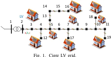
Fig. 1. Cigre LV grid.
becomes one when the inside statement is true. Finally, x˜0
is the model intercept and γ a parameter which updates the location of the breakpoints towards the optimal one. Then, we update the breakpoints s¯i¯k+1 =
γ¯k β¯k +s
¯i ¯
k and iteration index ¯i = ¯i+ 1, repeating the procedure until the RSS does not change between two iterations.
The same method is used both for the APC and RPC curves, using respectively the PV optimal active and reactive setpoints from the OPF in Section II.
2) C2: This scheme extends the model presented in Section III-A2 to account also for local voltages, resulting in a feedback control scheme. More specifically, the updated feature matrices areΦ(j)6 = [Φ(j)2, φ(j)
8,t]T,Φ (j)
7 = [Φ
(j)
3, φ
(j)
8]T and
Φ(j)8 = [Φ(j)4, φ(j)
8]T and are used in (8), (9) and (10) to derive
the regression coefficients for this dynamic control scheme.
IV. CASESTUDY- RESULTS
A. Network description - Case study setup
To demonstrate the performance of the four methods, we use the benchmark radial residential LV grid presented in [22] and shown in Fig. 1. The load and PV panels are distributed to the three phases unevenly, resulting in unbalanced conditions. The total load, taken from [22], is shared 25%-60%-15% among the three phases. The installed PV capacity, is set to SPV
rated= 150% of the total maximum load of the entire feeder to the PV nodes= [3,5,7,10,12,16,17,18,19], and is shared25% -25%-50% among the three phases.
In the design stage, we use the algorithm in Section II to process a 30-day summer dataset with forecasts of load and PV production, and generate the optimal DER setpoints. The operational costs of the centralized problem are assumed to be cP = 0.3CHFkWh and cQ = 0.01·cP. From the optimal DER
data, we derive the three data-driven schemes (O1, C1, C2) as described in Section III. Then, we evaluate their performance, and compare it to O1 and the optimal (OPF-based), using data from another summer month. The implementation was done in MATLAB using YALMIP [23] as the modeling layer and Gurobi [24] as the solver. The results were obtained on an Intel Core i7-2600 CPU and 16 GB of RAM.
B. Derived local control schemes
1) Local open-loop control:
0 0.2 0.4 0.6 0.8 1 0.85
0.9 0.95 1
Pgen(p.u.)
P
ow
er
fac
tor
(-)
[image:6.612.63.285.49.147.2]S<13.8 kVA S>13.8 kVA
Fig. 2. Open-loop power factor adjustment.
b) O2: Figure 3 shows the boundaries for APC activation. As it is expected, PV generation above a certain threshold, i.e. φ191 ≈ 0.8 p.u. in this case, would lead to
power quality issues, e.g. overvoltages or thermal overloads. However, at high (low) levels of local load (φ197 ), the boundary
threshold value increases (decreases), since more (less) active power can be consumed by the local load.
2) Local closed-loop control:
a) C1: Figure 4 presents the local volt-var character-istic curves derived according to Section III-B1 of all PV units in phase C. Node 3 injects reactive power to optimize losses, while the remaining nodes absorb reactive power at voltages smaller than the maximum acceptable value of 1.04p.u..
b) C2: As described in Section III-A2, regression models are calculated for each DER unit using the feature-matrix Φ2 for the open-loop O2 and Φ6 for the closed-loop C2 scheme, respectively. Table I shows the dominant features for both cases, for all phases at Node 3 (close to the substation) and at Node 19 (at the end of the feeder). In contrast to [11], here the behavior of the DERs is based mostly on the inverter maximum capacity (φ4). Phases a
andb do not face overvoltage or overloading challenges, and thus, they show a capacitive behavior injecting reactive power to optimize losses. On the other hand, Phase c, hosting the biggest share of PV units, shows inductive behavior at hours with high solar radiation to reduce voltages.
C. Method Comparison
[image:6.612.315.564.51.165.2]In this section, we investigate the ability of open- and closed-loop local schemes to emulate the centralized behavior. First, we consider operating conditions similar to the training dataset. Second, we explore the robustness of the schemes
Fig. 3. Active power curtailment (APC) classification regions for the real -time response of the DER based on local load and PV generation.
0.9 0.95 1 1.05 1.1
−1
−0.5 0 0.5 1
Voltage magnitude (p.u) Qg
/Q
m
a
x
(p
.u
.)
[image:6.612.61.292.552.694.2]3 5 7 10 12 16 17 18 19
Fig. 4. Individual local characteristic curves for reactive power control of the PV units at phase C.
TABLE I
NORMALIZED COEFFICIENT OF THE DOMINANT FEATURE ATNODE19. Dominant Feature
O2 C2
Node 3 Node 19 Node 3 Node 19 Phase a φ4 φ2 φ4 φ8
Phase b φ4 φ2 φ4 φ4
Phase c φ2 φ4 φ4 φ4
when the given inputs are significantly different from the training sets, providing some insights on a safety issue of AI-based control methods.
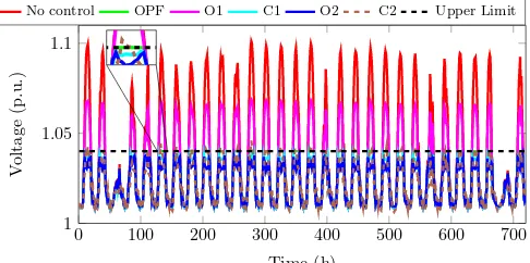
1) Expected operating conditions: Table II summarizes the results in terms of losses, highest voltage and thermal load-ing, and the needed active power curtailment from applying all methods in real-time operation for a period of one summer month (different from the one used in the training stage). As can be seen, the OPF satisfies all security constraints. Method O1 (standard industry practice) results in higher maximum loading due to increased needs for reactive power by the PV units, without solving the overvoltage issue. Methods O2, C1 and C2 mitigate adequately the power quality issues with marginal violations which are acceptable by grid codes, while being capable of mimicking satisfactorily the OPF-based control without the need of communication. This can be seen also in Fig. 5 that shows the voltage magnitude evolution of Node 19, the worst in terms of maximum voltage node.
2) Robustness to different conditions: Here we use the same seasonal characteristics, but the network has changed by installing a new PV unit, or connecting an additional load. These conditions were not seen in the training data, and the focus here is to assess how the controllers will behave under an unseen setup without re-training. In order to examine the
0 100 200 300 400 500 600 700
1 1.05 1.1
Time (h)
V
ol
tage
(p
.u
.)
No control OPF O1 C1 O2 C2 Upper Limit
[image:6.612.319.562.583.704.2]TABLE II
SUMMARIZED MONTHLY RESULTS FOR ALL METHODS(ONLY THE LARGEST OBSERVED VALUE IS LISTED)
Method No control OPF O1 C1 O2 C2 Losses (%) 4.19 4.82 4.602 3.722 4.475 4.812
|V|max(p.u.) 1.09 1.04 1.069 1.039 1.038 1.042
|I|max(%) 112 100 119.9 91.5 104.2 101.5
Pc(%) 0 0.96 0 4.93 1.16 1.18
locational impact, we consider two locations for these changes; that is, at Node 4 - close to the secondary of the transformer, and at Node 11 - almost at the end of the feeder, both at phase C. The added PV unit and load are chosen as 50% of the respective values of PV capacity and load of Node19.
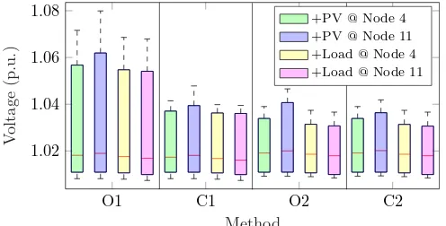
Figure 6 shows the boxplots (minimum, first quartile, me-dian, third quartile, and maximum values) for the monthly voltage magnitude at Phase C of Node 19, for all methods. In all cases, adding a PV unit at Node 11 (away from the substation) results in higher grid voltages, compared to Node 4which is close to the transformer where voltage is regulated. As with the previous tests, method O1 is the most inefficient, imposing a certain behavior to all DGs. Methods C1, O2 and C2 behave satisfactorily, with overvoltages only when adding a PV at Node 11. In this case, Method C2 achieves the best performance since it reacts to the measured voltage, although the change has occurred elsewhere in the grid. This highlights the benefit of method C2, since voltage inherently brings global information through the physics of the system. Finally, the two load cases are similar, because the amount of load that is added is relative low and does not influence the voltages significantly.
V. CONCLUSION
In the future, active DNs will rely on controlling DERs to ensure a safe, reliable and optimal operation of the grid. On the one hand, centralized, OPF-based controllers achieve optimal results, but rely on communication and monitoring infrastructure. On the other hand, local schemes are robust and inexpensive, but cannot cope efficiently with the modern challenges of DNs. In this paper, we examine data-driven local control schemes, trained off-line to mimic the central-ized optimal behavior without the need for monitoring and communication infrastructure. We revisited existing methods, proposed a new variation (C2), and compared in terms of performance under normal and unseen conditions. Future work
O1 C1 O2 C2
1.02 1.04 1.06 1.08
Method
V
ol
tage
(p
.u
.)
[image:7.612.53.301.569.695.2]+PV@Node4 +PV@Node11 +Load@Node4 +Load@Node11
Fig. 6. Boxplots of the voltage magnitudes for all methods when a new PV unit or load is installed at Node 19, phase C.
will focus on the inclusion of safety constraints in the design stage of such controllers.
REFERENCES
[1] N. Hatziargyriou, O. Vlachokyriakou, T. Van Cutsem, J. Milanovi´c, P. Pourbeik, C. Vournas, M. Hong, R. Ramos, J. Boemer, P. Aristidou, V. Singhvi, J. dos Santos, and L. Colombari, “IEEE PES Task Force on Contribution to Bulk System Control and Stability by Distributed Energy Resources connected at Distribution Network,” Tech. Rep., 2017. [2] J. Lavaei and S. H. Low, “Zero duality gap in optimal power flow
problem,”IEEE Trans. on Power Systems, vol. 27, no. 1, pp. 92–107, 2012.
[3] P. Fortenbacher, M. Zellner, and G. Andersson, “Optimal sizing and placement of distributed storage in low voltage networks,” inProc. of the 19th PSCC, Genova, Jun 2016.
[4] S. Karagiannopoulos, P. Aristidou, A. Ulbig, S. Koch, and G. Hug, “Op-timal planning of distribution grids considering active power curtailment and reactive power control,”IEEE PES General Meeting, 2016. [5] P. Kotsampopoulos, N. Hatziargyriou, B. Bletterie, and G. Lauss,
“Review, analysis and recommendations on recent guidelines for the provision of ancillary services by Distributed Generation,” in IEEE International Workshop on Intelligent Energy Systems, IWIES, 2013. [6] S. Bolognani and S. Zampieri, “A distributed control strategy for
reactive power compensation in smart microgrids,”IEEE Transactions on Automatic Control, vol. 58, no. 11, pp. 2818–2833, Nov. 2013. [7] A. Garg, M. Jalali, V. Kekatos, and N. Gatsis, “Kernel-Based
Learning for Smart Inverter Control,” 2018. [Online]. Available: http://arxiv.org/abs/1807.03769
[8] O. Sondermeijer, R. Dobbe, D. Arnold, and C. Tomlin, “Regression-based Inverter Control for Decentralized Optimal Power Flow and Voltage Regulation,”IEEE PES General Meeting, 2016.
[9] S. Karagiannopoulos, P. Aristidou, and G. Hug, “Hybrid approach for planning and operating active distribution grids,”IET Generation, Transmission & Distribution, pp. 685–695, Feb 2017.
[10] S. Karagiannopoulos, P. Aristidou, and G. Hug, “Data-driven Local Control Design for Active Distribution Grids using off-line Optimal Power Flow and Machine Learning Techniques,” Accepted in IEEE Transactions on Smart Grid, 2019, doi: 10.1109/TSG.2019.2905348. [11] R. Dobbe, O. Sondermeijer, D. Fridovich-Keil, D. Arnold, D. Callaway,
and C. Tomlin, “Data-Driven Decentralized Optimal Power Flow,” 2018. [Online]. Available: http://arxiv.org/abs/1806.06790
[12] F. Bellizio, S. Karagiannopoulos, P. Aristidou, and G. Hug, “Optimized local control schemes for active distribution grids using machine learning techniques,” inIEEE PES General Meeting 2018, June 2018. [13] S. Karagiannopoulos, P. Aristidou, and G. Hug, “Co-optimisation of
Planning and Operation for Active Distribution Grids,” inProc. of the 12th IEEE PES PowerTech, Manchester, Jun 2017.
[14] D. Amodei, C. Olah, J. Steinhardt, P. Christiano, J. Schulman, and D. Man´e, “Concrete Problems in AI Safety,” 2016. [Online]. Available: http://arxiv.org/abs/1606.06565
[15] S. Karagiannopoulos, P. Aristidou, and G. Hug, “A Centralised Control Method for Tackling Unbalances in Active Distribution Grids,” inProc. of the 20th PSCC, Dublin, June 2018.
[16] J. H. Teng, “A direct approach for distribution system load flow solutions,”IEEE Trans. on Power Delivery, vol. 18, pp. 882–887, 2003. [17] S. Karagiannopoulos, P. Aristidou, L. Roald, and G. Hug, “Operational Planning of Active Distribution Grids under Uncertainty,” inIREP 2017, X Bulk Power Systems Dynamics and Control Symposium,, Aug 2017. [18] W. H. Kersting,Distribution System Modeling and Analysis, 2002. [19] VDE-AR-N 4105, “Power generation systems connected to the LV
distribution network.” FNN, Tech. Rep., 2011.
[20] IEEE 1547, “IEEE Standard for Interconnecting Distributed Resources with Electric Power Systems,” Jul 2003.
[21] V. M. R. Muggeo, “Estimating regression models with unknown break-points,”Statistics in Medicine, vol. 22, no. 19, pp. 3055–3071, Oct 2003. [22] K. Strunz, E. Abbasi, C. Abbey, C. Andrieu, F. Gao, T. Gaunt, A. Gole, N. Hatziargyriou, and R. Iravani, “Benchmark Systems for Network Integration of Renewable and Distributed Energy Resources,”CIGRE, Task Force C6.04, no. 273, pp. 4–6, 4 2014.
[23] J. L¨ofberg, “Yalmip : A toolbox for modeling and optimization in matlab,” inProc. of the CACSD Conference, Taiwan, 2004.