Efficient reconstruction of constrained MSSM parameters from LHC data: A case study

(1)

promoting access to White Rose research papers

Universities of Leeds, Sheffield and York

http://eprints.whiterose.ac.uk/

This is an author produced version of a paper published in

Physical Review D

.

White Rose Research Online URL for this paper:

Published paper

Roszkowski, L., Ruiz de Austri, R., Trotta, R. (2010)

Efficient reconstruction of

constrained MSSM parameters from LHC data: A case study

Physical Review D,

82 (5), Art. no.055003

(2)

arXiv:0907.0594v2 [hep-ph] 3 Sep 2010

Efficient reconstruction of CMSSM parameters from LHC data –

A case study

Leszek Roszkowskia1,Roberto Ruiz de Austrib2, andRoberto Trottac3

a _{Department of Physics and Astronomy, University of Sheffield, Sheffield, S3 7RH, UK, and}

The Andrzej Soltan Institute for Nuclear Studies, Warsaw, Poland

b _{Instituto de F´ısica Corpuscular, IFIC-UV/CSIC, Valencia, Spain}

c _{Astrophysics Group, Imperial College, Blackett Laboratory, Prince Consort Road, London SW7}

2AZ, UK

Abstract

We present an efficient method of reconstructing the parameters of the Constrained MSSM from assumed future LHC data, applied both on their own right and in combination with the cosmological determination of the relic dark matter abundance. Focusing on the ATLAS SU3 benchmark point, we demonstrate that our simple Gaussian approximation can recover the values of its parameters remarkably well. We examine two popular non-informative priors and obtain very similar results, although when we use an informative, naturalness-motivated prior, we find some sizeable differences. We show that a further strong improvement in reconstructing the SU3 parameters can by achieved by applying additional information about the relic abundance at the level of WMAP accuracy, although the expected data from Planck will have only a very limited additional impact. Further external data may be required to break some remaining degeneracies. We argue that the method presented here is applicable to a wide class of low-energy effective supersymmetric models, as it does not require to deal with purely experimental issues, e.g., detector performance, and has the additional advantages of computational efficiency. Furthermore, our approach allows one to distinguish the effect of the model’s internal structure and of the external data on the final parameters constraints.

1

[email protected] 2

[email protected] 3

(3)

1 Introduction

If softly broken low-energy supersymmetry (SUSY) provides a correct description of the particle physics realm at energy scales around a few hundred GeV and above, then superpartners are likely to be discovered at the LHC. One of the main goals of ATLAS and CMS experiments will be to identify those particles by determining their masses and other properties.

The actual outcome will depend not only on the LHC machine and detector performance but obviously also on the mass scales of the superpartners themselves. A whole plethora of different possibilities can be listed here, ranging from one extreme where all of the superpartners may come out to be too heavy to for the LHC reach, to another where all, or most, of them will be discov-ered. Unfortunately, basically the whole spectrum of options remains open even in perhaps the most economical SUSY framework, the Constrained Minimal Supersymmetric Model (Constrained MSSM, or CMSSM) [1] which includes the minimal supergravity (mSUGRA) model [2], as shown by a number of recent global fits of the CMSSM based on Bayesian statistics [3, 4] and on a χ2

approach [5, 6]. While the latter show a stronger preference for a fairly low SUSY mass scale, in the range of a few hundred GeV, the former point to a more cautious picture, where a much wider mass range remains allowed. This discrepancy is caused by the fact that, with the data that is currently available, even the CMSSM still remains to some extent underconstrained, and the specifics of the statistical and data analysis treatment can lead to fairly different results. It is therefore clear that selecting, or at least limiting, SUSY models by using LHC measurements is certainly going to be a very challenging task as there exist large degeneracies among the MSSM parameters that can lead to indistinguishable LHC signatures (see, e.g., Ref. [7]).

In preparation for dealing with real data, a number of approaches to particle mass reconstruction have been developed based on extracting kinematic information from one or more decay chains of superpartners, typically requiring two or more visible particles in the final state [8]. These and other techniques have been used by LHC experimental groups which have performed a large number of detailed studies in a few reference, or “benchmark”, points, often selected in such a way as to typically allow several of the superpartners to be seen at the LHC.

In a recent extensive ATLAS Report [9], in the framework of the CMSSM/mSUGRA a so-called ATLAS SU3 benchmark point (which is specified below) was examined with Markov Chain Monte Carlo (MCMC) scans, with the aim of evaluating the expected accuracy of reconstructing CMSSM parameters: a common gaugino mass parameter m1/2, a common scalar mass parameter m0, a

common trilinear term A0, all evaluated at the unification scale MGUT ≃ 2×1016 GeV, plus a

Higgs vacuum expectation values tanβ. Assuming an integrated luminosity of 1 fb−1_{, a dilepton}

and lepton+jets edge analysis of the decay chain qeL → χ02(→ el±l∓)q → χ01l+l−q and the high-pT

and large missing energy analysis of the decay chain qeR → χ01q were performed, where eqL (eqR)

denotes the first or second generation left (right) squark, χ0

1,2 the first and second neutralino andel

an intermediate slepton. It was concluded thatm1/2 and m0 could be reconstructed with adequate

accuracy, while prospects for tanβ looked somewhat poorer, and even more so forA0 (see Ref. [9],

pp. 1617, ff).

(4)

likelihood is sufficient to reproduce with reasonable accuracy the results of the full ATLAS analysis, while being much more economical in terms of computational requirements, when we use the same linear, or flat (as defined below) prior. We then build on the ATLAS analysis by examining the impact of two other priors. We find that non-informative priors (i.e., priors whose characteristic scale is much larger than the support of the likelihood) lead to approximate prior-independence in the posterior, thus significantly improving with respect to the current situation. On the other hand, if one imposes extra theoretical prejudice in the prior (by choosing a prior that penalizes fine-tuning), the posterior is still quite strongly affected.

We also compare with the limits that can be obtained using a maximum likelihood analysis, and we show that the choice of statistics (Bayesian or maximum likelihood) no longer matters once one combines ATLAS data with cosmological relic abundance determinations. We clarify what rˆole is played by assuming a specific theoretical model (here the CMSSM) in complementing the information coming from the ATLAS measurements with model-specific theoretical correlations between masses of the observables.

In the second step, we go beyond the ATLAS analysis by applying additional information about the cosmological relic density Ωχh2 of the lighest neutralino χ01 (below often denoted by χ for

simplicity), assumed to be dark matter (DM) in the Universe. The dark matter abundance clearly provides additional information about the model at hand, and in this analysis we aim at obtaining a quantitative measure for the extra constraining power that it provides, on top of that expected from the ATLAS data. Here we first impose WMAP uncertainties on Ωχh2 and demonstrate a significant

improvement in the determination of the CMSSM parameters, especially m0. Next we investigate

the impact of further reducing the observational errors on Ωχh2 to an accuracy as expected from

Planck, and show that this will lead to only a further modest improvement. We also comment on the impact of some other commonly used constraints, in particular fromb→sγ and (g−2)µ, which

we, however, do not apply here. Finally, we examine the impact of the different constraints from ATLAS and cosmology on the uncertainties of mass measurements of several superpartners and on predictions for the scattering cross section relevant for direct detection of dark matter experiments. The paper is organized as follows. In Sec. 2 we present a setup of our analysis for the ATLAS SU3 point in the CMSSM, including details of our scans of the CMSSM parameters. In Sec. 3 we present our numerical results for the posterior probability density functions (pdfs), including a discussion of an impact of adding further assumptions and information. In Sec. 4 we compare some of these with the alternative measure of the profile likelihood. We summarize our findings in Sec. 5.

2 Setup and benchmark point

2.1 The ATLAS SU3 benchmark point

(5)

CMSSM parameter ATLAS SU3 benchmark value SM parameter Input value

m1/2 300 GeV Mt 172.6 GeV

m0 100 GeV mb(mb)M S 4.20 GeV

tanβ 6.0 αs(MZ)M S 0.1176

A0 −300 GeV 1/αem(MZ)M S 127.955

[image:5.612.94.499.233.365.2]

sgn(µ) +

Table 1: Left side: input CMSSM parameters values for the ATLAS SU3 benchmark point. Right side: input values of relevant SM parameters used in the numerical analysis.

superpartner mass superpartner mass superpartner mass

χ0

1(=χ) 117.9 GeV eeL,eµL 230.8 GeV deL 666.2 GeV

χ0

2 223.4 GeV eeR,µeR 157.5 GeV deR 639.0 GeV

χ0

3 463.8 GeV eνe,νeµ 217.5 GeV ueL 660.3 GeV

χ0

4 479.9 GeV eτ1 152.2 GeV ueR 644.3 GeV

χ+₁ 224.4 GeV eτ2 232.4 GeV eb1 599.0 GeV

χ+₂ 476.4 GeV _eντ 216.9 GeV eb2 636.6 GeV

e

g 717.5 GeV et1 446.9 GeV

e

t2 670.9 GeV

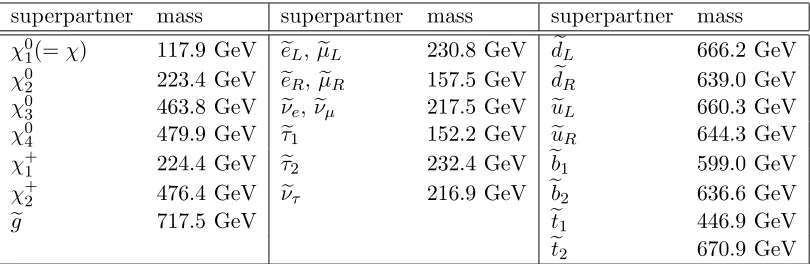
Table 2: Superpartner mass spectrum for the ATLAS SU3 point.

Since LHC data is rather unlikely to differentiate among the flavors of the squarks of the first two generation, in what follows we denote them all by a common symbolq_e, and bym_e_qtheir average mass, similarly as in Ref. [9]. On the other hand,el will denote the lightest slepton andm_e_l its mass. In the case of the ATLAS SU3 point its rˆole is played byeτ1.

The resulting mass spectrum, as computed using the SoftSusy code version 1.0.18 [10] in the 1-loop approximation is given in Table 2. By comparing with the mass spectrum for the ATLAS SU3 point given in Ref. [9] (cf. Table 2 on page 1516), we can see some differences, especially a systematic shift in squark masses by a few tens of GeV, which may be due to using different numerical codes, approximations (although in both cases 1 loop expressions are applied) as well as different inputs in SM parameter values. While this will contribute to some differencies we will find with the ATLAS results, at the end these discrepancies are of secondary importance, as we discuss below.

2.2 The likelihood function

The study performed by the ATLAS Collaboration on the SU3 point reports the expected accuracy in the reconstruction of some of the masses and mass differences in the benchmark SUSY spectrum given in Table 2. Dilepton edges will constrain m_χ0

1, mχ 0

2, meq and mel with fairly poor accuracy,

(6)

In the case of the SU3 point considered here, the two-body decay channel χ0

2 → el±l∓ dominates,

sincem_χ0

2 > mel, and the distribution of the invariant mass of the two leptons is triangular, with an

endpoint given by [9] (p. 1619)

medge=m_χ0 2

v u u

t₁₋ mel

m_χ0 2

!2s

1−

_m

χ0 1

m_e_l

2

. (1)

A measurement of the dilepton endpoint leads to a relationship between χ0

2, χ01 and the slepton

involved. Further mass distributions are considered in order to determine the masses of all the particles involved in the process, as described in Ref. [9] (pp. 1619, ff), along with event and cut selection procedures adopted in a reconstruction of the dilepton and other edges.

The observable quantities to be constrained by ATLAS are given by the set

θ={m_χ0 1, mχ

0 2 −mχ

0

1, mel−mχ 0

1, meq−mχ 0

1}. (2)

We further assume that the maximum likelihood (ML) value of θ obtained by ATLAS, θML,

cor-responds to the value of the true benchmark point, θ⋆={117.9,105.5,34.3,534.5} GeV, where the

numerical value is obtained from Table 2. In other words, we neglect realization noise, an assump-tion which is justified by the fact that hθMLi =θ⋆, whereh·i denotes an average over realizations.

The likelihood function from ATLAS is then modeled as a Gaussian centered around the true value of the observable quantities,

−2 lnLATLAS=χ2ATLAS= (θ−θML)tC−1(θ−θML), (3)

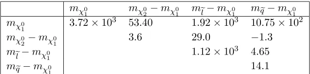
where the covariance matrixCis given in Table 3 (and we have dropped an irrelevant normalization constant). It represents the full covariance between the masses and the mass differences. The covariance matrix includes statistical errors only; systematic errors are negligible.

The form of the ATLAS likelihood function given in Eq. (3) is a simple Gaussian approximation to the actual likelihood function that one would obtain from a full analysis of simulated ATLAS data. The latter is, however, not available outside the Collaboration, and therefore our approximation represents the best that can be reasonably done given the information that is expected to be publicly available. There are two reasons why it might be interesting to consider an approximate ATLAS likelihood function at the level of the SUSY mass spectrum. Firstly, it is not unreasonable that the simple approximation adopted here will give a fairly accurate representation of ATLAS capabilities (see below for further comments on how this compares with the full analysis carried out by the ATLAS Collaboration), and therefore provide a useful shortcut to quantitatively implementing the constraints that would result from a full analysis. Secondly, given the model-independent constraints on the low-energy SUSY mass spectrum, one can use them to constrain the high-energy parameters of any SUSY model of the MSSM class, in this case the CMSSM. As we shall show below, the constraining power included in the low-energy likelihood is then supplemented by the theoretical structure of the model itself.

(7)

m_χ0

1 mχ

0 2−mχ

0

1 mel−mχ 0

1 meq−mχ 0 1

m_χ0

1 3.72×10

3 ₅₃_.₄₀ ₁_.₉₂_×₁₀3 ₁₀_.₇₅_×₁₀2

m_χ0 2−mχ

0

1 3.6 29.0 −1.3

m_e_l−m_χ0

1 1.12×10

3 ₄_.₆₅

mq_e−mχ0

[image:7.612.138.454.99.175.2]

1 14.1

Table 3: ATLAS covariance matrix employed in the analysis.

• ATLAS data only: including only the likelihood function given by Eq. (3);

• ATLAS data (as above) + WMAP-level uncertainty on dark matter abundance;

• ATLAS data (as above) + Planck-level uncertainty on dark matter abundance.

When including information about the cosmological dark matter abundance, we have to address the fact that the value of the neutralino relic abundance (computed using the code Micromegas [11]) for the ATLAS SU3 benchmark point, is Ωχh2 = 0.2332, which is a factor of some 2.5 above the

WMAP range of 0.1099±0.0062 for the cosmological dark matter [12]. However, assuming standard Big Bang cosmology and that the CMSSM is correct, we would expect that for the actual measured value of the CMSSM parameters, for which ATLAS and/or CMS measurements are made, Ωχh2

would lie in the WMAP range. It is therefore not unreasonable to examine the impact of the extra piece of information, both in terms of its value and uncertainty, which is provided by the cosmological relic density of dark matter. Notice that we do not rely here on a potential ability to reconstruct Ωχh2 from LHC data alone [13] (which, on the other hand, could provide an important

cross-check of our cosmological input) but use it as external constraint. Therefore, since the ATLAS analysis has been carried out for the ATLAS SU3 point, with the specific values of the CMSSM parameters, we also adopt to keep this central value for the relic abundance. On the other hand, we don’t expect any major change in the numerical results presented below if Ωχh2 were actually

close to the WMAP range.

In our analysis we implement the cosmological dark matter determination as follows. Firstly, we assume that the true value of the relic abundance corresponds to the value computed for the benchmark point, and that WMAP-level constraints correspond to a Gaussian likelihood cen-tered around that value with standard deviation given by the current WMAP uncertainty, namely

σWMAP = 6.2×10−3:

−2 lnLWMAP=χ2WMAP=

(Ωχh2−0.2332)2

σ2 WMAP

. (4)

The Planck satellite is expected to improve the WMAP accuracy on the relic abundance by a factor

∼10 [14]. When including Planck-level constraints, we therefore adopt the same likelihood as above but with a smaller standard deviation,σPlanck = 6.2×10−4. Since for the “bulk region” to which the

ATLAS SU3 point belongs the theoretical error in the relic abundance is estimated to be tiny [15] we neglect it here. In other cases it can be much larger, primarily due to the larger uncertainties in computing mass spectra; for example in the focus point region it would likely dominate and this would cloud the potential impact of the cosmological data.

(8)

any other constraints, e.g., from LEP, rare processes in heavy quark physics (b → sγ, etc) or the anomalous magnetic moment of the muon (g−2)µ, which are routinely used in global analyses

of the CMSSM and other popular SUSY models. We have also checked that fixing the nuisance parameters or marginalising over them has a negligible impact on the results. Therefore we only present results with the nuisance SM parameters fully marginalised, even though in the ATLAS analysis the SM parameters were fixed at their central values.

2.3 Scanning the CMSSM parameters

With the aim of reconstructing the true values of the defining parameters for the ATLAS SU3 point, we explore the CMSSM parameter space with the help of the Nested Sampling (NS) scanning technique, as implemented in the MultiNest algorithm [16].

We consider two different non-informative priors, that is, priors which contain minimal assump-tions about the values of the parameters:

• flat prior: flat in m1/2, m0, A0,tanβ, with the ranges: 50 GeV ≤ m1/2, m0 ≤ 500 GeV,

2≤tanβ ≤62 and −4 TeV≤A0 ≤4 TeV.

• log prior: flat in logm₁_/₂,logm0, A0,tanβ, with the same ranges: log(50)≤logm0,logm1/2≤

log(500) (in GeV), and as above forA0 and tanβ.

Notice that we have employed here narrower ranges of m1/2 and m0 than the values of up to

a few TeV used in our previous analyses [4, 18]. However, we have checked that enlarging the prior range to much larger values of m1/2, m0 (up to 4 TeV) has no impact on our reconstructed

parameter values, as our algorithm correctly recovers the true parameter values even in the case of a much larger prior range. Finally, for the SM nuisance parameters we assume the same ranges as in our previous papers [4, 18]; in any case as we have mentioned above, the details of the treatment of nuisance parameters has basically no impact on the results presented here.

One of the aims of this work is to demonstrate that ATLAS data will achieve approximate prior-independence for the two choices of non-informative priors given above, which have been widely used in the literature so far and for which it has been shown that the current posterior for the CMSSM retains a fairly substantial prior dependence [18]. However, while this is encouraging, clearly that does not imply that one should expect the same to hold with any other choice of prior, of which there is an infinite range. Furthermore, in the Bayesian framework it is always possible to supplement the information contained in the likelihood by external prior information, for example by imposing “naturalness” constraints [20, 17]. In this case, one would not expect the posterior to remain independent of the prior, but actually to show stronger constraints than for the case of non-informative priors. In order to investigate to what extent a “naturalness” prior can supplement ATLAS data in constraining CMSSM parameters, we also consider an informative prior choice in section 3.4, with the following “CCR prior” (after Cabrera, Casas and Ruiz de Austri, who introduced it) [20],

• CCR prior: flat onm0, m1/2, A0, Bbut with an effective “penalty term” that naturally leads

to low fine tuning among SUSY parameters.

(9)

more fundamental. On the other hand, for the purpose of performing a numerical scaning of the model parameter space it is much more convenient to trade some of them for the CMSSM param-eters which have a more direct phenomenological significance. (In addition one has the usual SM nuisance parameters.) In Refs. [20, 21] it has been shown that it is convenient to replace µ with

mZ, which is trivially integrated out. In addition, this procedure automatically takes into accounts

the usual measure [22, 23] of the degree of fine-tuning. Furthermore, it is also convenient to trade theB parameter for the derived quantity tanβ.

The change of variables{µ, B} → mZ,tanβleads to theeffective priorin the CMSSM variables

peff(m0, m1/2, A0,tanβ) ≡ J|µ=µZ p(m0, m1/2, A0, B, µ=µZ), (5)

where p(m0, m1/2, A0, B, µ = µZ) the prior for the mSUGRA parameters and J is a Jacobian of

the transformation, which is evaluated in the usual way from minimization equations of the Higgs scalar potential, V(H1, H2). This way one arrives at an approximate form for the effective prior [20]

peff(m0, m1/2, A0,tanβ) ∝

tan2_β₋₁

tan2_β_{(1 + tan}2_β₎

Blow

µZ

p(m0, m1/2, A0, B, µ=µZ) , (6)

whereBlowis the parameterBevaluated at the electroweak scale andµZis chosen so that it gives the

correct ofmZ. The CCR prior is then defined as the effective priorpeff(m0, m1/2, A0,tanβ), Eq. (6),

where we take a flat prior in m0, m1/2, A0, B and µ.

3 Results

In this Section we present our numerical results from scans performed using the publicly avail-able SuperBayes package version 1.35 [24], which we have modified in order to include a Gaussian likelihood from projected ATLAS data as described above.

3.1 Using ATLAS data only and non-informative priors

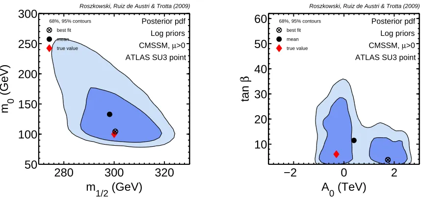
We begin by considering the constraining power on the CMSSM parameters of ATLAS mass spec-trum data alone. In Figs. 1 and 2 we present 2-dimensional (2D) Bayesian posterior pdfs assuming the log and the flat prior, respectively, while the corresponding 1D pdfs for the log prior case are shown in Fig. 3. By examining the (m1/2, m0) plane for the log prior in Fig. 1, we can see that

both the 68% (inner regions) and the 95% (outer regions) total probability regions are well centered around the true value. Our algorithm recovers the best-fit point within the limits of numerical noise for all CMSSM parameters, except for A0, where the reconstructed best-fit ends up in a wrong

re-gion of the parameter space due to a fundamental degeneracy discussed below. The posterior mean is also reasonably close to the true value (within 1σ for all parameters, except for A0), although it

is slightly skewed due to the asymmetric nature of the contours, which exhibit heavier tails than Gaussian (see also Fig. 3 below). On the other hand, tanβ is somewhat less well reconstructed, yielding only an upper limit.

In contrast, A0 is rather poorly constrained in this case, and actually shows a sign ambiguity.

(10)

m

1/2 (GeV)

m 0

(GeV)

Roszkowski, Ruiz de Austri & Trotta (2009)

68%, 95% contours best fit mean true value

Posterior pdf Log priors CMSSM, µ>0 ATLAS SU3 point

280 300 320

50 100 150 200 250 300

A

0 (TeV)

tan

β

−2 0 2

[image:10.612.80.510.108.318.2]

10 20 30 40 50 60

Figure 1: 2D posterior pdf for the case of applying ATLAS mass spectrum data alone, for some CMSSM parameter combinations and for the log prior choice. Compare with Fig. 12, p. 1638 of [9].

Xτ =Aτ−µtanβ in the stau mass matrix, whereAτ is the value ofA0 at the EW scale evaluated

with its RGE and µ is computed from the usual requirement of correct electroweak symmetry breaking. A closer examination reveals that, for A0 ∼ 1 TeV (in between the two 1σ regions in

the right panel of Fig. 1),Xτ is minimized and the mass difference betweenτe2 and eτ1 (which plays

the rˆole of the lightest slepton in the decay chain) goes to zero. Since in the ATLAS analysis only

e

τ1 was considered, such cases are not allowed. Our study thus reveals that in studying the decay

χ0

2 →el±l∓→χ01l+l− the exchange of botheτ2 andτe1 should be considered, as for some values ofA0

their masses, and therefore also relative contributions, may be comparable.

In the case of the flat prior (Fig. 2) the emerging picture remains essentially identical, thus confirming that the prior choice becomes less of an issue once the constraining power of the data is sufficiently strong, as expected. Many of the features seen in Fig. 1 are displayed more clearly in Fig. 3 where the corresponding 1D pdfs are presented for the log prior case only; the flat prior produces very similar results and is therefore not shown. We give the 68% and 95% intervals of our reconstructed CMSSM parameters in Table 4. A comparison with the profile likelihood is carried out further below.

When considering posterior constraints on the SUSY mass spectrum, it is apparent that some of the constraints are much stronger than the likelihood function alone (which actually applies to a more general case of the MSSM) would seem to imply. For instance, the 1σ error on m_χ0 1

(11)

m

1/2 (GeV)

m 0

(GeV)

Posterior pdf Flat priors CMSSM, µ>0 ATLAS SU3 point

280 300 320

50 100 150 200 250 300

A

0 (TeV)

tan

β

Posterior pdf Flat priors CMSSM, µ>0 ATLAS SU3 point

−2 0 2

[image:11.612.80.509.108.318.2]

10 20 30 40 50 60

Figure 2: The same as in Fig. 1 but for the flat prior case. Notice that the two choices of priors lead to statistically indistinguishable results.

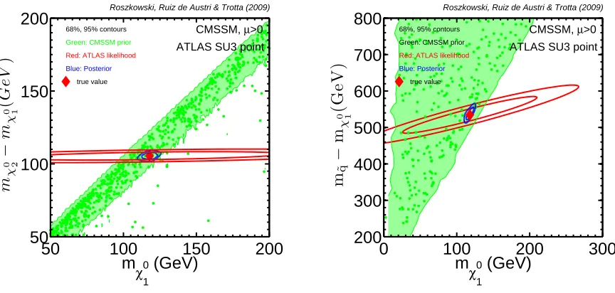
the CMSSM shows a much smaller error, of order ∼ 4 GeV, cf. Table 4. The reason for this is that the information supplied by the likelihood is supplemented by the internal structure of the CMSSM parameter space, within which the masses of many of the sparticles are highly correlated. This is demonstrated in Fig. 4, where one can see that the correlation between masses in the spectrum within the CMSSM is nearly orthogonal to the constraints provided by ATLAS for the mass spectrum observables plotted in the Figures. One can think of this correlation as an additional

a prioripiece of information contained in the model. In other words, given the theoretical structure

of the CMSSM, certain mass combinations in the spectrum (which are otherwise allowed by the projected ATLAS constraints, red ellipses in Fig. 4) are simply not allowed by the structure of the model. Therefore the final constraints on the spectrum are much tighter than the likelihood alone would imply. Supplementing the mass spectrum constraints with a model-specific implementation, as done here, has the additional advantage of displaying which part of the constraining power comes from the experimental data and which one from the theoretical properties of the model.

It is interesting to examine how well our procedure allows one to use the assumed ATLAS data alone to determine the relic abundance for the ATLAS SU3 point, in some analogy with what, for example, has been done for some other benchmark points in Refs. [13, 25]. This is shown in Fig. 5 where we find that, from the assumed ATLAS data alone one would obtain Ωχh2 = 0.253±0.034,

(12)

m

0 (GeV)

Probability

100 200 300

0 0.2 0.4 0.6 0.8 1

m

1/2 (GeV)

Probability

280 300 320

0 0.2 0.4 0.6 0.8 1

A

0 (TeV)

Probability

−2 0 2

0 0.2 0.4 0.6 0.8 1

tan β

Probability

20 40 60

[image:12.612.87.514.113.553.2]

0 0.2 0.4 0.6 0.8 1

(13)

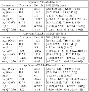
Applying ATLAS data only Parameter True value Best fit 68% (95%) range

m1/2 (GeV) 300 300.4 [288.2,308.4], ([278.2,316.3])

m0 (GeV) 100 104.3 [98.7,173.6], ([89.8,235.2])

tanβ 6.0 3.8 <13.8 (<27.4) (1 tail)

A0 (GeV) -300 1749.7 [−568.3,1701.8], ([−995.1,2311.6])

m_χ0

1 (GeV) 117.9 116.9 [113.7,120.8], ([110.6,123.7])

Ωχh2 0.2332 0.2330 [0.2264,0.2870], ([0.2096,0.3450])

logσ_pSI (pb) -8.92 -8.87 [−9.14,−8.42], ([−9.45,−8.04]) Applying ATLAS+WMAP-like data

Parameter True value Best fit 68% (95%) range

m1/2 (GeV) 300 302.3 [293.2,310.7], ([285.5,317.5])

m0 (GeV) 100 98.3 [95.9,112.2], ([90.9,151.6])

tanβ 6.0 5.5 <7.3 (<16.3) (1 tail)

A0 (GeV) -300 -228.2 [−498.1,1437.6], ([−887.7,2199.1])

m_χ0

1 (GeV) 117.9 118.6 [115.1,121.3], ([112.2,123.8])

Ωχh2 0.2332 0.2333 [0.2281,0.2397], ([0.2225,0.2454])

logσSI

p (pb) -8.92 -8.85 [−9.07,−8.51], ([−9.36,−8.03])

Applying ATLAS+Planck-like data

m₁_/₂ (GeV) 300 300.5 [295.7,311.1], ([289.0,317.6])

m0 (GeV) 100 99.4 [95.3,106.1], ([92.0,115.6])

tanβ 6.0 6.1 <4.3 (<11.3) (1 tail)

A0 (GeV) -300 -257.4 [−397.5,1378.7], ([−700.1,2045.5])

m_χ0

1 (GeV) 117.9 118.0 [115.9,121.3], ([113.3,123.8])

Ωχh2 0.2332 0.2332 [0.2327,0.2338], ([0.2322,0.2345])

logσSI

[image:13.612.118.476.99.468.2]

p (pb) -8.92 -8.88 [−8.99,−8.56], ([−9.20,−8.31])

Table 4: Reconstructed values and errors for the input CMSSM parameters and for some key observables. We also give the best fit from our scan. The 68% and 95% ranges are computed from the posterior pdf as shortest intervals around the mean. For definiteness, we have employed the log prior scan but the results from the flat prior case are essentially identical.

(14)

m_χ

1

0 (GeV)

68%, 95% contours

Green: CMSSM prior

Red: ATLAS likelihood

Blue: Posterior

true value

CMSSM, µ>0 ATLAS SU3 point

m χ 0 2 − m χ 0 1 ( G e V )

50 100 150 200

50 100 150 200 m_χ 1

0 (GeV)

68%, 95% contours Green: CMSSM prior

Red: ATLAS likelihood

Blue: Posterior

true value

CMSSM, µ>0 ATLAS SU3 point

m˜q − mχ 0 1 (G eV )

0 100 200 300

[image:14.612.84.516.109.315.2]

200 300 400 500 600 700 800

Figure 4: Illustration of the extra constraints coming from the assumption of the CMSSM as the theoretical framework. The parameter space accessible within the CMSSM is given by the green/light gray region (dots represents uniformly drawn samples), the red/dark gray (wide) ellipses are the ATLAS likelihood (as given by the covariance matrix of Table 3) while the blue/light gray (narrow) contours are the posterior constraints. In the context of the CMSSM this allows to derive much tighter constraints on m_χ0

1 than it would be possible based on the likelihood alone.

3.2 Comparison with the ATLAS Collaboration results

It is instructive to compare Figs. 1 and 2 with Fig. 12 in Section 9.3 of the ATLAS Report [9] where 2D marginal Bayesian posteriors are presented following the ATLAS MCMC analysis.4 The overall shape of the high-probability (m1/2, m0) and (tanβ, A0) regions is qualitatively similar

al-though quantitatively we find somewhat less stringent bounds. In particular, we can see the largest difference in the case of A0 where the highest probability region found in [9] lies on the boundary

of the correct region found in our analysis, while the other, multi-TeV region, is in Ref. [9] absent altogether. There is also some difference in m0 which in our case is not as well constrained as in

Ref. [9].

It is however difficult to carry out a closer comparison, since not many details are given regarding the setup used in the ATLAS fitting analysis, in particular, about their treatment of SM nuisance parameters. Also, the ATLAS fitting analysis was performed directly from end-point measurements while we used a Gaussian approximation to the likelihood for masses and mass differencies alone,

4

(15)

Ω

_χ

h

2

Probability

68%, 95% contours

best fit

mean

true value

0.1

0.2

0.3

0.4

[image:15.612.185.420.116.356.2]

0

0.2

0.4

0.6

0.8

1

Figure 5: 1D posteriod pdf for the relic DM abundance Ωχh2 of the neutralino, obtained from

ATLAS data alone. We show only the log prior case, for the flat prior case is basically the same.

thus inevitably loosing a certain amount of information contained in the full analysis. It is, however, certainly encouraging that our “shortcut” method of reconstructing CMSSM parameters using a relatively crude Gaussian approximation to the full ATLAS analysis was able to recover quite compatible regions of SUSY parameters around their true values. The only exception is A0, as

explained above. As we show below, adding cosmological relic abundance constraints does help in further tightening some of the constraints. We conclude that, despite those differences, overall we find a reasonably good agreement with the ATLAS analysis. This suggests that not too much information is lost by carrying out the analysis employing an effective likelihood at mass spectrum level.

(16)

theo-retical studies of the constraints implied on different SUSY models without the need to reproduce the full detector-specific signal reconstruction.

3.3 Impact of including the DM relic abundance

We now add to our likelihood function a constraint on the relic abundance uncertainties, as discussed in Sec. 2.2. In Fig. 6 we show the effect of imposing the ATLAS and WMAP data (ATLAS+WMAP) in the upper row, and an analogous case for the ATLAS+Planck case in the lower row. We plot the posterior for the log prior case; the flat prior case is basically identical. It is clear that, adding WMAP-like constraints improves the reconstructing power in determining the CMSSM parameters very considerably in the case of m0 (and to some extent also tanβ), while the impact on the other

two CMSSM parameters is fairly limited. This can be traced back to the fact that, in the bulk region, Ωχh2 is determined primarily by the mass of the lightest slepton, via a t-channel exchange.

Tightening the allowed range of Ωχh2 selects a more peaked range ofmel and thus alsom0 on which

it mostly depends. On the other hand, m1/2, which primarily determines mχ, can be adequately

constrained already by using only ATLAS data. As regards A0, the bi-modality still remains as

it is caused by the internal structure of the CMSSM. On the other hand, a further improvement of the error on Ωχh2 to the level expected from Planck does not seem to improve the situation

much beyond the ATLAS+WMAP case. In this context we again emphasize that, at this level of accuracy, it will be essential to achieve a similar, or better, level of theoretical errors, which may be challenging even for the bulk region.

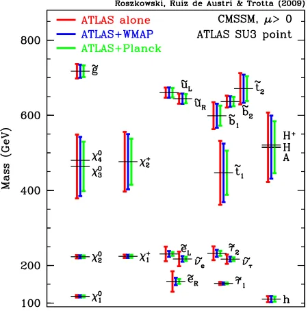
In Fig. 7 we show the constraints on the masses of several superpartners obtainable with the three sets of data considered in this paper. We can see that in the case of the gauginos (χ0

1,2, χ±1

and eg), whose masses are determined primarily by m1/2 (which is well reconstructed), the errors

are rather small, while for higgsino-like states (χ0₃_,₄ and χ±₂) the errors are large because of a poor determination of the µ parameter. For the states whose mass strongly depends on m0 (spin-zero

superpartners) the errors again reflect that of the common scalar mass, whose reconstruction, while reasonable, is not as good as for m₁_/₂.

The impact of further imposing other often used constraints from b→sγ and (g−2)µ is in the

present case rather limited. This is because the total error in the first quantity is still substantial while the dominant SUSY contribution to (g −2)µ comes from sneutrino-chargino exchange. In

the low mass region the masses of both particles are low and thus their contribution can be large enough to significantly reduce the discrepancy between the experimental data and the SM value.

Finally, we investigate how well one can predict the spin-independent cross section σSI

p of dark

matter neutralino scattering off a proton tested in direct detection experiments. As can be seen from Fig. 8, at 68% the value of σSI_p will remain uncertain to within about one order of magnitude, while the neutralino mass will be very well constrained by LHC data as a reflection of the bounds on

m1/2. This is because in the case studied here σpSI is too a large extent determined by a t-channel

heavy scalar Higgs exchange, where, in addition tomχ, the main two parameters are tanβ and the

Higgs mass which shows a considerable spread of values, mostly due to the larger uncertainty in

m0. Adding information about the DM relic abundance therefore improves the situation only in a

(17)

m

1/2 (GeV)

m 0

(GeV)

68%, 95% contours Black: ATLAS only

Blue: ATLAS+WMAP

true value

280 300 320

50 100 150 200 250 300 A

0 (TeV)

tan

β

68%, 95% contours Black: ATLAS alone

Blue: ATLAS+WMAP

true value

−2 0 2

10 20 30 40 50 60 m

1/2 (GeV)

m 0

(GeV)

Blue: ATLAS+Planck

true value

Posterior pdf

Log priors CMSSM, µ>0 ATLAS SU3 point

280 300 320

50 100 150 200 250 300 A

0 (TeV)

tan

β

68%, 95% contours Black: ATLAS alone

Blue: ATLAS+Planck

true value

Posterior pdf

Log priors CMSSM, µ>0 ATLAS SU3 point

−2 0 2

[image:17.612.80.511.107.549.2]

10 20 30 40 50 60

Figure 6: Impact of adding to the ATLAS data cosmological dark matter abundance determination with WMAP-like (upper row) and Planck-like (lower row) errors on (m1/2, m0) (left panels) and

(tanβ, A0) (right panels). Filled regions are for ATLAS plus either WMAP or Planck, while empty

(18)

[image:18.612.182.407.100.327.2]

Figure 7: Reconstruction of the SUSY mass spectrum using projected ATLAS data only (red/leftmost errobar), adding WMAP-like constraints on the dark matter relic abundance (blue/central errorbar) and adding Planck-like dark matter constraints (green/rightmost errorbar). The errorbars represent the 68% range of the Bayesian posterior for the log prior. (The results for the flat prior is essentially identical.)

3.4 Impact of a naturalness prior

We now turn to investigating the impact that a highly informative prior choice based on naturalness considerations would have on the Bayesian posterior. The CCR effective prior implements Occam’s razor penalization of regions of the parameter space exhibiting large fine-tunings [20]. This implies that the statistical weight of regions with large tanβ is reduced, since fine-tuning generally increases with increasing tanβ. The same applies to the soft-terms, except form0 where lower fine-tuning is

actually achieved in the TeV range, in the so-called hyperbolic branch/focus point (FP) region [26, 27].

The posterior pdf for the CCR prior for the CMSSM parameters is shown in Fig. 9 as blue-shaded 68% (darker) and 95% (lighter) regions, where for comparison we also show the non-informative log prior case (the corresponding black contours). We observe that the CCR prior leads to much tighter errors on especially tanβ, and to some extent also m0, by assigning a larger penalty, and

therefore stronger constraints, to “less natural” ranges of those parameters. The posteriors for

m1/2 and A0, on the other hand, are only midly affected by the CCR prior. This is an example

(19)

m

χ (GeV)

log(

σ p

SI ) (pb)

Blue: ATLAS+WMAP

true value

110 115 120 125

−9.5 −9 −8.5 −8 −7.5 −7 −6.5

m

χ (GeV)

log(

σ p

SI ) (pb)

Blue: ATLAS+Planck

true value

110 115 120 125

[image:19.612.75.510.109.317.2]

−9.5 −9 −8.5 −8 −7.5 −7 −6.5

Figure 8: Impact of adding to the ATLAS data cosmological dark matter abundance determination with WMAP-like (left panel) and Planck-like (right panel) errors on the predictions for the spin-independent cross section of dark matter neutralino scattering off a proton, relevant for direct detection experiments. Filled regions are for ATLAS plus either WMAP or Planck, while empty contours are for ATLAS only.

4 Comparison with profile likelihood

In order to examine the robustness of the results obtained with the Bayesian posterior pdf, in this Section we compare them with what would be obtained by using a more traditional χ2_-based

analysis. We thus define theprofile likelihoodfor, e.g., the CMSSM parameterm1, wherem1, . . . , m8

comprise the 4 CMSSM parameters and the 4 SM nuisance parameters of Table 1, as

L₍_m₁₎_≡ _max

m2,...,m8L(d|m), (7)

(20)

m

1/2 (GeV)

m 0

(GeV)

68%, 95% contours Black: ATLAS (Log prior)

Blue: ATLAS+naturalness prior

true value

Posterior pdf CMSSM, µ>0 ATLAS SU3 point

280 300 320

50 100 150 200 250 300

A

0 (TeV)

tan

β

68%, 95% contours Black: ATLAS (Log prior)

Blue: ATLAS+naturalness prior

true value

Posterior pdf CMSSM, µ>0 ATLAS SU3 point

−2 0 2

[image:20.612.82.510.109.317.2]

10 20 30 40 50 60

Figure 9: 2D posterior pdf for the case of applying ATLAS mass spectrum data alone with an informative naturalness prior (the CCR prior, filled contours), compared with the posterior obtained using non-informative log priors (empty contours).

are dealing with simulated data and we can thus double check that our profile likelihood correctly peaks near the true maximum likelihood value. Since we have found above little prior dependence of the posterior pdf, this suggests that the posterior pdf is dominated by the likelihood. Therefore we generically expect that the profile likelihood will give similar statistical results as the posterior studied above.

This is indeed confirmed in the top row of Fig. 10, where we present the 68% (inner contours) and the 95% confidence regions (outer contours) of the profile likelihood for the ATLAS-only data case and we compare them with the analogous regions derived from the posterior pdf presented earlier in Fig. 1. We show only the log prior case as the profile likelihood is prior independent (which we have verified numerically). We can see that at the 95% CL from the profile likelihood is quite similar to the corresponding 95% region derived from the Bayesian posterior for all parameters, except for m0, for which the profile likelihood yields looser constraint. It is worth noticing that

the posterior pdf yields a somewhat better reconstruction of m0 and tanβ and a similar one for

the other CMSSM parameters. However, the relative merits of the reconstructed confidence regions from the posterior or from the profile likelihood cannot be assessed here. It is in general a difficult task to decide which statistics yields the “best” results (however one chooses to define this). A possible way forward would be to carry out a coverage study of the quoted confidence intervals, which is beyond the scope of this paper.

(21)

m

1/2 (GeV)

m 0

(GeV)

68%, 95% contours Black: ATLAS, posterior pdf

Beige: ATLAS, profile likelihood

true value

280 300 320

50 100 150 200 250 300

A

0 (TeV)

tan

β

68%, 95% contours Black: ATLAS, posterior pdf

Beige: ATLAS, profile likelihood

true value

−2 0 2

10 20 30 40 50 60

m

1/2 (GeV)

m 0

(GeV)

68%, 95% contours Black: ATLAS+Planck, posterior pdf

Beige: ATLAS+Planck, profile likelihood

true value

280 300 320

50 100 150 200 250 300

A

0 (TeV)

tan

β

68%, 95% contours Black: ATLAS+Planck, posterior pdf

Beige: ATLAS+Planck, profile likelihood

true value

−2 0 2

[image:21.612.75.510.91.541.2]

10 20 30 40 50 60

Figure 10: Comparison between the profile likelihood (filled) and posterior (empty contours) using ATLAS mass spectrum data only (top row) and adding Planck (bottom row). With this combination of data, the choice of statistics (Bayesian posterior or profile likelihood) becomes almost irrelevant, giving intervals that match at the 10% level.

(22)

Fig. 10 for the ATLAS+Planck case, which should be compared with the bottom row of Fig. 6.

5 Summary and conclusions

In this paper we have examined prospects for reconstructing supersymmetric parameters from as-sumed future data that one can reasonably expect to become available. To this end we focused on the Constrained MSSM and on the benchmark point ATLAS SU3.

By following the ATLAS assumptions as closely as possible without having access to the full simulated likelihood function, we arrived at generally rather similar results for the reconstruction of the CMSSM parameters, with the exception of A0, for which our projected limit appears

some-what weaker. We stress here that our method is generally applicable, and that the quantitative discrepancies observed with the ATLAS collaboration result are a consequence of the limited in-formation available about the precise shape of the likelihood function. We therefore would urge experimentalists to make publicly available numerical fits to the likelihood functions that could be used to improved on the Gaussian assuption adopted here. We highlighted the computational advantage of our method which employs an effective likelihood at the mass spectrum level, which allows to shortcut the computationally expensive simulation of the whole experimental setup. We also demonstrated that, once LHC data become available, previously observed prior dependence of the results disappears if one adopts the broad, non-informative flat or log priors, although this may not be the case with any choice of this class of priors. We showed that the conclusions depend only mildly on which statistical quantity one chooses to adopt, i.e., Bayesian posterior or profile likelihood, in marked contrast with the present-day situation. The information from the likelihood can also be supplemented by a prior encoding a preference for “naturalness”, thus suppressing the statistical weight of finely tuned regions. This choice leads to tighter errors onm0 and tanβ, while

hardly affecting the conclusions on A0 and m1/2. We then extended the analysis by adding to

the likelihood function information about the neutralino dark matter relic abundance by imposing WMAP-like and Planck-like constraints. This improved the ability to reconstruct the value of es-pecially m0 and tanβ, much less so form1/2 (compared to the ATLAS data only case), while the

bi-modality in the determination ofA0 could not be removed.

(23)

Acknowledgements

The authors would like to thank D. Costanzo, R. Cousins, L. Lyons and D. Tovey for useful con-versations, as well as C. Topfel and M. Weber for providing the covariance matrix used in the ATLAS Collaboration Report [9]. A communication with K. Desch, M. Uhlenbrock and P. Wiene-mann is also acknowledged. We would like to thank an anonymous referee for useful comments. L.R. is partially supported by STFC, the EC 6th Framework Programmes MRTN-CT-2004-503369 and MRTN-CT-2006-035505. The work of R.R. is supported in part by MEC (Spain) under grant FPA2007-60323, by Generalitat Valenciana under grant PROMETEO/2008/069 and by the Spanish Consolider-Ingenio 2010 Programme CPAN (CSD2007-00042). L.R. would like to thank the CERN Theory Division for hospitality during the final stages of the project. R.T. would like to thank the Galileo Galilei Institute for Theoretical Physics for the hospitality and the INFN and the EU FP6 Marie Curie Research and Training Network “UniverseNet” (MRTN-CT-2006-035863) for partial support.

References

[1] G. L. Kane, C. F. Kolda, L. Roszkowski and J. D. Wells, Phys. Rev. D49 (1994) 6173 [hep-ph/9312272].

[2] A. Chamseddine, R. Arnowitt and P. Nath, Phys. Rev. Lett.49(1982) 970;R. Barbieri, S. Fer-rara and C. Savoy, Phys. Lett.B119 (1982) 343;L. J. Hall, J. Lykken and S. Weinberg, Phys. Rev.D27 (1983) 2359; for a review, see, e.g., H. P. Nilles,Phys. Rept. 110 (1984) 1.

[3] B. C. Allanach and C. G. Lester, Phys. Rev. D73 (2006) 015013 [hep-ph/0507283]; B. C. Al-lanach, C. G. Lester and A. M. Weber, JHEP 0612 (2006) 065 [hep-ph/0609295]; B. C. Al-lanach, Phys. Lett.B635 (2006) 123 [hep-ph/0601089].

[4] R. Ruiz de Austri, R. Trotta and L. Roszkowski, JHEP 0605 (2006) 002 [hep-ph/0602028]; L. Roszkowski, R. Ruiz de Austri and R. Trotta,JHEP0704 (2007) 084 [hep-ph/0611173] and

JHEP0707 (2007) 075 [arXiv:0705.2012].

[5] J. R. Ellis, et al., JHEP0605 (2006) 005 [hep-ph/0602220]. [6] O. Buchmueller et al., arXiv:0808.4128 [hep-ph].

[7] N. Arkani-Hamed, et al.,JHEP 0608 (2006) 070 [arXiv:hep-ph/0512190].

[8] I. Hinchliffe, et al.,Phys. Rev.D55(1997) 5520 [hep-ph/9610544]; C. G. Lester and D. J. Sum-mers, Phys. Lett. B463 (1999) 99 [hep-ph/9906349]; W. S. Cho, et al., Phys. Rev. Lett. 100

(2008) 171801 [arXiv:0709.0288]; G. G. Ross and M. Serna, Phys. Lett. B665 (2008) 212 [arXiv:0712.0943]; M. M. Nojiri, et al.,JHEP0805(2008) 014 [arXiv:0712.2718]; H. C. Cheng, et al.,JHEP0712 (2007) 076 [arXiv:0707.0030].

[9] G. Aad, et al., [The ATLAS Collaboration], arXiv:0901.0512.

[10] B. C. Allanach, Comp. Phys. Comm. 143(2002) 305 [hep-ph/0104145].

[11] G. Belanger, et al., Comp. Phys. Comm. 149 (2002) 103 [hep-ph/0112278]; MicrOMEGAs:

(24)

[12] J. Dunkley et al. [The WMAP Collaboration], Astrophys. J. Suppl. 180 (2009) 306 [arXiv:0803.0586].

[13] M. M. Nojiri,et al.,JHEP 0603 (2006) 063 [hep-ph/0512204]. [14] The Planck Collaboration, astro-ph/0604069.

[15] B. C. Allanach, et al., G. Belanger, F. Boudjema, A. Pukhov and W. Porod, hep-ph/0402161. [16] F. Feroz and M. P. Hobson Mon. Not. Roy. Astron. Soc. 384 (2008) 449; F. Feroz, et al.,

arXiv:0809.3437.

[17] B. C. Allanach, et al., JHEP 08(2007) 023 [arXiv:0705.0487]. [18] R. Trotta, et al., JHEP0812 (2008) 024 [arXiv:0809.3792].

[19] Y. Akrami, et al., JHEP1004 (2010) 057 [arXiv:0910.3950 [hep-ph]].

[20] M. E. Cabrera, J. A. Casas and R. R. de Austri,JHEP 0903 (2009) 075 [arXiv:0812.0536]. [21] M. E. Cabrera, A. Casas and R. R. de Austri, JHEP 1005 (2010) 043 [arXiv:0911.4686

[hep-ph]].

[22] J. R. Ellis, K. Enqvist, D. V. Nanopoulos and F. Zwirner, Mod. Phys. Lett. A1 (1986) 57. [23] R. Barbieri and G. F. Giudice, Nucl. Phys. B306 (1988) 63.

[24] See: http://www.superbayes.org/

[25] E. A. Baltz, et al.,Phys. Rev. D74 (2006) 103521 [hep-ph/0602187].

[26] K. L. Chan, U. Chattopadhyay and P. Nath, Naturalness, weak scale supersymmetry and the

prospect for the observation of supersymmetry at the Tevatron and at the LHC,Phys. Rev.D58

(1998) 096004 [hep-ph9710473 ].

[27] J. L. Feng, K. T. Matchev and T. Moroi, Multi - TeV scalars are natural in minimal

super-gravity,Phys. Rev. Lett. 84(2000) 2322 [hep-ph9908309 ] andFocus points and naturalness in