Maximum likelihood estimation of variance components

MAXIMUM

LIKELIHOOD

ESTIMATION

OF

VARIANCE

COMPONENTS

A thesis submitted for the degree of

Master of Statistics

of the Australian National University

November 1991

I, Alice Richardson, declare that all work in this thesis is my own.

ACKNOWLEDGEMENTS

I would like to thank my supervisor, Dr. Alan Welsh, for his helpful comments

throughout both the research and writing stages of this thesis. Thanks also to Ms.

Michelle Ross who provided help with Macintosh word processing, and to Professor

Charles Heathcote for his general support. Finally, thanks are due to my hall of

residence, Ursula College, where the in-college computing facilities are second to

ABSTRACT

In this thesis, the Maximum Likelihood and Restricted Maximum Likelihood methods

of estimating variance components are investigated for the one-way model.

Expressions for the estimators and their variances are obtained, and algorithms for

finding the estimates are tested by means of a Monte Carlo study. The quantitative

effects of non-normality on the variability of estimates are discussed. Finally,

diagnostic tests for identifying outliers and non-normality are proposed, and illustrated

CONTENTS

Statement of Originality i

Acknowledgements ii

Abstract iii

Contents iv

Introduction 1

ML and RE ML Estimation of Variance Components 6

Numerical Procedures for ML Estimation 13

Measures of Efficiency 19

Monte Carlo Study 26

Non-Normality 33

Diagnostic Tests 40

Conclusion 52

Mathematical and Statistical Results used in Variance Components Analysis 53

Splus Functions 60

1. INTRODUCTION

The complex covariance structure of the variance components model can be used to describe data arising in fields as diverse as designed experiments in agriculture and observational studies in the social sciences. This combination of complexity and wide applicability has meant that the estimation of variance components has been a rich source of research problems over the last century. Even so, there still remain unsolved problems pertaining to various facets of the variance components model, in particular, which estimation method is to be preferred in a particular situation. Many kinds of estimator have been proposed, with very few guidelines for choosing between them.

The objective of this thesis is to investigate the classical methods of estimating variance components, concentrating on Maximum Likelihood (ML) and Restricted Maximum Likelihood (REML) for the one-way mixed model, in both the balanced and unbalanced case.

1.1 DESCRIPTION OF THE MODEL

Consider the general linear model:

c

y = Xa + X Z j ß j + e (1.1)

i=l

where y is a n-vector of observations, X and Z\ are known n x q and n x pj design matrices respectively; a is a q-vector of fixed effects; the ßi are pj-vectors of random effects, 1 < i < c; and e is an n-vector of errors. The pi levels of each random effect are assumed to be a random sample from an infinite population of levels. By putting Var(ßi) = Di and Var(e) = R, we obtain

c

Var(y) = R + X Z A Z jT = V. i=l

The problem is to estimate R and D i , . . . , Dc.

The standard variance components model is a special case of (1.1). Often a reduces to a single parameter, the overall mean, which will be the situation throughout this thesis. The levels of each factor ßi are assumed to be independently normally distributed with

2

mean zero and variance a -. Similarly, each random error is assumed to be

2 2

independently normally distributed with mean zero, and variance Gq = G £. Finally, ßi

and e are assumed to be uncorrelated.Thus Di = o | Ipi where Ik is a k x k identity 2

matrix, R = o £In, and

2

c c

i=l i=l

2 2

where Gi = 7j{Z\ . The problem reduces to estimating g£ and Gj,

i=l

2 2

1, . . . , G c.

Some authors use a slightly different parameterisation in terms of y:

2 2 2

Yi = G j / o e, i = 1, . . . , c and w = a e.

The G2 formulation is used in this thesis because it is usually easier to work with the actual parameters requiring estimation. It is however a simple matter to move between parameterisations using the Jacobian of the transformation.

According to Rao and Kleffe (1988), the first use of variance components was in the work of astronomers Airy (1861) and Chauvenet (1863), who used a one-way random model. Fisher (1918) was the first to use the term “analysis of variance” (ANOVA) and Eisenhart (1947) introduced the term “Model II” for the random (or mixed) effects model that lends itself to variance component analysis.

But it is Henderson’s (1953) paper that could best be described as the “landmark” piece of research in this field, for Henderson cites only four earlier papers, but most subsequent researchers cite him. (Those four earlier papers are Crump (1946, 1951), Eisenhart (1947) and Hazel and Terril (1945).) Essentially all the papers before Henderson dealt with specific cases: Henderson was the first to present methods in general. Henderson proposed three methods of estimating variance components: they are all variations on ANOVA estimates which involve equating various quadratic forms of the observations to their expected values, then solving for the variance components. His methods are still popular as a first attempt at estimating variance components.

Other methods involving equating quadratic forms to their expectations have since been proposed e.g. symmetric sums estimators. Searle’s (1981) book contain lists of formulae for this particular method for models with up to three crossed factors.

there exists a wide variety of ANOVA methods, but no clear criteria for choosing between them.

Hartley and Rao (1967) took a step away from this confusing situation when they developed a procedure for the maximum-likelihood estimation of components of variance based on the steepest-ascent method of solving equations. They also discussed asymptotic efficiency of the estimates by looking at the second derivative of the log likelihood. Searle (1970) also derived formulae for variance matrices in the same way.

However ML estimates (MLEs) are not perfect either - their main drawback is bias. The simplest example of this is also a very well-known one - that of estimating the single “variance component” a 2 of a N(q, o2) distribution, when fi is unknown. If a random sample x i , . . . , xn is taken from the distribution, the MLE of o2 is

r 2 > i - x ) 2

which has expected value The unbiased estimator, which effectively takes into

account the fact that the mean is unknown and must be estimated too, is therefore (xi - x)2 .

Patterson and Thompson (1971) incorporated this notion of allowing for the estimation of fixed effects by maximising the likelihood, not of all the data, but of a selected set of "error contrasts". (An error contrast is defined as a linear function S of y whose expectation is 0.) Letting Var(y) = V, the set of error contrasts they chose has a singular covariance matrix, STVS, even though the inverse of this matrix is required in the derivative of the likelihood. Patterson and Thompson overcame the difficulty by substituting the spectral form of s V s into the likelihood, however the variances to be estimated are then embedded in the eigenvalues, so differentiating with respect to them is still awkward.

Corbeil and Searle (1976a) avoided the singularity issue by taking the error contrasts to be a set of (n - rank(X)) rows of S, and they called their new estimators REML estimators. In their paper they cover estimation by a version of the Newton-Raphson method and the variance matrix of the estimates. The same authors (1976b) also compare the variance of ML and REML estimators for balanced designs up to two- way, and give a numerical example of an unbalanced two-way crossed model without interaction.

More recently, authors such as Fellner (1986) and Hocking, Green and Bremer (1989) have been addressing the problem of estimation for non-normal data, and diagnostic tests to detect non-normality. Non-normality is a problem with real-life data, and it can occur in many ways because of the complex nature of experiments analysed by variance components, often involving several crossed or nested factors. There appear to be two basic approaches to non-normality as represented by these two papers:

1) derive new estimators that also identify outlying observations (Hocking et al.)

2) robustify current estimators to reduce the effect of outlying observations on the estimate (Fellner).

Parallelling this series of estimators was the development of MINQEs and MIVQUEs. MIVQUES are Minimum Variance translation-invariant Quadratic Unbiased Estimators. In this context, the quadratic form yTAy is translation-invariant if (y - Xa)TA(y - Xa) = yTAy i.e. AX = 0. For the standard variance components model following (1.1),

c

where ßi ~ N(0, G^IpO and e - N(0, GqIo), the MIVQUE of ^ V iG ^ is yTAy, where A i=0

c

is chosen to minimise Var(yTAy), subject to E(yTAy) = The main drawback of i=0

the procedure is that it sometimes produces negative estimates of variance.

Minimum Norm Quadratic Estimators are a whole family of estimators: MINQUEs (Unbiased), MINQIEs (Invariant), MINQUIEs (Unbiased and Invariant), MINQUNNDEs (Unbiased and Non-Negative Definite) and MINQENNDEs (Invariant and Non-Negative Definite). Briefly, the derivation of MINQEs is as follows (see Rao and Kleffe (1988)):

A natural estimator of ^ \ [ G | 2is ßTLß (for some suitable L.) We estimate ßTLß by i=0

t. R . ( X TA X X TA Z U a

y Ay - ( o ß ) ( ZTAX ZTAZ j (ß

The aim is to minimise the difference between L and A i.e. minimise

— _

X AX X AZ

Harville (1977) states that MIVQUE assuming normality is equivalent to MINQUE assuming || || is the Euclidean norm. Under these conditions also MIVQUE (that is, MINQUE) is equivalent to the first iteration of REML. Rao and Kleffe (1988) also state that MINQE is equivalent to the first iteration of ML. Thus MINQE and MIVQUE are contained within ML and REML estimation respectively.

These last two techniques, ML and REML, are the focus of this thesis.

2. ML AND RE ML ESTIMATION OF VARIANCE COMPONENTS FOR THE ONE-W AY MODEL

2.1 AN EXAMPLE OF A ONE-W AY EXPERIMENT

Several of the published articles about variance components include data sets to illustrate the points being made. The data set used to illustrate this thesis, given in Table 2.1, is quoted by Hocking (1985) and comes from Snedecor and Cochran (1967). They explain that the data are from “ an experiment in which four seed treatments were compared with no treatment (Check) on soybean seeds. The data are the number of plants which failed to emerge out of 100 in each plot.”

Table 2.1. Number of soybean plants (out of 100) failing to germinate treatment____________________ replications

Check 8 10 12 13 11

Arasan 2 6 7 11 5

Spergon 4 10 9 8 10 Semesan Jr 3 5 9 10 6

Fermate 9 7 5 5 3

2.2 THE GENERAL O N E-W A Y MODEL

The soybean experiment in Table 2.1 can be expressed in general terms as follows: Total

Treatment 1 _{y n • yim} Ti

Treatment p _{ypi • ypnP Tp}

Total G

or in matrix notation as y = X a + Zß + e

A n \ A \

Am

A

( ß l 1

where l ni is a njxl vector of ones. If the experiment is balanced, there are the same number of observations in each treatment i.e. nj = m for 1 < i < p. Otherwise, the experiment is unbalanced. In terms of the model (1.1), c = 1 and p denotes the number of levels of ß.

2 2 2

To simplify notation, let o £ = e and Gj = Gß = b. Therefore

Var (y) = V = R + ZDZT

\

= eln + b *

Jnp

)

where Jm is a m x m matrix of ones

ZZT.

The matrix V is non-zero only in blocks down the diagonal, and we may thus refer to the ith diagonal block of V as elni+ bJni , i = 1, . . . , p.Then using the fact that

(eIni+ b J ni)-'= “ Ini- (e(e+nib)) Jm (Graybill (1983) p. 190),

V 1 is block diagonal with blocks of

f

e(e+nib) e(e+nib)

-b e+(nj-l)b

\e(e+nib) e(e+nib)

J

The block diagonal structure of V and V-1 greatly simplifies the calculation of the likelihood in the one-way case, because it carries through to most of the matrices involved. The expression “ith block” next to a matrix means that the matrix is block diagonal, and that only the ith block has been written down.

2.3 ESTIMATION OF EFFECTS

Even though the effects ß and e are not parameters, it is useful to estimate them because they can in turn be used to estimate the parameters of interest, the variance components. An estimate of the parameter a is required for the same reason.

The MLE of a is easily shown to be a = (XTV"1X)"1XTV“1y. For the one-way model

a = (1 . . . 1)

f e+ (n j-l)b - b e(e+nib) e(e+nib)

\

- b e+ (n j-l)b

1

\e(e+ nib) e(e+nib) / Vyini

J

Itv-lü

ij

ith block

^ e + n ib ^ ^ e + n j b (2'2)

i=l i=l

which reduces to the overall mean y if the experiment is balanced.

No MLE of ß exists because ß does not feature in the likelihood. The best (minimum MSE) predictor of ß, derived in the Appendix at (A 1.1), is ß = DZTV_1(y - Xd), and it follows immediately that the best predictor of e is e = y - X d - Zß. The expression for ß in the one-w ay model is

f

( b b '\

e+nib ' * e+nib

v

f

^ b ( y i ~ a )

e+npb ‘ * e+npb )

\Ypnp a /

npb

^ ( y P - a)

(2.3)

J

\e+ n p b v = D ZTPy

where P = V "X (X TV 'X ) _1X TV "

= V

-I e + njb r l

^ ___!___ j (e+nib)2 nl

1

A

\ s(e+nib)(e+njb) njxm where Jnixnj is a n* x nj matrix of ones.

Therefore P has diagonal blocks of

(e+nib)(e+njb)

(e+npb)2Jnp

•nixnj

^(e+nib)(e+(ni-l)b)(Eni/e+nib) - e

e(e+nib)2(Zni/e+nib)

-b(e+nib)(Zni/e+njb) - e

^ e(e+nib)2(Zni/e+nib)

-b(e+nib)(Zni/e+nib) - e '

e(e+nib)2(Zni/e+nib)

(e+nib)(e+(ni-l)b)(Zni/e+nib) - e

e(e+riib)2(Enj/e+nib)

J

and off-diagonal blocks o f -1

>nixnj-(e+nib)(e+n;b)(Zni/e+nib)

The matrix P w ill be seen in the next section to be a very important quantity in REML

estimation, because it is the inverted variance matrix with a correction allowing for the

fact that a has been estimated. The expression e + njb that is a feature o f the elements

o f P in the specific context o f the one-way model w ill also be seen again and again.

2.4 ESTIM ATIO N OF V A R IA N C E COMPONENTS

2.4.1 M A X IM U M LIK E LIH O O D

To estimate e and b, we start with the log likelihood, L. Ignoring terms free o f e and b

L = (-1 /2 ) log[|V |] - (1/2) (y - X a )TV "(y - X a ). (2.4)

Using (A1.5) to differentiate (2.4) with respect to e

3L/3e = (-1 /2 ) tr[V~‘(3V/3e)] + (1/2) (y - X a )TV~'(3V/3e)V''(y - X a )

= (-1 /2 ) tr[V "] + (1/2) (y - X & )TV “ V "(y - X a ) replacing a by cc, and

noting that 3V/3e = I n.

= (-1 /2 ) tr

f

e(e+nib) e(e+nib)

- b e + (n i-l)b

\e(e+nib) e(e+nib)

_J

ith block

f (e+C nj-Q b^O ii-Q b2

e2(e+nib)2

- (y u -a , . . .,yini-a)

-2 b e-n jb 2 \ e 2(e+nib)2

-2 b e -n jb 2 e2(e+nib)2

A

/'yu -a A

(e + (n j-1 )b)2+ ( n j- 1 )b2

e2(e+njb)2

J

- )

ith block

= * 9L/3e = ~ l t

I V _> _ L V YrlV nKyj-g)2

2 2mU e+nib 2e2 ~ ^ ^ 2j2 L (e+nib)2

i=l 1=1 J=1 i=l

(2.5)

Similarly, differentiating (2.4) with respect to b,

dL/db = (-1/2) tr[V-1(öV/3b)] + (1/2) (y - X a)TV'1(0V/9b)V1(y - Xa) and after replacing a by a and recalling that 8V/3b = ZZT = G,

8L/öb = (-1/2) tr[V_1G] + (1/2) (y - X a)TV '1G V 1(y -X a)

/ i i \

e+njb ' ‘ e+njb

= (-1/2) tr ith block

1 1

ye+nib ' * e+njb J

+ ( y i i - a , • • yim -a )

f ni_{e+nib ’ e+njb}ni A

ni ni

\e+ njb ‘ e+njb J

/V i l - a A

ith block

Vyini-a )

ni 1 X"1 nj2(yj - a )2

2 Zm4 e+njb 2 ZmJ (e+njb)2

i=l i=l

(2.6)

2.4.2 RESTRICTED MAXIMUM LIKELIHOOD

Now the likelihood equation for finding the REML estimates differs from (2.4) by only one term, as below:

Li = (-1/2) log[|V|] - (1/2) log[|XTV-1X|] - (1/2) (y - X a)TV-1(y - Xa) (2.7) so that the derivatives are (using (A 1.6)):

3Li/8e = (-1/2) tr[P] + (1/2) (y - X a )JW~lW~\y - Xa) P

-1 \ 1 nj(e+nib)(e+(nj-l)b)(Zni/e+nib) - nje

2 e(e+nib)2(Zni/e+nib)

3Li/3b = (-1/2) tr[PG] + (1/2) (y - Xöc)TV 1GV'1(y -X a)

= (-1/2) tr

(

________ ZOJ_________

\^(e+nib)(e+njb)(Xni/e+nib) >njxni

---—--- J

(e+nib)(e+njb)(Xni/e+nib) m*nj

(e+npb)(Znp/e+npb) - np

(e+npb)2(Lnp/e+npb) np

J

+ (1/2) (y - X a)TV"1GV"1(y -X a)

P P

3l Y f(e-t-njb)(Znj/e+njb) - ni A 1 Y ni2(Yi ~ ä )2

2 1 (e+nib)2(Zni/e+nib) J 2 2 m J (e+nib)2

i=l i=1

(2.9)

2.5 A SPECIAL CASE OF EXPLICIT SOLUTIONS

If the experiment is balanced and the ANOVA estimates are positive, then (2.8) and (2.9) can be used to show that REMLEs are equivalent to ANOVA estimates, as follows. The ANOVA table for a one-way balanced experiment is

source of error dof SS MS E(MS)

treatments p-1 m l(yi - y)2 SS /p-l = MSB e + mb

error n-p II(y ij - yO2 SS/n-p = MSE e

total n-1 ZZ(yij - y)2

and equating mean squares to expected mean squares we obtain the ANOVA estimates ~ M S B -M SE

of the variance components: e = MSE and b = --- .

Writing (2.9) for balanced data:

\ T „ -(n - m) m SSB

5Li/3b = 0 =» — r r +

2(e + mb) 2(e + mb)2

SSB

0

=>

—

p-1

and (2.8) can be written

, -n(e + (m-l)b) + e SSE SSB

3L/5e = 0 => _ 28(8 + mb) + 2(8+"mb)2 = 0

-mn(e + (m-l)b) + me SSE e(n - m) . -me(e + mb) + e2 + me(e + mb) _ usin§ SSE

=> e = --- = MSE, the ANOVA estimate of e. n - p

Substituting back in (2.10), b = ---, the ANOVA estimate of b.

Similarly, explicit MLEs can be calculated if the data is balanced. Writing (2.6) for balanced data yields

-nt /-\i -n mSSB

OL/Ob = 0 => — — +

2(6 + mb) 2(e + mb)2 0 => e + mb

SSB

(2.11)

while (2.5) for balanced data reads

-nt A n - p p SSE SSB

^ e ~ ^ -2 e 2(e + mb) + 2e2 + 2(e + mb)2 ~

n - P SSE

=> e

e e + mb SSE

+ e2 + e + mb

n - p = MSE.

Substituting back in (2.11), b (SSB/p) - MSE

using (2.11)

These exact results will be used to calculate measures of efficiency in the balanced case (Chapter 4).

2.6 DISCUSSION

3. NUMERICAL PROCEDURES FOR MAXIMUM LIKELIHOOD ESTIMATION

This chapter examines two procedures for obtaining MLEs and REMLEs by iteration. They are not the only methods by any means, but their advantages are

1) they are both conceptually clear

2) they both lend themselves to be written in the form of Splus functions 3) they have not been thoroughly investigated in the published literature.

3.1 ANDERSON’S ALGORITHM

Differentiating the likelihood (2.4) with respect to 0i (where 0i, i = 1, 2 are the elements of the vector of parameters 0 = (e, b)T) and setting the result equal to zero we obtain

3L/a0i = 0 =* tr[V_1(av/a0i)] = (y - Xa)TV'1(av/a0i) V 1(y - Xa).

The left hand side can be rewritten as

tr[vl(av/a0i)] = tr[v_

1

(av/a0i)] z v^av/aopOj

= z tr[v"

1

(av/a0i)v"

1

(av/a0j)] Oj

= tr [v 1(a v /a 0 i)v 1(av/a0j)] 0

so that

tr[v“1(av/a0i) v 1(av/a0j)] 0 = (y - x a ) Tv"l(av/30i)v~l(y - x a ) B0 = d

0 = B"‘d. (3.1)

If we start with (2.7), the restricted maximum likelihood Li, the algebra is very similar.

aLi/00 = 0 => tr[P(av/a©i)] = (y - Xa)TV 1(av/a0i)V"1(y - Xa) But the left hand side equals tr[P(0V/00i)P(0V/30j)] 0 so that tr[P(3V/30i)P(3V/30j)] 0 = (y - Xa)TV'1(av/a0i) V 1(y - Xa)

Bi0 = d

0 = B j'd (3.2)

where B, Bi and d depend on 0.

The matrix B

M V -2] tr[V G V ‘] v

U tV 'G V "1] tr[V'GV'G]

and for the one-way model the individual traces are as follows:

tr[V-2] = tr

f

-2 b e -n jb 2 Vve2(e+nib)2

-2 b e -n jb 2 e2(e+nib)2

A

(e+ (n j-l)b )2 + (n j-l)b 2 e2(e+nib)2

J

ith block

r

s

A /(e + m b )2 Jm

trtV'GV"1] = tr

\

V l/(e+ n pb)2 Jnp

j

I

i= l

tr[V_1G V_1G] = tr

(

V

A

np/(e+npb)2 Jnp

)

s

(e+nib)2

Similarly for REML, the matrix B i

/tr[P2] tr[PGP] ^ tr[PGP] tr[PGPG] and each trace is

tr[P2]

f

= tr

e(e+nib)2(Enj/e+nib)

-b(e+nib)(Enj/e+nib) - e y e(e+nib)2(Znj/e+nib)

(3.3)

(3.4)

(3.5)

A

e(e+nib)2(Zni/e+nib)

(e+njb)(e+(nj-l)b)(Lni/e+nib) - e e(e+nib)2(Zni/e+nib)

J

(ith diagonal block; offdiagonal blocks are -1

I

e(e+nib)2(Zn[/e+njb) i=l

+ (n ,-l)

n(e2+ 2 (m -l )eb+m (m -l )b2) e2(e+mb)2

f-b(e+nib)(Zni/e+nib) - e ")_{2 + V ___________ m___________ 1}

v e(e+nib)2(£ni/e+njb) y ^^((e+ n ib )(e+ n jb )(£ n j/e+ n ib ))2

if the experiment is balanced. (3.6)

tr[PGP]

f

_________ = 3__________ \^(e+nib)(e+njb)(Zni/e+nib) 'njxni

_________ ZOi__________J . (e+nib)(e+njb)(£ni/e+nib)

e(e+npb)(Znj/e+njb) - npe e(e+npb)2(Enj/e+nib) np

A

J

i=l

["(e(e+njb)(Zni/e+njb) - nje)((e+nib)(e+(ni-l)b)(Zni/e+njb) - e) 1|_ (e(e+nib)2(Znj/e+nib))2

(-b(e+njb)(Xnj/e+nib) - e)(e(e+nib)(Znj/e+nib) - n^e)

+ (n i-1 )

I

(e(e+nib)2(Znj/e+nib))2

njnj

((e+nib)(e+njb)(Zni/e+nib))2

n - m

(e+mb)2 for balanced data (3.7)

tr[PGPG]

f 2(e+nib)(Zni/e+nib) - nie

e(e+n i b)2(Zni/e+nib)

= tr

_________ zPj__________ \^(e+nib)(e+njb)(£ni/e+nib)

P

Jm ~ n i

(e+nib)(e+njb)(Zni/e+nib) nixnj

e(e+npb)(Znj/e+njb) - npe

njxn‘ e(e+npb)2(£ni/e+nib) p _J

I

r

v (e+njb)2(£ni/e+nib) y -f*

((e+nib)(e+njb)(Zni/e+nib))2

= ~ e'+mb)2 f°r balanced data. (3.8)

These traces show again how important the expression e + njb is to ML and REML estimation. Furthermore, they will be re-used in calculating measures of efficiency (Chapter 4).

Finally, for both ML and REML, the vector d comes from (2.8) and (2.9) and is made up of the two elements:

(y - X ä)TV-2(y - X&) = J_ e2

nj(yj - a)2

(e+njb)2

(y - X a)TV"1GV"1(y - Xa) nj2( y j - a)2 (e+njb)2

The iterative part of the algorithm consists of choosing starting values for e and b, substituting them into B or B] and d, and solving for the new values of e and b. The algorithm will always converge, because B and Bi are always positive semidefinite. The proof for B is given below:

For a matrix to be positive semidefinite, we require that 5tB8 > 0 for any vector 5.

Now

5tB5 = X [B]jk 5j Sk

X tr[v-'ov/aej)v-Iov/aek)] SjSk

j.k

= üjV1 X av/aej Sj v" £ 3v/aek sk j

=

I av/aej

which is non-negative unless V“1 ^ 3V/30J 8j = 0 which is impossible since V"1 is j

non-singular and the 3V/30j are linearly independent.

The proof for Bi cannot follow the same route because P, which replaces V"1 throughout the proof, is definitely singular! But “for fixed 0 with V nonsingular, Bi is positive semidefinite and the linear system Bi0 = d is consistent for 0 (LaMotte 1973, pp. 316 and 327-8). The matrix Bi is nonsingular if and only if 0j is estimable in the class of quadratic translation-invariant estimators for i = 1, . . . , m (again see LaMotte

3.2 HENDERSON’S ALGORITHM

The derivation of Henderson’s algorithm uses the lengthy manipulation of the log likelihood given in Lemmas A 1.5 - A 1.8. From Lemma A 1.7

e = yT(y - Xcc - Zß)/n (3.9)

and from Lemma A 1.6

3L/9Gj = (-1/2) tr[(I - (I + ZTR"‘ZD)',)DH(3D/39i)] + (l/2)ßTD''(3D/30i)D'‘ß. Recalling that 9 = (e, b)T, we can substitute b for 9j and obtain

3L/3b = (-1/2) (1/b) (p - tr[(I + ZTR '‘ZD)'']) + (l/2b2)ßTß = 0 at a stationary point

=> b = ßTß/(p - tr[(I + ZtR''ZD)'‘]). (3.10)

Similarly for REML estimation, Lemma A1.8 proves that

e = yT(y - Xct - Zß)/(n - 1) (3.11)

and Lemma A 1.6 proves that

3Li/30i = (-1/2) tr[(I - (I + ZTSZD)_1)D_1OD/a0i)] + (1/2) ßTD_1(ÖD/00i)D‘lß. Since 0 = (e, b)T:

3Li/0b = (-1/2) (1/b) (p - tr[(I + ZTSZD)-1]) + (l/2b2)ßTß = 0 at a stationary point

=> b = ßTß/(p - tr[(I+ ZtSZD)_1]). (3.12)

Expressions for a, ß, (1+ ZTR_1ZD) and (I + ZTSZD) in the one-way case can be found at (2.2), (2.3), Lemma A1.2 and §A1.5. They all depend on e and b. The iterative part of the algorithm consists of choosing starting values for e and b; substituting them in the right hand side of (3.9) and (3.10), or (3.11) and (3.12); thus obtaining the updated values of e and b.

3.3 ILLUSTRATION WITH REAL DATA

The soybean data used to illustrate these procedures is documented in §2.1, and Splus functions to calculate the MLEs and REMLEs are at (A2.5) - (A2.8). The estimates and number of iterations required to find them were:

method e b # iterations

Anderson ML 6.82 1.9896 2

Henderson ML 6.82 1.99 11

Anderson REML 6.82 2.828 2

Henderson REML 6.82 2.83 9

Anderson’s algorithm is to be preferred in this case because it converges more quickly. The REMLEs are equal to ANOVA estimates because the data set is balanced, and as such could be calculated in one iteration.

4. MEASURES OF EFFICIENCY 4.1 GENERAL THEORY

A first-order approximation to the variance of the MLE 0 of 0 is [E 0 2L/aeaeT)r'[E 0 L /9 e)0 L /ae)T][E 0 2L/aea0T) r \ which is found by expanding L = log f(y, 9) in a Taylor series around 9.

But -E(3L/30)(3L/30)t = E(32L/3030T) when the distribution of y truly is f since E(32L/3030t) = E(32logf/3030T)

= J -(i/f)2

0

0

= J-0 io g f/ae )0 io gf/ae)T f dy = -E0iogf/ae)(aiogf/ae)T

Thus the information matrix = F = -E(32L/3930T) and the variance matrix = F~\ The diagonal elements of F"1 are of course the variances of the individual estimates, and their value is a lower bound on the variance of any estimate of 0.

4.2 ONE-WAY VARIANCE COMPONENTS MODEL 4.2.1 MAXIMUM LIKELIHOOD

The general second derivatives of the ML equation,and their expected values are at (A 1.6). Letting 0 = (e,b)T, the elements of the information matrix F are:

E(32L/3e2) = -E(3L/3e)2 = (-1/2) tr[V '2]

E(32L/3e3b) = -E(3L/3e)(3L/3b) = (-1/2) trtV^GV"1] E(32L/3b2) = -E(3L/0b)2 = (1/2) trtVGV^G].

There is no need to evaluate information and variances for a because fixed effects are not the focus of this thesis, and the co-information between a and the variance components, -E(32L/3a30i) = 0 i.e. the information matrix including a is block diagonal and information about a does not affect information about the variance components.

For the one-way model, (3.3) - (3.5) are used to calculate each piece of information as follows:

P

. r l V feZ+Ifni-DebEniCni-Ub2',

info(e) = (1/2) tr[V 2] = - 2 ^ "i I e2(e+nib)2 J ( 4 1 ) i=l

co-info(e, b) = (1/2) trtV 'G V "1] 1

I;

(4.2)

info(b) = (1/2) tr [ V 'G V ‘G] =

i=l ni2 (e+nib)2

Thus the information matrix, F, is

( p

1 \ ' /e 2+ 2 (n j-l)eb + n i(n j-l)b 2\

_{i V}

p

_ni

^

J

i= l

2 jLu (e+nib)2 i=l

P 1

Y

P

1 Y ni2 2 (e+n[b)2

i=1

2 ^L^(e+njb)2 i=i ;

and its inverse, Var(9) = ( ~b) )

f 2e2(Z(nje/e+njb)2) - 2 e 2(Zni e2/(e+njb)2)

(4.3)

(4.4)

\

- 2 e 2(Znje2/ (e+nib)2) 2(e2+ 2 (n j-l)e b + n i(n j-l)b 2)

(4.5)

\n(Z (nje/e+nib)2) - (Znje/e+njb)2 n(Z(nie/e+njb)2) - (Znje/e+njb)2

J

f

Searle (1970) rewrites info(e) as ^

2 jd

(e+njb)2+ n - p

V

A

J

but this is equivalent to

(4.1) only if the data is balanced. If that is the case, the variance matrix of the variance components is

4.2.2 RESTRICTED MAXIMUM LIKELIHOOD

As given in (A 1.6), the elements of the information matrix are

-E(32L i/aeaeT) = (1/ 2) tr[P O v /ae)P 0 v /ae)T].

Using (3.6) - (3.8) to evaluate each piece of information:

2 info(e) = tr[P2]

P

\ ^ [((e+nib)(e+(ni-l)b)(Zni/e+nib) - e ^ 2

=

2

i=l

+ (ni-1)

n(e2+ 2 (m -l)eb + m (m -l)b 2) .

if the experiment is balanced /^-b(e+nib)(Zni/e+nib) - e ^

2 +

y

ni

1

^ e(e+nib)2(Zni/e+nib) ((e+nib)(e+njb)(Zni/ e+njb))2

j+i 2

(4.7)

2 co-info(e, b) = tr[PGP]

P

I

(—b(e+nib)(Zni/e+nib) - e)(e(e+nib)(Zni/e+nib) - nje)

+ (ni-1)

+

I

j*i

(e(e+nib)2(Znj/ e+njb))2

nini

((e+nib)(e+njb)(Zni/e+njb))2

n - m

(e+mb)2 for balanced data

(4.8)

2 info(b) = tr[PGPG]

P

\ ^ f" ((e+nib)(Zni/e+nib) - n[ \ 2

=Z

I

ninp

((e+nib)(e+njb)(Zni/e+nib)2)

i=l

m(n - m) (e+mb)2

j*i

(4.9)

for balanced data.

Thus in the case of balanced data the information matrix, Fi, is

/ n(e2+ 2 (m -1 )eb+ m (m -1 )b2) n - m \ 2e2(e+mb)2 2(e+mb)2

n - m \2(e+ m b)2

m(n - m) 2(e+mb)2 J

which has as inverse

( 2e2 - 2 e 2 ^ n -p m (n-p)

- 2 e 2 2 / e2 (e+mb)2 \ \m ( n - p ) m2 ^n-p p -1 J j

(4.10)

(4.11)

4.3 DISCUSSION 4.3.1 BALANCED DATA

Exact results are available since ANOVA theory (§2.5) shows that certain linear combinations of the MLEs follow certain y } distributions, namely:

(n ~ p)e e

p(e + mb) 2 (e + mb)

X2 on n - p degrees of freedom, and

X2 on p - 1 degrees of freedom.

It follows that Var(e) = and Var(b) = +

n — p m \ n - p p^ J

Linear combinations of the REMLEs follow these %2 distributions:

( n ~ P )£ _ Y2

e K

(p — l)(e 4- mb) (e + mb)

on n - p degrees of freedom, and

- ~ x 2 on p - 1 degrees of freedom.

The large-sample variances, which are the diagonal elements o f (4.6) and (4.11),

display similar behaviour. We see again that the variances o f MLEs and REMLEs for e

are equal, so that REML is efficient for e. For b, although l/(p - 1) > l/p , the two are

indistinguishable since the variances are arrived at using first-order Taylor series

approximations. Letting p —» «>, REML estimation o f b is asymptotically efficient.

Comparison o f the variance o f MLEs and REMLEs can also be found in published

articles e.g. Corbeil and Searle (1976b).

4.3.2 U N BALAN C ED D A T A

No exact results are available, and although the information matrices can be constructed

in a straightforward manner from (4.4) and (4.7) - (4.9), they are not illuminating due

to the complex nature o f the traces involved. It is not possible to compare the

information matrices and thereby comment on the relative efficiency o f the two types of

estimate either, because the action o f inverting the matrix causes its elements to interact

in a complex way that prevents its use as a substitute for its inverse.

Nevertheless it is possible to make some comments on the asymptotic behaviour for

both small and large e and b by examining the variances o f e and b for e and b = 1,2,

5, and 10 and the following unbalanced design matrices:

( I s \ ( z \

Z = two replicates: J and five replicates:

V

15

J

V

Z

J

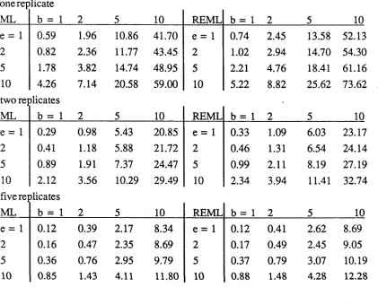
The variances o f e are equal under M L and REM L so only the values o f Var(b) are

given in Table 4.1.

Table 4.1 Var(b) for unbalanced experiments

one replicate

ML b = 1 2 5 10 REML b = 1 2 5 10

e = 1 0.59 1.96 10.86 41.70 e = 1 0.74 2.45 13.58 52.13

2 0.82 2.36 11.77 43.45 2 1.02 2.94 14.70 54.30

5 1.78 3.82 14.74 48.95 5 2.21 4.76 18.41 61.16

10 two ret

4.26 ilicates

7.14 20.58 59.00 10 5.22 8.82 25.62 73.62

ML b = 1 2 5 10 REML b = 1 2 5 10

e = 1 0.29 0.98 5.43 20.85 e = 1 0.33 1.09 6.03 23.17

2 0.41 1.18 5.88 21.72 2 0.46 1.31 6.54 24.14

5 0.89 1.91 7.37 24.47 5 0.99 2.11 8.19 27.19

10 five rej

2.12 ilicates

3.56 10.29 29.49 10 2.34 3.94 11.41 32.74

ML b = 1 2 5 10 REML b = 1 2 5 10

e = 1 0.12 0.39 2.17 8.34 e = 1 0.12 0.41 2.62 8.69

2 0.16 0.47 2.35 8.69 2 0.17 0.49 2.45 9.05

5 0.36 0.76 2.95 9.79 5 0.37 0.79 3.07 10.19

10 0.85 1.43 4.11 11.80 10 0.88 1.48 4.28 12.28

4.4 ILLUSTRATION WITH REAL DATA

Splus functions to calculate the variance of estimates of components of variance are at (A2.9) - (A2.10). They are written in terms of matrices rather than using, for example, (4.5), because they look more elegant and matrices are a more general way of expressing the calculations involved.

For the soybean data (see §2.1) F“1 _-0.93 4.65 —0.93 N _4.68

J

j

The next chapter completes the discussion of ML and REML estimation for normally- distributed data by examining distributions of estimates using a Monte Carlo experiment.

5. MONTE CARLO STUDY

For this Monte Carlo study, two variance component models were considered with

( I5

V

1 5 ;

(balanced) or Z fl5

V

15

J

(unbalanced). (5.1)

The variance components were chosen to be e = 4 and b = 16. By estimating e and b and examining the expected value, variance and number of iterations required to find the estimates, we can compare the performance of Anderson’s and Henderson’s algorithm. We can also examine the distributional properties of the estimates.

5.1 EXPECTED SUMMARY STATISTICS

Firstly, we use the fact that all MLEs (including REMLEs) 0 are asymptotically normally distributed with mean E(0) and variance [-E (32L/3030T)]_1 to produce a table of expected results (Table 5.1) to compare with the simulated results.

The variances of MLEs and REMLEs from both balanced and unbalanced experiments are calculated using Splus functions (A2.9) and (A2.10), which were introduced in Chapter 4.

To find the expected value of MLEs, start with (3.1) and take expected values. Thus E(0) = B '1 E(d)

/tr[V-2] tr[V GV ] \

^trtV 'G V "1] tr[V_1GV_1G]

-1 ftr[P]

tr[PG]

Expressions in e, m and b can be substituted for the traces so that for balanced data

f e2 - e 2 n - p m(n - p)

- e 2 I f e2 ^m (n - p) m i n - p

f n(e + ( m - l)b) - e e(e + mb)

(e + mb)2 P

J A

n - m e + mb

\

E(e) = n

(n - l)e + n(m - l)b

e(e + mb) m(n - p)(e + mb) e2(n - m)

_ me((n - l)e - e(p - 1) + n(m - l)b) m(n - p)(e + mb)

_ e((n - p)e + m(n - p)b) (n - p)(e + mb) = e (unbiased)

- _ -ne((n - l)e 4- n(m - l)b) (n - m)(ne2 + 2(n - p)meb + (n - p)m2b2) mn(n - p)(e + mb) m(e + mb)n(n - p)

_ (nb - mb - e)(n - p)(e + mb)

The expectations for unbalanced MLEs follow a similar pattern and are calculated using the Splus function (A 2 .ll). All REMLEs are unbiased, which can be derived from (3.2) and checked using (A2.12).

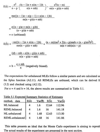
For e = 4 and b = 16, the above results are summarised in Table 5.1.

Table 5.1 Expected Summary Statistics of Estimates method, data E(e) Ward) E(b) Var(b) ML balanced 4 1.6 12.64 112.96 RE ML balanced 4 1.6 16 141.18 ML unbalanced 4 1.68 12.63 113.50 RE ML unbalanced 4 1.68 16 141.86

This table presents an ideal that the Monte Carlo experiment is aiming to reproduce. The actual results of the experiment are presented in the next section.

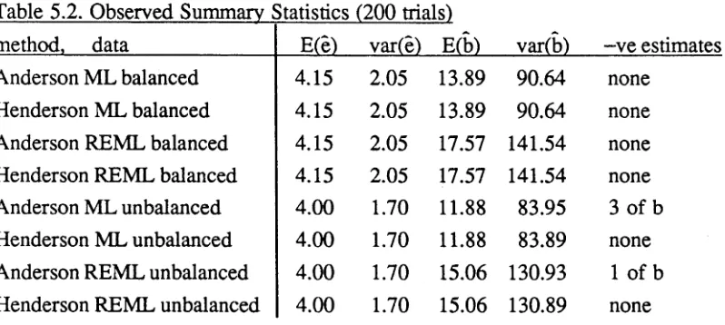
Table 5.2 lists the observed expected values and variances of 200 estimtes of e and b for the two experimental designs and two algorithms under consideration, obtained using the Splus functions (A2.13) - (A2.15). The distributions of the estimates are

n(n - p)(e + mb)

= b - e + mb (negatively biased). n

5.3 OBSERVED SUMMARY STATISTICS

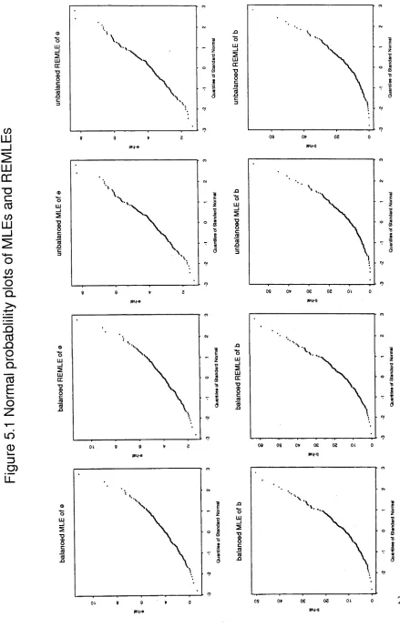
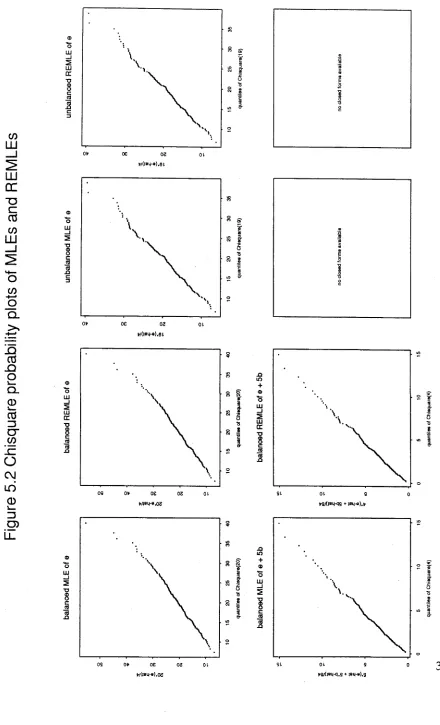
displayed in Figures 5.1 and 5.2. In Figure 5.1, the estimates are compared with the normal distribution; in Figure 5.2, linear combinations of the estimates are compared with

x

Table 5.2. Observed Summary Statistics (200 trials)

method, data E(e) var(e) E(b) var(b) -ve estimates

Anderson ML balanced 4.15 2.05 13.89 90.64 none

Henderson ML balanced 4.15 2.05 13.89 90.64 none

Anderson REML balanced 4.15 2.05 17.57 141.54 none

Henderson REML balanced 4.15 2.05 17.57 141.54 none

Anderson ML unbalanced 4.00 1.70 11.88 83.95 3 of b

Henderson ML unbalanced 4.00 1.70 11.88 83.89 none

Anderson REML unbalanced 4.00 1.70 15.06 130.93 1 of b

Henderson REML unbalanced 4.00 1.70 15.06 130.89 none

A smaller Monte Carlo study was also undertaken to determine the average number of iterations (to the nearest integer) required for convergence of the two algorithms in the four estimation situations (balanced or unbalanced data; ML or REML estimation). Table 5.3 lists the results.

Table 5.3. Average number of iterations required for convergence (5 trials)

data method # iterations data method # iterations

balanced Anderson ML 2 unbalanced Anderson ML 3

Henderson ML 8 Henderson ML 8

Anderson REML 2 Anderson REML 3

Henderson REML 7 Henderson REML 7

5.3 DISCUSSION

Figu

re

5.

1

N

o

rm

a

l

pr

o

ba

b

lil

it

y

p

lo

ts

o

f

M

L

E

s

a

n

d

RE

ML

Es

Figu

re

5

.2

C

h

is

qu

ar

e

p

ro

ba

b

ili

ty

p

lo

ts

o

f

M

L

E

s

a

n

d

R

E

M

L

E

s

WlBLI-o.03

i

■8

Table 5.3 shows that Anderson’s algorithm always converges more quickly, so that neither algorithm is clearly preferable over the other.

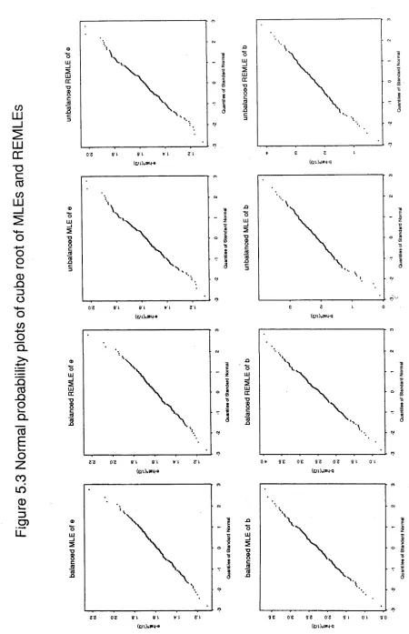
Comparing Table 5.1 with Table 5.2, we see that the observed summary statistics are within about 20% of their theoretical values, and some e.g. unbalanced E(e), are exact. However, the Normal probability plots (Figure 5.1) display distinct curvature, indicating non-normal distributions. The plots of sorted linear combinations of observed estimates against y} quantiles (Figure 5.2) are, in general, much straighter, indicating that the quantities plotted are distributed as y } variables. Furthermore, as shown in Figure 5.3, taking the cube root of the estimates induces near-normality in the distribution of the estimates. Thus it may be more appropriate for inferential purposes to work with the transformed estimates, rather than the raw ones.

The smallness of the experimental designs in (5.1) is probably the reason why the large-sample normal distributions do not seem to hold, but the small-sample y}

distributions do hold quite well. The effect of having such a small design is that e is being estimated with fewer than 30 degrees of freedom (observations) and b with, in effect, p - 1 = 4 degrees of freedom.

Thus this part of the thesis, dealing with estimation for normally distributed data, concludes with a lesson in experimental design. If components of variance are the parameters requiring estimation, it is advisable to have as many treatments as possible, even if this entails reducing the number of observations per treatment.

F

ig

u

re

5

.3

N

o

rm

al

p

ro

b

a

b

lilit

y

plo

ts

o

f

c

u

b

e

r

o

o

t

o

f

M

L

E

s

a

n

d

REMLE

s

cn

' I

6. NON-NORMALITY

2

So far we have always assumed that the random factors ß and e come from a N(0, o “)

distribution. This normality assumption allows the development of the variance matrices in Chapter 4, where it was found that for the one-way model, REML is asymptotically efficient for both balanced and unbalanced designs.

This chapter will address the questions: what happens to the size of the variances of the estimates when the data is non-normally distributed; does the MSE of the estimates behave in a similar way; and what is the asymptotic behaviour of the MSEs in the presence of non-normality?

6.1 VARIANCES FOR NON-NORMAL DISTRIBUTIONS: GENERAL CASE

The assumed distribution of the data is f(y, 0), but the actual distribution is g(y, 0). Then

E(0L/30) = E(3logf/50) = J(3f/30)/f(0) g dy and

E 0 2L/aeaeT) = J (-i/f)20f/ae)(3f/59)T + (i/f)(32f/aeaeT) g dy.

So var(9) = [E 0 2L/a939T)r'[E 0 L /a9 )0 L /a9 )T][E 0 2L/3939, ) r 1 (6.1) using the same Taylor series argument as §4.1. Calculation of the matrix (6.1) is the aim of the next section.

The particular non-normal distribution, g, considered in this thesis is the contaminated normal i.e. with probability 1 - So, £ ~ N(0, e) and with probability 5o, £ - N(0, koe), where ko > 1. Thus Var(e) = (1 - So + 5oko)e = e*.

Similarly Var(ß) = (1 - 8] + 5iki)b = b*. (6.2)

Clearly observations from this contaminated normal have variance E(y - Xa)(y - Xa)

/e* + b* b* 'N

— y * — _{So long as ß and £ are independent, V* will have the}

\ b * e* + b*

J

same structure as V whatever contaminated normal distribution is considered: simply denote the actual variances of £ and ß by e* and b*.

6.2 ONE-WAY UNBALANCED MODEL VARIANCE MATRIX 6.2.1 ML

The variance matrix as a whole is

^E(32L/3e2)

vE(32L/3e3b)

E(32L/3e3b) \ _ j

E(32L/3b2) j

/E(3L/3e)2

,E(3L/3e)(3L/3b) /E(32L/3e2)

JE(32L/3e3b)

E(3L/3e)(3L/3b) x

E(3L/3b)2 j

E(32L/3e3b) x _ t

E(32L/3b2) ,

(6.3)

The expectations that constitute (6.3) are

E(32L/3e2) = E [(-l/2)tr[V '(32V/3e2) - (V'‘(3V/3e))2]

+ (l/2)(y - X a)TV"'((32V/3e2) - 2(3V/3e)V'10V /3e))V 'I(y - Xa)]

= (l/2)tr[V"2] - tr [ V - 3V*] (6.4)

E(32L/3b3e) = E [(-l/2)tr[V '(32V/3b3e) - V '(3V /3b)V ‘(3V/3e)]

+ (l/2)(y - X a)TV '((32V/3b3e) - 2(3V/3b)V1(3V/3e))V,(y - Xa)]

= (l/2)tr[V ,G V 1] - tr[V"'GV_2V*] (6.5)

E(32L/3b2) = E[(-l/2)tr[V"(32V/3b2) - ( V ‘(3V/3b))2]

+ (l/2)(y - X a)TV"((32V/3b2) - 2(3V/3b)V'1(3V/3b))V'(y - Xa)] = (l/2)tr[V 'G V G ] - tr[V"'GV"'GV"'V*]. (6.6)

E(3L/3e)2 = E[(-l/2)tr[V"'(3V/3e)] + (l/2)(y - X a)TV'(3V /3e)V'(y - Xa)]2 = (l/4)(tr[V '])2 + (l/4)tr[V-2V*]tr[V-2V*] + (l/2)tr[V"2V*V-2V*]

- (1 /2)tr[V-']tr[V—2V*] (6.7)

E(3L/3e)(3L/3b) = E[(-l/2)tr[V'(3V/3e)] + (l/2)(y - X a)TV ‘(3V/3e)V‘(y - Xa)] [(-l/2 )tr[V ‘(3V/3b)] + (l/2)(y X a)TV '(3V /3b)V (y - Xa)] = (l/4 )tr[V ‘]tr[V''G] - (l/4)tr[V ‘]tr[V"GV‘V*]

- (l/4)tr[V"'G]tr[V~2V*]

+ (1 /4)tr[V_2V*] tr[ V~'G V ‘V*] + (l/2)tr[V-2V*V'GV'V*] (6.8)

It is no longer true that, for example, E(32L/3e2) = -E (3 L /3 e)2. However, it is true that letting V* = V in (6.4) - (6.9), the expected values equate to the expectations in the normally distributed case (§4.2.1).

6.2.2 RE ML

The calculations for REMLEs follow a similar pattern to those just given for MLEs. The variance matrix as a whole is:

/E(32L i/3 e 2)

vE(32Li/3e3b)

E(32Lj/3e3b) \ _-1 rE (3L]/3e)2 E(3Li/3e)(3Lj/3b) \

E(32Li/3b2) ^E(3Li/3e)(3Li/3b) E (3L i/3b)2 /E (32L i/3 e 2) E(32Li/3e3b) \ j

^E(32L]/3e3b) E(32Li/3b2)

and the elements of the matrices are:

E(32L ]/3 e 2) = E [(-l/2 )tr[P (3 2V /3e2) - (P 0 V /3 e))2]

+ (l/2 )(y - X6t)TV '((3 2V /3e2) - 2 0 V /3 e )P (3 V /3 e))V ‘(y - Xct)] = (l/2 )tr[P 2] - tr[V 'PV "(V * - X(XTV*‘'X )''X T)] (6.10)

E(32L i/3b3e) = E [ ( - 1 /2)tr[P(32V/3b3e) - P(3V/3b)P(3V/3e)l

+ (l/2 )(y - Xct)TV ( ( 3 2V/3b3e) - 2(3V/3b)P(3V/3e))V-'(y - Xöt)] = (l/2)tr[PG P] - tr[V"'GPV"‘(V* - X(X TV * ''X )'‘X T)] (6.11)

E(32L i/3 b 2) = E [(-l/2 )tr[P (3 2V/3b2) - (P(3V/3b))2]

+ (l/2 )(y - X6t)TV ',((32V /3b2) - 2(3V /3b)P(3V /3b))V ’(y - X6t)] = (l/2)tr[PG PG ] - tr[V 'G P G V '(V * - X (X TV *''X )_1X T)]. (6.12)

E (3L i/3e)2 = E [(-l/2)tr[P (3V /3e)] + (l/2 )(y - X ä )TV '(3 V /3 e ) V (y - X&)]2 = (l/4)(tr[P])2 - (l/2)tr[P ]tr[V -2(V* - X(XTV * ''X )''X T)]

+ (l/4 )(tr[V "2(V* - X(XTV * ''X )'‘X T)])2

+ (l/2 )tr[(V -2(V* - X(XTV*-‘X )'IX T))2] (6.13)

E (3L i/3e)(3L i/3b) = E [(-l/2)tr[P (3V /3e)] + (l/2 )(y - X6t)TV*‘(3V /3e)V '(y - X&)] [(-l/2)tr[P(3V /3b)] + (l/2 )(y X6t)TV*‘(3V/3b)V-’(y - Xöt)]

= (l/4)tr[P]tr[PG] - (l/4)tr[P]tr[V'GV"'(V* - X(XTV*'‘X)''XT)] - (l/4)tr[PG]tr[V_2(V* - X(XTV*''X)‘‘XT)]

+ (l/4)tr[V-2(V* - X(XIV*‘1X)"'XT)]tr[V~1GV'1(V* - X(XTV*"X)"XT)] + (l/2)tr[V-2(V* - X(XtV*''X)''Xt)V G V '(V * - X(XTV*"X)“XT)] (6.14)

E(3Li/3b)2 = E[(-l/2)tr[P(3V/3b)] + (l/2)(y Xct)TV ,(3V/3b)V'(y - Xöt)]2 = (l/4)(tr[PG])2 - (l/2)tr[PG]tr[V"GV‘(V* - X(X, V*',X)"'X1)]

+ (1 /4)(tr[V~'GV‘‘( V* - X(XTV*''X)'‘XT)])2

+ (l/2)tr[(V"1GV‘1(V* - X(XTV*'‘X)'lXT))2]. (6.15)

As before, letting V* = V in (6.10) - (6.15) reduces these equations to the equations for normally distributed data in §4.2.2.

6.3 NUMERICAL RESULTS

Consider the variance of e and b (estimates of e = b = 1) when the contaminated variances e* = (1 - 8o + ko5o) and b* = (1 - Si + kqSi) = 1, 1.5, 2, 3, using the experimental designs (5.1). Thus we are assuming that the data is normally distributed with e = b = 1, but in reality it follows a contaminated normal distribution with e* and b* taking the range of values given above.

It would be possible to write down the expected derivatives (6.4) - (6.15) in terms of ni, . . . , np, e, b, e* and b*; gather the expressions into matrices and multiply to get the variance matrices. But the derivatives take a complex form and are not very illuminating. The matrix equations are more elegant, and they can easily be converted into computer code (see (A2.16) - (A2.17)) so that the quantitative effects of non­ normality can now be studied. Output from these functions for the values of e* and b* described above is presented in Tables 6.1 and 6.2.

Table 6.1. Var(e) for the given non-normal distributions

Bal. b* = 1 1.5 2 3 Unbal. b* = 1 1.5 2 3

e* = 1 0.10 0.10 0.10 0.10 e* = 1 0.11 0.11 0.11 0.11

1.5 0.12 0.12 0.12 0.12 1.5 0.12 0.12 0.12 0.12

2 0.16 0.16 0.16 0.16 2 0.16 0.16 0.16 0.16

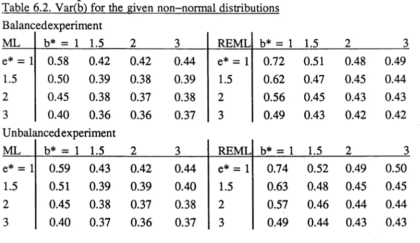
Table 6.2. Var(b) for the given non-normal distributions

Balancedexperiment

ML b* = 1 1.5 2 3 REML b* = 1 1.5 2 3

e* = 1 0.58 0.42 0.42 0.44 e* = 1 0.72 0.51 0.48 0.49

1.5 0.50 0.39 0.38 0.39 1.5 0.62 0.47 0.45 0.44

2 0.45 0.38 0.37 0.38 2 0.56 0.45 0.43 0.43

3 0.40 0.36 0.36 0.37 3 0.49 0.43 0.42 0.42

Unbakmeed experiment

ML b* = 1 1.5 2 3 REML b* = 1 1.5 2 3

e* = 1 0.59 0.43 0.42 0.44 e* = 1 0.74 0.52 0.49 0.50

1.5 0.51 0.39 0.39 0.40 1.5 0.63 0.48 0.45 0.45

2 0.45 0.38 0.37 0.38 2 0.57 0.46 0.44 0.44

3 0.40 0.37 0.36 0.37 3 0.49 0.44 0.43 0.43

For small experiments, we prefer MLEs on the basis of efficiency since for both balanced and unbalanced data, Var(MLE of b) < Var(REMLE of b).

It is interesting to note that the variances under non-normality are often smaller than under normality. This may be a result of the chosen values of e, b, e*, b* and the small size of the experiment, or it may be a manifestation of a global conservativeness of variance component estimates in the presence of non-normality.

Consider as an alternative to the variance, the MSE of the estimates. To do so, we require the bias of each estimate, which for e, is E(e) - 1 = e* — 1. For REMLEs of b, the bias = b* - 1. On the other hand, small-sample MLEs of b are further biased so that for the experimental designs (5.1) and the chosen values of e* and b*, the bias is

balanced___________________________________________ unbalanced

E(b) - 1 X> * II _{1.5 2 3 b* = 1 1.5 2 3}

e* = 1 -0.24 0.16 0.56 1.36 -0.2419 0.1581 0.5580 1.3580

1.5 -0.26 0.14 0.54 1.34 -0.2629 0.1371 0.5371 1.3371

2 —0.28 0.12 0.52 1.32 -0.2838 0.1162 0.5161 1.3161

3 -0.32 0.08 0.48 1.28 -0.3256 0.0743 0.4743 1.2742

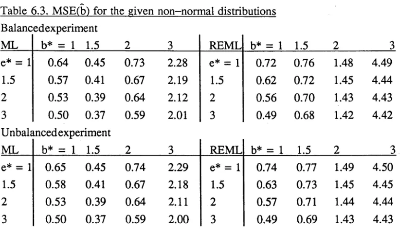
Adding the squared bias to the variances, the MSE is as shown in Table 6.3. MSE(e) need not be considered because MSE(MLE of e) = MSE(REMLE of e) in the presence of non-normality (cf. Table 6.1).

Table 6.3. MSE(b) for the given non-normal distributions Balancedexperiment

ML b* = 1 1.5 2 3 REML b* = 1 1.5 2 3

e* = 1 0.64 0.45 0.73 2.28 e* = 1 0.72 0.76 1.48 4.49

1.5 0.57 0.41 0.67 2.19 1.5 0.62 0.72 1.45 4.44

2 0.53 0.39 0.64 2.12 2 0.56 0.70 1.43 4.43

3 0.50 0.37 0.59 2.01 3 0.49 0.68 1.42 4.42

Unbalcmeed experiment

ML b* = 1 1.5 2 3 REML b* = 1 1.5 2 3

e* = 1 0.65 0.45 0.74 2.29 e* = 1 0.74 0.77 1.49 4.50

1.5 0.58 0.41 0.67 2.18 1.5 0.63 0.73 1.45 4.45

2 0.53 0.39 0.64 2.11 2 0.57 0.71 1.44 4.44

3 0.50 0.37 0.59 2.00 3 0.49 0.69 1.43 4.43

The overall pattern of Table 6.2 is retained: MSE decreases as e* increases for a given b*, while a generally increasing pattern is observed as b* increases for a given e*.

6.4 ASYMPTOTIC BEHAVIOUR

By replicating the experimental design as was done in §4.3.2, we may gain some insight into the asymptotic behaviour of MLEs and REMLEs of b and may see if the asymptotic efficiency of REMLEs carries over to the non-normal situation. Given the various biases involved, it is probably better to continue comparing MSEs.

Table 6.4 Asymptotic behaviour of MSE(b) two replicates of balanced design

ML b* = 1 1.5 2 3 REML b* = 1 1.5 2 3

e* = 1 0.30 0.36 0.89 3.15 e* = 1 0.32 0.52 1.29 4.33

1.5 0.27 0.33 0.84 3.07 1.5 0.28 0.49 1.26 4.29

2 0.25 0.32 0.82 3.03 2 0.25 0.48 1.25 4.28

3 0.24 0.30 0.79 2.95 3 0.23 0.49 1.25 4.27

five re]ilicates

ML b* = 1 1.5 2 3 REML b* = 1 1.5 2 3

e* = 1 0.12 0.33 1.02 3.75 e* = 1 0.13 0.40 1.20 4.26

1.5 0.10 0.31 0.99 3.71 1.5 0.11 0.38 1.17 4.22

two replicates of unbalanced design

ML b* = 1 1.5 2 3 REML b* = 1 1.5 2 3

e* = 1 0.31 0.36 0.89 3.15 e* = 1 0.32 0.52 1.30 4.34

1.5 0.27 0.33 0.84 3.07 1.5 0.28 0.50 1.26 4.30

2 0.25 0.32 0.82 3.02 2 0.26 0.49 1.26 4.28

3 0.24 0.30 0.78 2.94 3 0.23 0.49 1.25 4.28

five re]riicates

ML b* = 1 1.5 2 3 REML b* = 1 1.5 2 3

e* = 1 0.12 0.33 1.03 3.76 e* = 1 0.13 0.40 1.20 4.26

1.5 0.11 0.31 0.99 3.71 1.5 0.11 0.38 1.17 4.22

2 0.10 0.31 0.98 3.68 2 0.10 0.38 1.17 4.21

3 0.11 0.31 0.97 3.64 3 0.10 0.39 1.17 4.20

For a given value of b*, as e* increases MSE still decreases. No explanation for this phenomenon can be found, except that it corresponds to a situation where the random variation is swamping the systematic variation - not an ideal experimental situation in which to be. At least we can say that for small values of e* and b*, the MSE of REMLEs in the presence of non-normality approaches the MSE of MLEs in the presence of non-normality, for both balanced and unbalanced designs.

In order to allow for this effect of non-normality when interpreting the variance of estimates, we need ways to identify non—normality in data. The diagnostic tests discussed in Chapter 7 are some suitable solutions.

7. DIAGNOSTIC TESTS

Diagnostic tests cover a wide range of techniques, some graphical, some numerical. In all cases the aim is to detect outlying or influential observations in the data. To date, very few articles have appeared specifically devoted to diagnostic tests for the variance component model. Therefore this chapter contains a brief review of current diagnostic tests, and the extension of these tests to the variance components model. Splus functions (A2.18) - (A2.25) and the soybean data are used to illustrate each test.

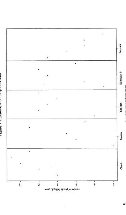
7.1 SCATTERPLOT OF OBSERVATIONS

The observations are plotted on the y-axis (Figure 7.1). The ordering along the x - axis is not important so long as points from the same treatment are grouped together. From this very simple plot we can try to see whether the spread is similar across the treatments i.e. whether the ßi are all from a N(0, b) distribution, and whether the within-treatments spread is larger than the between-treatments spread i.e. whether e > b. It does indeed seem to be the case here that e > b, but it is hard to tell if the spread is similar over all five treatments.

7.2 Q-Q PLOTS

For variance components models, where we assume ß ~ N(0, b), it will be of interest to compare each treatment’s observations with all the others. If all the treatment effects are from the same distribution, each Q-Q plot will lie close to a straight line. If none of the plots associated with the ith treatment follow this pattern, then the ith treatment effect may not come from the same distribution as the others.

This is not the standard format for Q-Q plots, where the order statistics of one sample of independent observations are plotted against the order statistics of a second independent sample. The observations for each treatment in a variance components model are not independent, but (in theory) they have the same dependence structure, thus the interpretation of the Q-Q plots remains as above.

F

ig

u

re

7

.1

S

c

a

tt

e

rp

lo

t

o

f

s

o

y

b

e

a

n

d

a

ta

£

<D

(/)

-Q

mojB 0} ßui|!B| sjuB|d jo jeqwnu

F ig u re 7 .2 Q -Q p lo t o f a ll p a ir s o f tr e at m en ts : so y b e a n d a ta § E? ® CO <D 6

uoßjeds jp UBsetues e}ewje-j

S

e

m

e

7.3 FITTED EFFECT PLOTS

Whereas Q-Q plots require only the raw data, fitted effect plots are drawn after e and b have been estimated. The p values of ß = DZTV_1(y - Xa) plotted against the quantiles of a N(0,1) distribution should lie in a straight line, as should the n values of £ = y — X a - Zß. The observed errors £ are in fact the residuals for the variance components model.

Figure 7.3 shows the Normal probability plots of the estimated effects for the soybean data. Plots for both ML and REML are given, but they are very similar. The residuals include a number of outliers in the lower tail, but otherwise follow a reasonably normal distribution. It is rather hard to comment on the Q-Q plots of just five treatment effects because the number of points is so small: nevertheless, these graphs seem to display curvature i.e. non-normality.

7.4 REGRESSION-TYPE DIAGNOSTICS

Regression diagnostics come in two varieties - ones that asses influence (often based on deleting one observation at a time) and ones that assess outlyingness (various sorts of residuals). For the ordinary regression model y = Xß + e, where y is an n x 1 vector of observations and ß is a p x 1 vector of parameters, some regression diagnostics are:

1)Hat matrix diagonals hi = [X(XTX)_1XT]ii.

The ith data value is influential if hi is close to one. “Large” hi are greater than 2p/n. 2) DFBETASjj = scaled change in jth parameter estimate on deleting ith observation

_ ßi - ßrn

ä(i)V[(XTX)_1]jj

As is usual with statistics scaled by their variance, if | DFBETASij| > 2 then the ith observation is influential. DFBETAS is similar to another well-known measure of influence, Cook’s Distance.

det[&(0 (xfijXci))-1]

3) COVRATIO = det[&2 (XTX)-']

= ratio of determinants of covariance matrices before and after deleting ith observation.

The ith observation is influential if its covratio lies outside the interval [1 - 3p/n, 1 + 3p/n].

Figure 7.3 Normal probability plots of observed effects

Q-Q plot of ML residuals i.e. epsilon-hat

Quantiles of Standard Normal

Q-Q plot of ML treatment effects i.e. beta-hat

o ---c\i ' •

in

o ° ■

&

c ■

0 o •

E

"5 o 2 o ■

o

■ •

-1.0 -0.5 0.0 0.5 1.0

Quantiles of Standard Normal

Q-Q plot of REML residuals Q-Q plot of REML treatment effects

7.4.1 REGRESSION-TYPE DIAGNOSTICS ADAPTED FOR THE VARIANCE COMPONENTS MODEL

1) Hat matrix diagonals need to be redefined for the variance components model, using the fact that y = Hy.

Since y = X a + Zß + e for the variance components model y = X a + Zß

= X(XTV’1X)"lXTV"1y + ZDZTV-1(y - Xa)

= X(XTV"1X)"1XTV“1y + ZDZtV_1(I - X(XTV’1X)'1XTV"1)y = (X(XTV 'IX)"1XTV l + ZDZTP)y

Thus the new hat matrix Hi = X(XTV"1X)'1XTV_1 + ZDZTP. Ideally Hi should have the properties of H, listed below.

a) is Hi symmetric? No, because X(XTV'1X)~IXTV'1 is not symmetric. b) is Hi idempotent? No, because

= [X(XTV ',X r'X TV" + ZDZ'P][X(XTV‘1X)'IXTV I +ZDZTP] * Hi.

c) [Hijii—> 1 =* ith observation is influential? This is still true because y = Hiy.

d) balanced data => [Hi]p all equal? This is still the case for the variance components model, and in fact for the one-way model the hat matrix diagonals are the same for any observations that come from groups with the same np

e) Var(y) = kHi? This is not the case, because Var(y) = Var(Xa + Zß) = Var(X(XTV"1X)“iXTV"ly + ZDZTPy)

= (X(XTV"1X)"1XTV“1 + ZDZtP)V(X(XtV_1X)"1XtV"1 + ZDZtP)t

= X(XTV"1X)"1XT 4- ZDZtPZDZt since PVP = P * kHi.

Note also that the variance matrix is symmetric by definition, but it is not idempotent. There is in fact no reason why we should expect to retain the “nice” properties of the hat matrix under OLS, but at least the important diagnostic properties still hold. For the soybean data, the hat matrix diagonals do not tell us anything of interest because the experiment is balanced, and [Hi]ü = 0.14 for all i. Observations with high leverage would have [Hi]ü > 2p/n = 12/25 = 0.48.

2) DFBETASjj = scaled change in jth parameter estimate on deleting ith observation. Now the parameters of interest are e and b, which have been referred to together as 0.

ThusDFTOETASie = | ^ , DFTHETAS* =

where the variances are based on the variance matrices of Chapter 4 e.g. for ML