The tag location problem

by

Michael D. Sumner, B.Sc., B.Ant.Stud. Hons (Tas)

Submitted in fulfilment of the requirements for the Degree of Doctor of Philosophy

Institute of Marine and Antarctic Studies University of Tasmania

no material previously published or written by another person, except where due acknowledgement is made in the text of the thesis.

Signed:

Michael D. Sumner

Signed:

Michael D. Sumner

Sumner, M. D., Wotherspoon, S. J., and Hindell, M. A. (2009). Bayesian estimation of animal movement from archival and satellite tags. PLoS ONE, 4(10):e7324.

The following people contributed to the publication of work undertaken as part of this thesis:

Michael Sumner (50%), Simon Wotherspoon (25%), Mark Hindell (25%).

Details of the Author’s roles:

Wotherspoon and Sumner outlined the original mathematical and soft-ware approach. Wotherspoon was responsible for most of the mathemat-ical content of the manuscript. Sumner completed the software, ran the models and wrote the manuscript. Hindell advised on the ecological goals and context and provided the data.

We the undersigned agree with the above stated “proportion of work undertaken” for the above published and peer-reviewed manuscript contributing to this thesis.

Signed:

Supervisor

Institute of Marine and Antarctic Studies University of Tasmania

Date:

Signed:

Institute of Marine and Antarctic Studies University of Tasmania

This thesis provides an integrated approach to common problems with loca-tion estimaloca-tion for animal tracking. Many existing techniques confound problems of location accuracy with simplistic track representations and under-utilization of available data.

Traditional techniques such as speed filtering and time spent maps are illus-trated with a software package developed by the author with examples of location estimates from southern elephant seals. This software enables the application and exploration of various techniques that have previously not been available in a single solution. These include filtering, temporal gridding, projection transformation and GIS integration.

A novel Bayesian approach is introduced for the more general problems faced by different tagging techniques. This approach integrates all sources of data in-cluding movement models, environmental data and prior knowledge. This general framework is illustrated by application to satellite tag data and light-measuring tag data. Examples are used to detail the use of movement models with a powerful track representation model, and the application of raw light data for location estimation. Previously under-utilized sources of data are used to inform location estimates.

A method for applying light level geo-location within the framework is presented. This approach provides a primary location estimate for each twilight and utilizes all of the available data from archival tags.

These model runs result in very large databases of samples from Markov Chain Monte Carlo (MCMC) simulations and techniques for summarizing these for the variety of analysis outputs are illustrated. This system solves issues of location uncertainty with a full path representation and provides spatial maps of residency for multiple animals.

The relation between archival tag data and ocean circulation is used to extend the application of archival tag data for location estimation for diving animals in a manner similar to commonly used SST methods. Diving profiles from elephants seals are compared with 4D oceanographic datasets. Older tags are limited by problems with measurement lags for temperature—this problem is addressed with a proxy model for temperature at depth to ocean height.

Primarily, thanks to Simon Wotherspoon and Mark Hindell for constant encour-agement, guidance and patience. Supervision is crucial to this process and Simon and Mark are a crucial component of this work.

Thanks to Kelvin Michael and Corey Bradshaw for early encouragement and help. (Kelvin also deserves special thanks for ongoing meta-supervision).

Maria Clipppingdale for helping start the whole thing in the first place. Greg Lee for lakeside conversations and for pushing me beyond my first programming language. Gareth James ensured that I left Sydney long enough to actually start this work. Toby Patterson for many conversations and emails, and specific guidance on early drafts and ideas. Aleks Terauds for lots of feedback and encouragement from the very beginning.

Jeremy Sumner and Sarah Cupit for constant support and encouragement, and helpful reviews on final drafts. David Pointing was a terrific office mate and remains a very good friend. Dave Procter and Edith O’Shea for being keen to hang out whenever we can.

John Corbett, Brett Muir, Sean Malloy, Steve Harwin and the Eonfusion team for a terrific work environment. Brett Muir provided an invaluable review at the last minute. The timeliness and attention to detail was incredibly helpful.

Mary-Anne Lea for so much enthusiasm and helpful feedback. Matt Dell for constant goodwill and for being a great mate. Michael O’Shea and Sean Malloy for helping build an awesome carpet burner. Students and colleagues at the Antarctic Wildlife Research Unit, WANKERS for life. Especially Judy Horsburgh, Michelle Thums, Virgina Andrews-Goff, Tim Reid, Iain Field, Caitlin Vertigan and Ben Arthur. Students and staff of IASOS, Maths and Physics and CMAR.

Dave Watts provided a whole swag of cool IDL code that helped me learn some of the mysteries of spatial and temporal data. John van den Hoff, Rachael Alderman, Jennifer Kingston Sinclair, Karen Evans, Chris Wilcox, Sophie Bestley, Kevin Redd, Kirk Buttermore, Klaus Engelberg, Roger Hill, Phil Ekstrom, John Gunn, Mark Bravington all provided specific wisdom and guidance.

There are a number of specific contributions of resources, code, data and knowl-edge that deserve special mention.

The following acknowledgements are specific to the published version of Chap-ter 3.

NCEP Reynolds Optimally Interpolated Sea Surface Temperature Data Sets were obtained from the NASA JPL Physical Oceanography Distributed Active Archive Center, http://podaac.jpl.nasa.gov. The 2-Minute Gridded Global Relief Data (ETOPO2) were obtained from the National Geophysical Data Center, Na-tional Oceanic and Atmospheric Administration, U.S. Department of Commerce, http://www.ngdc.noaa.gov. Solar position algorithms of Meeus (1991) were adapted from the Solar Position Calculator made available by the NOAA Surface Radiation Research Branch, http://www.srrb.noaa.gov/highlights/sunrise/azel.htm. Greg Lee and Toby Patterson provided helpful suggestions on an earlier draft. Helpful feed-back from two anonymous reviewers has been incorporated.

The R community is a force of nature and I owe a great debt to the creators and core developers of R, and to the very many package contributors. I greatly appreciate the efforts of colleagues and friends who have enthusiastically embraced this tool and helped me on the way. In particular I owe a debt of thanks Edzer Pebesma and Roger Bivand.

Manifold GIS and its awesome users for a lively and exciting community. Tim Callaghan provided the LaTeX template and styles for the entire structure of the document. This thesis was written mostly in Emacs with Sweave and R, using Subversion, BibTeX and JabRef. To build the document figures and displayed code I have used R 2.12.0 with the following packages: MASS, mgcv, deldir, spatstat, lattice, sp, rgdal, maptools, geosphere, zoo, maps, mapdata, RODBC and ff.

Any errors are of course mine and cannot be attributed to my very generous helpers. When something takes as long as this did there are lot of people to ac-knowledge. I have surely failed to mention everyone or to fairly pay my thanks so if this applies to you please accept my apologies and gratitude. It was appreciated. Norm, my best friend. Life is horrendously unfair and you improved mine im-mensely. I wish desperately that you could share the rest.

My mother and father for love and support, and providing me with everything I’ve ever needed.

Ross Ihaka and Robert Gentleman, 1996

In light of this, I’ve come to the conclusion that rather than “fixing” R, it would be much more productive to simply start over and build something better.

TABLE OF CONTENTS i

LIST OF TABLES iv

LIST OF FIGURES v

1 INTRODUCTION 1

1.1 The thesis . . . 2

1.2 Chapter outlines . . . 2

2 THE TAG LOCATION PROBLEM 4 2.1 Rand thetrip package . . . 5

2.2 Problems with location estimation . . . 5

2.2.1 What is a trip? . . . 7

2.2.2 Practical data issues . . . 8

2.2.3 Joining the dots . . . 10

2.2.4 Summary of problems . . . 12

2.3 Summarizing animal behaviour from point-based track data . . . 13

2.3.1 Filtering . . . 13

2.3.2 Non-destructive filtering . . . 18

2.3.3 Spatial smoothing—surfaces from track data . . . 18

2.3.4 Partitioning tracks and grids into time periods . . . 26

2.3.5 Map projections . . . 26

2.3.6 Tools for traditional methods . . . 29

2.4 The trip package for animal track data . . . 29

2.4.1 Generating trip objects . . . 30

2.4.2 Filtering for unlikely movement . . . 35

2.4.3 Creating maps of time spent . . . 40

2.5 The need for a more general framework . . . 43

2.5.1 Location estimation from raw archival data . . . 46

2.5.2 Filtering locations . . . 47

2.5.3 Intermediate locations . . . 48

2.6 Conclusion . . . 49

3 BAYESIAN ESTIMATION OF ANIMAL MOVEMENT FROM ARCHIVAL AND SATELLITE TAGS 50 3.1 Introduction . . . 51

3.2 Materials and Methods . . . 53

3.2.1 Ethics Statement . . . 53

3.2.2 Assumptions . . . 53

3.2.3 Satellite tags . . . 55

3.2.4 Archival tags . . . 55

3.2.5 Posterior estimation . . . 56

3.2.6 Examples . . . 57

3.3 Results . . . 59

3.3.1 Argos tag data set . . . 61

3.3.2 Archival tag data set . . . 64

3.4 Discussion . . . 67

3.4.1 Path . . . 67

3.4.2 Precision . . . 67

3.4.3 Latent estimates . . . 67

3.4.4 Combinations . . . 69

3.4.5 Updating the models . . . 69

4 LIGHT LEVEL GEO-LOCATION FROM ARCHIVAL TAGS 72 4.1 Light-based derivation techniques . . . 73

4.1.1 Fixed point methods . . . 73

4.1.2 Curve methods . . . 74

4.1.3 Aims of this study . . . 74

4.2 Methods . . . 76

4.2.2 Movement model . . . 80

4.2.3 Estimation . . . 80

4.3 Examples . . . 81

4.3.1 Discussion . . . 81

4.4 Conclusion . . . 88

5 REPRESENTATION OF TRIP ESTIMATES 89 5.1 Representation of location estimates . . . 90

5.2 Primary locations and intermediate locations . . . 91

5.3 Features of the representation scheme . . . 96

5.4 Examples . . . 96

5.5 Conclusion . . . 101

6 AUXILIARY DATA FOR LOCATION ESTIMATION 102 6.1 A problem of scale . . . 103

6.2 Data availability . . . 103

6.3 Slabs versus points . . . 105

6.4 Temperature applications . . . 105

6.4.1 Temperature profiles . . . 106

6.4.2 Ocean height proxy . . . 107

6.4.3 Masks . . . 109

6.5 Large data set example . . . 110

6.6 Conclusion . . . 111

7 CONCLUSION 112 A MARKOV CHAIN MONTE CARLO 114 A.1 Metropolis Hastings . . . 114

A.2 Example . . . 115

B ARGOS DATA ESTIMATION EXAMPLE 119 B.1 Argos data example . . . 119

3.1 Estimate precision for Argos data set Summary of precision calculated from the posterior for x by original Argos class (km). Each row presents a quantile summary for the CI ranges (95 %) from each Argos class for longitude and latitude. The seven classes are an attribute provided with the original Argos locations (Service Argos, 2004). . 64 3.2 Estimate precision for archival data set. Summary of precision

cal-culated from the posterior for x from the archival tag. A quantile summary for the CI ranges for longitude and latitude. . . 67

A.1 Comparison of exact and MCMC approximations for N = 500 sam-ples and N = 5000 samples for the Binomial example with n = 20 andy= 12. . . 118

2.1 Raw Argos estimates for a Macquarie Island elephant seal. The line connecting the points is coloured from blue through purple to yellow in order relative to the time of each position. (Macquarie Island can just be seen in black beneath the third dark blue line segment). The outward and inward journeys are much faster than the journey throughout the Ross Sea, as shown by the colour scale change. A graticule is shown for scale, 10 degrees on the main plot, and 20 degrees on the inset. . . 6 2.2 Land filter and Argos quality class filter. In the first panel any point

occuring on land has been removed, and in the second any point with an Argos class of quality <“B” has been removed. In each panel the state of the track prior to filtering is shown as a dotted line. The coloured filtered line uses the same time-based colouring as in Figure 2.1. . . 15 2.3 Recursive speed filter applied using the McConnell method to the

track data shown in Figure 2.1. The small panels show the RMS speed calculated for each point for two of the ten iterations of the filter. At each iteration any point with an RMS speed above the required maximum threshold speed (the horizontal line) is flagged (shown as ”x”) and removed. The RMS speed axis is logarithmic. The resulting filtered track is shown in the larger panel on the right with the same temporal colour scale as used in Figure 2.1. . . 17 2.4 Argos track filtered by penalizing by sum of squares speed. The

filtered track is shown with the same time-based colour scale as in Figure 2.1, and the unfiltered track is shown as a dashed line. The original data was used without resampling. . . 19 2.5 Argos filtered longitude and latitude from Figure 2.4 by penalized

sum of squares speed. The coloured lines use the same time-based colour scale as in Figure 2.1. The unfiltered longitude and latitude are shown as a grey line. . . 20 2.6 Track lines binned into a coarse grid, using a line segment value to

sum into each cell. Cells are coloured from light to dark blue for increasing values. The sum of values resulting from each smaller line segment is shown for each cell. . . 23

2.7 Track lines binned into a fine grid. The track and grid origin is the same as in Figure 2.6. The coarser grid outline is shown for occupied cells as thick black lines. . . 24 2.8 Side by side plots of line gridding and KDE gridding to a coarse grid.

The input line is shown at an arbitrary height above the cells. . . . 25 2.9 Side by side plots of line gridding and KDE gridding to a fine grid.

The input line is shown at an arbitrary height above the cells. . . . 26 2.10 Raw Argos estimates and penalized smoothed track plotted in raw

longitude and latitude. Great circles are drawn as curves, from Mac-quarie Island through the most distant raw Argos position (solid) and the most distant smooth position (dashed). . . 27 2.11 Raw Argos estimates and penalized smoothed track plotted in an

equal-area projection. Great circles (as-the-crow-flies) are shown as lines. These pass through the Macquarie Island site to the most dis-tant raw Argos position (solid) and the most disdis-tant smooth position (dashed). . . 28 2.12 Plot of Argos track data from a trip as points, with lines showing

the speed filtered tracks, coloured for each separate trip. . . 37 2.13 Originalsdafilter(red) and customtripspeed distance angle filter

(thick grey line). The original raw track is shown as a thin grey line. 41 2.14 Simple image of a time spent grid for the trip object. . . 42 2.15 Four variations on a tripGrid. grid.filteredandgrid.c026use the

simple line-in-cell method for all four seals and for seal c026 alone. kde3.filtered and kde1.filtered use the kernel density method for line segments with a sigma of 0.3 and 0.1 respectively. Each grid has dimensions 100x100 and time spent is presented in hours. . . 44 2.16 A relatively coarse version of fourgrids with a specific

kilometre-based cell size (80x60km), specified within an equal area map projection. 45 2.17 Light level geo-locations for black marlin in the Coral Sea. This image

is taken from Figure 3a in Gunn et al. (2003) and is reproduced with the permission of the authors. . . 48

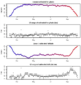
3.2 Estimates and time spent for archival data setPanel A: Poste-rior means forxfrom the archival data set plotted spatially, with time scale from red to blue. The sequence provides a realistic trajectory for an elephant seal. The dashed grey line shows the (approximate) position of the Southern Boundary of the Antarctic Circumpolar Cur-rent. Panel B: Map of time spent from full path estimates from the archival data set. Bin size is 5.5 km by 9.3 km at 54 S and 3 km by 9.3 km at 72 S. . . 61 3.3 Individual longitude, latitude estimates for Argos Posterior

means forx from the Argos data set for longitude and latitude, with time scale from red to blue as in Figure 3.1. The grey line shows the implied sequence of the original Argos estimates. Also shown is the range of the 95 % CI of each estimate (km), determined with the mean by directly summarizing the posterior. . . 63 3.4 Intermediate estimates for Argos Posterior means forx of longitude

and latitude for a short period (23-26 Feb 2006) with CI ranges shown. The CI range for intermediate estimates (full path) is shown as a continuous band. . . 65 3.5 Posterior means for archival data setPosterior means forxfrom

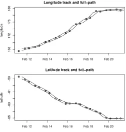
the archival data set for longitude and latitude, with time scale from red to blue as in Figure 3.2a. Also shown is the range of the 95 % CI of each estimate (km), determined with the mean by directly summarizing the posterior. . . 66 3.6 Intermediate estimates for archival data set Individual mean

estimates of longitude and latitude for a 10 day period in February with CI ranges shown, as well as the CI range for intermediate esti-mates (full path) shown as a continuous band. . . 68

4.1 Locations around Macquarie Island (158o 57’E, 54o 30’ S). Square icons indicate locations along the current twilight line, triangles in-dicate the corresponding “evening” locations. Macquarie Island is at the intersection of the two curves. . . 78 4.2 Morning twilight solar elevations for locations around Macquarie

Is-land from Figure 4.1 (squares). The time at which the elevation is 0 (sunrise) is indicated with a vertical line, and the horizontal lines show solar elevations -5 and 3. . . 79 4.3 Morning twilight solar elevations for location around Macquarie

Is-land from Figure 4.1 (triangles). The time at which the sun is at elevation is 0 (sunrise) is indicated with a vertical line, and the hori-zontal lines show solar elevations -5 and 3 . . . 79 4.4 Mean longitude and latitude values from the posterior, plotted with

surrounding 95% confidence intervals for elephant seal example. . . 82 4.5 Mean longitude and latitude values from the posterior, plotted with

4.6 Mean longitude and latitude values from the posterior, plotted with the 95% confidence intervals (closed circles) and the full binned esti-mate boundary (open circles) for the fur seal example. . . 84 4.7 Mean longitude and latitude values from the posterior, plotted with

the 95% confidence intervals (closed circles) and the full binned esti-mate boundary (open circles) for the elephant seal example. . . 85 4.8 Time spent estimate for entire trip derived from all posterior samples

for Macquarie Island elephant seal. . . 86 4.9 Time spent estimate for entire trip derived from all posterior samples

for Amsterdam Island fur seal. The zonally (east/west) oriented lines in the inset are mean locations of Southern Ocean fronts (Orsi et al., 1995). Only the Subantarctic front is seen in the main figure region. 87

5.1 (A) Simple track of three locations in a traditional representation, moving from left to right. The grey region is included to represent a boundary to the animal’s movement, such as a coastline. (B) The points represent unknown locations with some uncertainty. (C) A representation of these location estimates which are disconnected in time. (D) Connecting the measured locations are regions that are again unknowns with some uncertainty. . . 92 5.2 (A) Between the first two measured locations is a region of unknown

migration connecting the two end points, which can be rather wide. (B) The second connected region, more constrained relative to the first in terms of possible lateral movements. (C) Notation of xi for

primary estimates. (D) Notation ofzi for intermediate estimates. . . 93

5.3 Illustration of the grid index scheme. Two child grids are shown within the parent, with indicated index values. . . 94 5.4 Example showing a real child grid within a parent grid. The inset

window shows the detail of the grid. . . 95 5.5 A short region of an Argos track of a ringed seal in Newfoundland.

The primary estimates shown as contours are compared to the original Argos estimates. All but three Argos estimates have class “B” and are marked with “+”, the others are labelled with their classes “2” and “A”. The confidence in the “2” location is reflected by the proximity of the estimate to it and that it is relatively localized. None of the estimates fall on land like some of the Argos locations, and some are tightly bound by the land—but not clipped arbitrarily to it. . . 97 5.6 Original Argos track with sequence of modal locations from the

5.7 Individual intermediate estimates shown as contours with modal lo-cations from the primary estimates shown as dark “X” symbols (as in Figure 5.6). The intermediate estimates overlap the primary esti-mates in space as well as connecting them in time. . . 99 5.8 Time spent estimate from combination of the nine intermediate

esti-mates. This single surface is constructed by combining the separate intermediate estimates for the time duration, each weighted by their corresponding time interval. . . 100

6.1 Temperature and salinity profiles from two regions for an elephant seal track. Seal dive profile values are shown as a red line. The points are all data values from the profiles taken from the GEM model for the corresponding seal depths at the grid of locations shown. The first is near Macquarie Island, the second near Ad´elie Land. . . 108 6.2 Series of location likelihood maps based on SSH proxy from

temper-ature at-depth. . . 109

INTRODUCTION

Modern animal tracking analysis consists of a diverse set of techniques used by a wide range of researchers in many disparate fields of science. There are established tra-ditional techniques that range from very simplistic spatial representations of tracks (Samuel et al., 1985; Bradshaw et al., 2002; Croxall et al., 2004), to powerful sta-tistical models that rely on modern computing hardware for their solution (Jonsen et al., 2005; Patterson et al., 2008; Breed, 2008). There are significant divides be-tween fields in terms of the importance of certain techniques and in the access to existing tools. Some of these differences are due to the species being studied or the priorities of the research, and some are due simply to the established habits of a community or their access to the necessary tools.

In terms of the available software tools, there is a divide betwen the tool users and tool makers in that many of the problems involved with analysis do not come to light until algorithm development is attempted (Calenge et al., 2009). The major problems with estimates of tag location accuracy and reliability are well-understood, but the related issues of data consistency and management are rarely seen except by those who develop the software tools (Coyne and Godley, 2005; Halpin et al., 2006). Somewhat paradoxically, with widespread access of modern computing hardware and software, more researchers are exposed to the implementation details applied to raw data and track analyses and are required to act as practioners managing and analysing data (Block et al., 2003a; Hartog et al., 2009).

The availability of computing and visualization tools has provided the ability to scrutinize analyses against existing knowledge or intuition. Mapping tools en-able realistic representation of animal tracking analyses and can present insights or problems that were not initially apparent. There is great promise for accessible software to enable greater realism, or at least provide the representation of very complex models involving time-developing 3D with multiple variables of interest (Andres et al., 2009).

Animal tracking is a modern field that has seen great advances made with re-searchers working closely with tag manufacturers to ensure that tag development closely matches the priorities and requirements for data collection (Wilson et al., 2002; Afanasyev, 2004). This same improvement has been occurring with software tools as researchers “get their hands dirty” working with raw track data. The de-velopment of techniques like MCMC for the solution of Bayesian models provides

the ability to model very complex problems with spatial and temporal structure, involving large and disparate data sets (Dennis, 1996; Dixon and Ellison, 1996).

1.1

The thesis

By the application of Bayesian methods we can utilize all information sources to help with the variety of problems of location estimation for animal tracking. An investigation of traditional track methods shows that the point and line model is too simplistic and reveals a number of inherent problems. From this perspective we see that no matter the method, approaches that deal with tracks as a time series of points or lines are inherently limited, and that these limitations apply to data collected by a variety of tag types. Some process that generates a time series of locations has a deeper rawer source of data behind it and it is this that fits best in an integrated Bayesian approach.

This thesis considers problems with animal tracking data, focussing on the es-timation of location. There is some consideration of data handling, mostly from an estimation and quality control perspective. One of the main goals is to take advantage of the large collection of existing data sets, rather than attempt to design best methods for obtaining data. Traditional techniques are presented to illustrate the main problems involved with tag location analysis and provide a toolkit for executing these traditional techniques. Many researchers are aware of cutting-edge analytical techniques that are improving the outputs from tracking data, but access to these is often difficult and there is a lack of understanding of their limitations.

1.2

Chapter outlines

Chapter 2 provides an overview of general problems with the analysis of tracking data, assuming that we have location estimates to begin with. We look at the common features of tracking data and some of the common problems faced when using these data. The chapter provides a toolkit for dealing with tracking and associated data, pointing out some of the limitations when applying simple models to quality assurance. The chapter concludes with the need for integration of track analysis with the derivation of location from raw data, such as from archival tags.

Chapter 3 provides a general Bayesian framework for estimating location by app-plying any available data, prior knowledge and movement models. The theoretical approach is provided with examples of using the framework for two different data sets.

Chapter 4 presents the application of the Bayesian framework to an archival tag data set in full detail. A curve method for light level geo-location is introduced that provides the practitioner with open access to every component of the model in freely available tools.

THE TAG LOCATION PROBLEM

This chapter discusses problems faced with tracking data that concern the estimation of location and provides a flexible software environment for exploring data and applying solutions. Examples are used to illustrate the variety of problems and some of the limitations of the traditional techniques by which tracking data are analysed. The trip package is a dedicated suite of tools developed by the author in the software language R. This package integrates data handling and analytical techniques for track data with broader GIS and spatial data tools. This makes track data handling tools easily available, even for those without strong programming skills. The chapter concludes by extending the concerns regarding the limitations of traditional techniques to methods for deriving locations from raw data.

This chapter is not intended to be a critique of modern methods of dealing with tracking data, but introduces the variety of issues encountered and tools for applying them. Simple-to-use tools for handling spatial and temporal data are still rare and some of the problems encountered cause difficulties for researchers before they have an opportunity to explore sophisticated methods. The aim here is to illustrate some classical techniques within a software toolkit that provides better control over the details of analysis tools for those without advanced programming skills. Later chapters present solutions for the remaining problems. Work by Patterson et al. (2008) and Breed (2008) provide a more critical review of recent methods.

Aims of this chapter:

1. To introduce existing problems in tracking analyses presented with examples of classical techniques.

2. To illustrate the complexity of problems and areas that require more sophis-ticated solutions than traditional techniques. The problems presented here illustrate the need for solutions that come later in the thesis.

3. To present a flexible and readily customized software package as a framework for classical analyses and starting point for more sophisticated analyses.

4. To explain the compromises that are often made with regard to data rep-resentation and storage, as dictated by traditional systems, rather than an expressive model of the problem represented by the spatial and temporal data.

5. To encourage the use of techniques for automatic data validation, spatial and temporal data storage and integration with database and GIS technologies.

2.1

R

and the

trip

package

The software packagetripdeveloped with this chapter provides an integrated system for data validation and a development framework for track analyses. This can be used as a launching point for further analysis such as validating input to Bayesian methods, or filtering for state-space models (Patterson et al., 2010). As an extension of the Renvironment, trip also provides integration with tools for data access and output, integration with GIS and other data systems, and metadata for projections and coordinate systems. The trippackage ties together numerous tracking analysis techniques, which previously were only available though a wide variety of disparate tools, each having various requirements and limitations.

Thetrippackage was developed within the freely available software platformR, a statistical programming environment consisting of a vast community of contributing developers and users (R Development Core Team, 2010). Ris organized into modules known as packages which provide the functionality of the language, and also the mechanism by which it is extended1. New packages are created using the same tools by which R itself is built and can be contributed to a public repository such as the Comprehensive R Archive Network (CRAN2). The repository system for contributed packages is one of the great strengths of R and is part of the reason for its ease of use and subsequent popularity. The spatial and temporal capabilities of R are advanced, including strong integration with other technologies such as databases, GIS software and the wide variety of spatial and other complex data formats.

The tools provided in R for coercion between complex data types are very pow-erful, allowing rather different packages to share data with tight integration Bivand et al. (2008); Chambers (2008). There are some fundamental data representations required for spatial analysis and careful organization is needed to provide coercions between different types to get all the tools to work together. The underlying spatial tools used to create the trip package are described in Section 2.4 with examples of using the software.

2.2

Problems with location estimation

This section presents actual tag location estimates to illustrate common problems associated with track data. The location data were provided by System Argos, which is a worldwide satellite service that provides location estimates from small mobile transmitters.

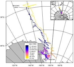
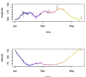
The first example is a sequence of Argos position estimates for a single elephant seal in Figure 2.1. All raw estimates provided are shown, with the longitude and latitude values transformed to an equal-area projection and drawn connected as a

1_{Seehttp://en.wikipedia.org/wiki/Package_Development_Process.}

2

date (1999) 01 January 28 January 23 February 21 March 16 April 13 May 08 June 04 July Macquarie

Island

65°S 55°S

120°W 140°W 160°W 180°W 160°E Ross Sea

Figure 2.1: Raw Argos estimates for a Macquarie Island elephant seal. The line connecting the points is coloured from blue through purple to yellow in order relative to the time of each position. (Macquarie Island can just be seen in black beneath the third dark blue line segment). The outward and inward journeys are much faster than the journey throughout the Ross Sea, as shown by the colour scale change. A graticule is shown for scale, 10 degrees on the main plot, and 20 degrees on the inset.

line. While there is obvious noise in the track, the general sequence of events is clear: the seal leaves Macquarie Island, swimming predominantly south-east to the Ross Sea where it spends several weeks, and then returns via a similar path in reverse.

There are a number of problems with the location estimates, some that are very obvious, but others that are more subtle. First, some of the dog-legs in the path seem very unlikely. On the outward journey the blue path shows some lateral movement to the west and east, and just before the return to Macquarie Island there is a similar movement to the west, then east. These are obvious problems seen as noise in the track, with positions that cannot be believed that do not otherwise obscure the general pattern of movement. Other dog-legs in the path are less extreme, so are more plausible.

difficult to evaluate. A location on land may be plausible if it is near enough to the coast, though this can interact with further issues requiring interpretation. These include that the start and end location are not exactly at the known “release” and “re-capture” sight, which was the isthmus at Macquarie Island. This isthmus is quite narrow and is readily crossed by elephant seals, though regions of the island to either side of the isthmus can only be traversed by sea. Another section of the track at the beginning has the path of the animal crossing Macquarie Island itself. At the scale of this image this inaccuracy seems unimportant since the island is such a small area within the study region. However, if the region of land concerned was a much larger peninsula then the problem of choosing which region was actually visited remains.

A scheme that proposes to remove or correct extreme positions faces the problem of defining appropriate thresholds. “Extreme” dog-legs cannot simply be discarded as the question of what is “too-extreme” does not have a simple answer. A simple rule to discard any location on land will not work since these animals do actually visit coastal regions. The distance that a seal might travel inland is not very far but depending on the species studied and the environment the situation may not be so clear-cut.

There are other issues of plausibility. For example, the coastline in the figure is quite coarse and while it may be sufficient for the scale of the image it does not represent the actual coastal boundary available to the seal. The real coastline is far more tortuous, detailed and dynamic—and may be significantly different from a particular data set due to the current fast- or sea-ice cover. This is a general issue with any data set available for informing models of animal location—the assumptions and limitations must be understood and used appropriately.

In terms of the incorrect first and last positions in Figure 2.1, these could be updated to be the actual release and recapture sites, but it might be more correct to actually add those locations and times to the start and end of the sequence of records. This is a data consistency issue that leads to the next family of problems in track data.

2.2.1 What is a trip?

There are a number of practical issues associated with the organization of track data that can present more prosaic problems. This section discusses some terminology and suggests the use of a “trip” as the unit of interest and that can be defined with database-like validation restrictions. The idealization of an animal’s trip is a continuous line in four dimensional space-time that is perfectly accurate as a representation of the seal’s position. For practical reasons, this ideal case can only be represented as a series of point samples of uncertain accuracy, in two or three spatial dimensions parameterized by time.

and terrestrial species are provided by Cooke et al. (2004), Wilson et al. (2002) and Kenward (1987).

Archival tags record and store data that is later retreived from the tag, while remotely sensed tags emit an electromagnetic or acoustic signal that is detected by an installed system of sensors, such as a satellite or acoustic array. (This categorization is not always maintained in practice, as archival tags may be satellite-linked in order to upload data in near real-time, but for the purpose of location estimation the distinction holds for the types of available data).

A loose set of definitions then is:

tag the device put on the animal.

track data any temporally referenced location data resulting from a device at-tached to an animal.

trip a specific tracking “interval” where a tag was attached, the animal is released for a time, and the tag (or just its data) is eventually retrieved. A trip may be represented in some way with track data that has some quality control or modelling applied.

Data resulting from the tagging process are identified by the device ID, as well as by the identity of the individual animal the tag is attached to. The same tag might be put on different animals, or the same animal might have been tracked on two or more separate occasions. For central-place foragers, a single tagging event may involve the same animal leaving the tagging site and returning multiple times. Once the interval of interest is defined it can be regarded as a trip. A single leave / return or a tag deployment / retrieval may be referred to as a trip. Whether multiple leave / return events are considered within a single trip depends on the research question—migratory animals usually won’t have such clear trip boundaries as central-place foragers, for example. The difference is important as the behaviour of interest for central-place foragers is primarily between leave / return events, and the return event is usually the only opportunity to retrieve a tag. Finally, there may not be data for the entirety of the trip of interest due to tag loss or memory restrictions, and so require the inclusion of trip sections where location is uncertain or completely unknown.

For the current discussion, define a trip to coincide with the interval of interest for which there is useable data from the tagging process. “Tracks” or “track data” then are just a set of location and other data, with no particular organization or quality control.

2.2.2 Practical data issues

subsequent records are acceptable. Duplicates in time do not make sense since either they are redundant copies of a previous record, or there is an implied infinite speed. These are common from the Argos Service, an example is found in the seal data example given by Freitas (2010) which is used in Section 2.4.2.3 Analytical meth-ods sometimes apply a non-zero time difference arbitrarily to avoid divide-by-zero errors. Less serious is the issue of successive duplicate locations, but care must be taken when calculating metrics such as speed based on inter-point distances. Each of these cases should be investigated carefully in case they hide errors from other causes such as mistaken data handling.

Missing values must also be handled carefully. Location and time coordinates cannot be used if they are missing or non-finite, even if their record appears in the correct order. Missing values can arise in a number of ways—infinities or undefined numeric values from numeric errors, or out of bounds coordinates, transformation errors, data missing from a regular sequence—and the exact reasons need to be carefully understood.4 This is a different approach taken to that of Calenge et al. (2009) who explicitly allow missing coordinates as part of “trajectories”. This is most pertinent in the context of tracks of regular time intervals where a missing point can be significant in terms of interpretation. The definitions here are not intended to determine which approach is more appropriate and there is no reason the two rationales cannot co-exist, but the current implementation in the trippackage disallows missing coordinates.

From a programming perspective, the use of rigid classes (definitions) with valid-ity checking can significantly reduce the time wasted solving these problems (Cham-bers, 1998). Based on the above, the minimal data-consistency preparation required can be achieved in the following way. Read all records, sort by trip ID then date-time, remove duplicated records or records with missing or non-numeric spatial or temporal coordinates. (The definition of “invalid” for a coordinate may involve out of bounds values such as those for longitude and latitude, but this step only refers to the data values, not their interpretation). Remove or adjust any records with duplicate date-times within a single trip ID. Up to this point no interpretation has been applied to the data—this will provide a useable set of records that can pass minimal validation but each step should be carefully investigated to ensure that automated decisions are not introducing new errors.

One way to adjust duplicate times is to simply modify the values forward or back by a small amount, but this can be problematic depending on the time differences involved. The reason for duplicated times is more likely to be a problem with the data itself and should be investigated.

Other problems in this regard deal with the sensibility of movements in a par-ticular coordinate system. The most commonly used coordinate system for tracking data is longitude and latitude on the WGS84 datum. For animals that traverse

3

Another recent example of duplicated times in a GPS data set is discussed here: http://lists. faunalia.it/pipermail/animov/2010-August/000635.html

4

hemispheres and cross critical meridians such as the Pacific Ocean dateline (longi-tude 180 W / 180 E) or the prime meridian (longi(longi-tude 0) a continuous path must be represented appropriately, such as longitudes in [-180, 180] or [0, 360 ] respec-tively. Many species will cross both these critical boundaries and so representing simple lines requires a smarter choice of map projection. All map projections have these regions of non-optimal usage and so the focus should be on intelligent choice of projection using tools that provide easily applied transformations.

2.2.3 Joining the dots

A further problem is the common practice of joining points with “straight lines”. Usually the only available data are temporally referenced point locations, and lines are artefacts introduced for visual purposes. However, using these lines is quite artificial, and can become error prone when used quantitatively. Joining the points imposes a specific model of behaviour, namely that the path is a straight line between points.

This is not correct on several levels. First, the animal is moving in three spatial dimensions not two, and the movement in this third dimension is quite significant for diving animals, though it may be largely ignored for many flying or surface dwelling species. Second, even if the points represent accurate positions for the animal the line joining them most certainly does not represent the intermediate path correctly. The animal could be traversing either side of the line, or taking a far longer, more convoluted path. Thirdly, the coordinate system used to interpolate the intermediate positions can have a large effect on the outcome. “Straight-line” movement is usually assumed, but what is drawn as a straight line on a map has a very different meaning depending on the coordinate system or map projection used. For most coordinate systems shorter step lengths will be closer to the “great circle” path, but the nature of the deviation will also depend on the region traversed (Gudmundsson and Alerstam, 1998).

Joining points with a line guides the eye helpfully to show the sequence of points, and the mind can often overlook problems of inaccuracy to see roughly what actually happened. It is this mental capacity for reducing noise and seeing the overall picture of events that sophisticated models of track analysis and movement aim to replicate in an objective way. When our minds provide these ideas they do so by applying knowledge of the physical system: an animal swimming through water over great distances, an animal that will tend to travel quickly to an area of interest, then spend time in localized regions, an animal that will not venture far from the coastline to areas inland, etc. “An effective EDA [Exploratory Data Analysis] display presents data in a way that will make effective use of the human brain’s abilities as a pattern recognition device” (Maindonald and Braun, 2007).

Treatment of spatial and temporal data in modern software

The temporal nature of track data stems from the fact that the physical process of animal movement is a continuous path. This continuous process is only measured by discrete samples and so the data are inherently discontinuous. However, treatment of time in software is rarely truly continuous but rather applied as a sequence of “time slices”. This is a legacy limitation that unfortunately matches the way in which track records are usually measured and stored. To choose a high-profile example, animations of tracks in Google Earth (Google, 2010) show sequences of discrete line segments that are progressively revealed or hidden as the slider intersects the time spans of the segments. Why is the line not represented as a continuously changing entity, with extents that match the slider’s extent exactly? Partial line segments could be shown, and the line shown continuously without being so bound to its input points. This is a problem not only for Google Earth but a true limitation in the representation of most spatial data in GIS and GIS-like visualizations.

This must be part of the reason why tracking analysis is rarely tightly coupled with GIS—analytically (if not visually) track data is treated as continuous or near-continuous, with more information than the static line segments joining subsequent points. Also track data is routinely processed based on great circle travel (assuming that’s how the animal would choose to move) but then presented visually in a simple 2D longitude by latitude plot. Map projections provide visualizations that help prevent our brains from giving us the wrong message about distance and area on a simple plot. Ultimately a 4D visualization on a globe may be a “truer” way to visualize track data, but though current tools such as WorldWind and Google Earth will draw lines along great circles they are not well suited to track data that varies continuously in time.

GIS traditionally provides complex shapes such as multi-segment lines with mul-tiple branches, or polygons with branched holes and islands but support for a third coordinate value for elevation is rare, and time is usually non-existent.5 Though routine computer graphics in games provides complex surfaces and lines composed of primitive elements with incredibly complex representations and interactions, it is rare to find treatment of track data as a multi-part line object, let alone with fine control over the continuous span of a single line. Modern GIS in its most commonly understood terms is not easily extended for temporal data, but provides an excel-lent platform for dealing with data sources, geometry and gridded data, and map projections.

The availability of data manipulation and analysis tools is a major factor in the effective use of animal tracking data for ecological studies. While there are many analytical techniques and a wide array of software applications, some lack the flexibility required or are restricted by cost or the required expertise to use them effectively. For some purposes track data needs to be represented as points, and for others as lines, or even better as probability density functions. Tools for seamless conversion between these data structures are practically non-existent for everyday research.

5

An illustrative example of the limitations of GIS data structures is seen when attempting to represent track data. As points, the geometry is stored as X and Y coordinates (and, rarely, with Z coordinates). Time is relegated to the attribute table and even then is not always supported completely by common GIS interchange formats.6 GIS supports more complex geometry than simple points requiring more than one vertex: lines, polygons and “multipoints”. It should be simple to store a track in either a “point” or “line” version, but for lines each line segment is composed of two vertices so there is no longer a simple match between a point’s date-time (or other) coordinate and those of the line. The line is represented as a single object with multiple X and Y vertices with only a single attribute record, or as a series of line segments composed of two X and Y vertices each. Neither version provides a clean translation of even very simple track data to a GIS construct.

Access to the true continuous nature of track data is simply not provided by common software tools. This is a problem that extends to a general definition of topology versus geometry, for representing objects flexibly in a chosen space but discussion of that is out of scope here. Hebblewhite and Haydon (2010) highlight the need for ecologists to become more adept at matching temporally varying en-vironmental data to animal movement data. There are emerging technologies that allow for a separation of geometry and topology, unlimited coordinate attributes on GIS features, and generalizations of this are permitted by general database theory (Butler et al., 2008; Beegle-Krause et al., 2010; Pauly et al., 2009; Anderson et al., 2010; Fledermaus, 2010).

2.2.4 Summary of problems

The main problems can be described as a set of overlapping issues:

Inaccurate sampling Position estimates are inaccurate, with some unknown re-lation to the true position.

Irregular and incomplete sampling Position estimates represent discrete sam-ples from an animal’s continuous path. These may be at irregular time inter-vals with large gaps in the time series, and no ability to control this because of practical limitations.

Incomplete paths Paths composed of too few positions, inconsistent motion and assumptions about straight line movement.

Unlikely dog-legs There is no sense in the animal being so erratic.

Simplistic models of movement and residency Intermediate locations are shown by joining the dots, using an assumption of direct linear motion between esti-mates.

Many traditional analyses of modern track data deal with these problems by chaining a series of improvements in an ad hoc way, and the need for better ap-proaches is well understood (Breed, 2008; Patterson et al., 2008). Incorrect positions

6

are removed by filtering, based on speed, distance, angle, attributes on the location data or spatial masking (McConnell et al., 1992; Austin et al., 2003; Douglas, 2006; Croxall et al., 2004; Freitas et al., 2008). Positions are updated by correction with an independent data source, such as sea surface temperature (SST) or the need to tra-verse a coastal boundary (Beck and McMillan, 2002; Shaffer et al., 2005). Unlikely dog-legs are removed by filtering, or “corrected” by smoothing the line. Smooth-ing is also used to augment small samples, by interpolatSmooth-ing along a smooth line, or smoothing positions into a 3D grid partioned by time (Bradshaw et al., 2002; Tremblay et al., 2006; Campagna et al., 2006). There are further requirements for smoothing to estimate latent locations or to match disparate spatial and temporal scales.

Many of these techniques have their own problems, compounded when these operations are chained one after the other. Models of the process may be overly simplistic (linear movement between estimates), or applied inconsistently—positions are removed, then estimates are smoothed, or compared with other data to correct or update them. Later chapters present new methods for incorporating these issues in a more integrated way.

2.3

Summarizing animal behaviour from point-based

track data

This section revisits some of the problems presented previously and looks at the details of algorithms used. The techniques are useful for first-pass summaries, or exploring ideas, but they rely on simplistic models and are difficult to integrate sensibly.

Putting aside the limitations mentioned earlier and the fact that there is no clear basis for deciding which combination of tests should apply, some of the issues can be illustrated further by proceeding with these simple to more complex filters.

2.3.1 Filtering

Filtering is used to remove or modify data in some way based on metrics available or calculated from the track data. Destructive filters categorize locations for removal from the trip. Non-destructive filters update the location data for some positions. Again there is no clear distinction between these two types as a filter can be used to discard some locations entirely, update others and interpolate new locations for various purposes.

be checked one after another in any order. The way the filter is applied will have no impact on the filtered result.

A more complex case applies recursion, where once some points are removed the status of the test for remaining points may have changed and so must be determined again. Metrics on sucessive locations fundamentally rely on the order and relation betweeen points, and so once points are removed the calculations must be repeated until the desired metric is reached for all retained points. Existing filters apply measures such as Argos location quality, distance between successive points, speed of movement, turning angle and land masks. A classic speed filter in marine animal tracking is a recursive rolling root-mean-square speed filter by McConnell et al. (1992). This filter is widely used and widely cited especially in marine applications. There is a practically endless number of metrics that can be derived from the location data that range from the very simple to complex. However, no matter what combination of decisions are applied, the main limitation of these methods is their arbitrary nature. They are applied to a purely geometric interpretation of the data that laregely ignores the physical system being modelled. Much information goes unused, and what data is used is applied independently of other sources.

The use of destructive filters is also problematic because data is discarded and the filter decision is based on the location itself, rather than the process used to estimate the location. It is hardly ever mentioned, but the Argos Service estimation process is not published and therefore not amenable to modelling.

Recursive filters are relatively complicated, but still result in a categorical deci-sion as much simpler filters like a land mask—there is no single number that can be calculated for a given point, and the implications of minor decisions for a given filter can greatly affect the result.

Destructive filtering

Here the use of two types of destructive filter are demonstrated to remove points based on a land mask, Argos quality and speed calculations. In Section 2.4 the trip

package is used to create a version of a speed-distance-angle filter.

The Argos Service is a global satellite data collection system that provides an estimate of position based on doppler-shift signals transmitted from tags (Service Argos, 2004). The basic location product is a time series of longitude and latitude values with a categorical measure of location quality that is provided as a label. There is more information available with the service and guidelines for its use, but the scope of the following discussion is restricted to the widely used quality class measure. Location classes take the values “Z”, “B”, “A”, “0”, “1”, “2”, or “3” in order of increasing accuracy. The reported accuracies are>1000 m for “0”, and that 68% of fixes should be <1000 m for “1”, <350 m for “2”, and <250 m for “3” (Service Argos, 2004; Goulet et al., 1999). No estimate is given for “Z”, “B” or “A” classes although studies have shown that these can have an acceptable accuracy (Vincent et al., 2002).

160 170 180 190

−75

−70

−65

−60

−55

land filter

longitude

latitude

6 points removed

160 170 180 190

−75

−70

−65

−60

−55

class filter

longitude

latitude

214 points removed

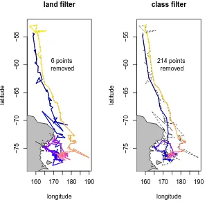
Figure 2.2: Land filter and Argos quality class filter. In the first panel any point occuring on land has been removed, and in the second any point with an Argos class of quality <“B” has been removed. In each panel the state of the track prior to filtering is shown as a dotted line. The coloured filtered line uses the same time-based colouring as in Figure 2.1.

track plotted in longitude and latitude coordinates.

In the first panel the original track has been filtered for points on the land area, and the second for points that have a location quality class of “B” or “Z”. The land filter only applies to six points in the track, but the class filter has removed 214, which is a majority of the available 351 points. The effects that these filters have are independent of one another and it would not matter which were performed before the other, although the result may be quite different in combination that in the use of either one alone.

In terms of the land mask, the filter succeeds in removing points from land but there is still a line segment that crosses a portion of the Antarctic continent. A filter that applies to points is quite different to one that applies to a continuous line segment. The class filter provides a track that seems more realistic than the noisy input track, but at the expense of discarding more than half of the available data.

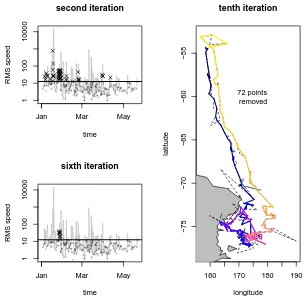
McConnell et al. (1992) to the Argos track. This technique specifies a running root-mean-square (RMS) summary of speed calculated by determining the instantaneous speeds for each point to each of its two previous and next locations. The RMS is defined as the square root of the mean of the speeds squared. Any sequence of locations with an RMS exceeding the maximum speed value have the peak RMS location discarded and the RMS is recalculated. This continues until all locations have an RMS less than the maximum speed. The threshold applied in this example is 12 km/h. Again the track is presented as longitude/latitude coordinates with distance measurements calculated relative to the WGS84 ellipsoid.

In the left panels of Figure 2.3 are two plots of the RMS values, for the second iteration after some positions are removed and the sixth iteration when only a few nearby positions remain above the threshold. The unfiltered RMS values are shown as a grey line representing the original points, the current points that have RMS values above the maximum are shown as crosses and the points below the maximum are shown in faded black. The threshold speed is shown as a horizontal line. As successive peaks of RMS values above the maximum are removed the categorization for the remaining points changes. This filter took ten iterations to remove all of the 73 locations that imply a speed of movement faster than the threshold, and the resulting track is shown in the right panel.

This result seems reasonable, though there is no end to the complexity and arbitrary nature of the decisions to be made. There are practical uses for techniques like these however. Speed filtering can give a reasonable result and there is a need to quantify the limits here with comparative studies of various algorithms on known data sets.

There are more sophisticated filtering algorithms that apply a suite of tests. A published speed-distance-angle filter first removes a minimum class (such as Z), filters for speed with the McConnell algorithm and then recursively removes further offending points that have a combination of acute angles and long implied distances travelled (Freitas et al., 2008). However, the accompanying software is quite specific and unrelated to other packages. In Section 2.4 a speed-distance-angle filter is defined completely using tools available in the trippackage.

Related filters applying a combination of metrics have been published by Douglas (2006), Croxall et al. (2004) and Austin et al. (2003). The algorithm published by Austin is available in the Rpackage DiveMove(Luque, 2007) and those by Freitas et al. (2008) and McConnell et al. (1992) inargosfilter. Freitas et al. (2008) gives an overview of the relative merits of various techniques, and the need for hierarchical techniques to avoid discarding good quality locations.

Another decision process is to choose between two possible locations for each time step provided by the Argos Service in the DIAG format (Service Argos, 2004). The Douglas Argos-Filter Algorithm applies this as part of the filter (Douglas, 2006).

2.3.2 Non-destructive filtering

Jan Mar May

1

10

100

10000

second iteration

time

RMS speed

Jan Mar May

1

10

100

10000

sixth iteration

time

RMS speed

160 170 180 190

−75

−70

−65

−60

−55

tenth iteration

longitude

latitude

72 points removed

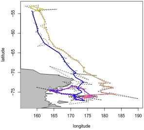
to modify light level geo-locations for latitude with SST (Beck and McMillan, 2002) and interpolative techniques to smooth tracks (Tremblay et al., 2006). Many de-structive filters can be recast in a non-dede-structive form using a penalty smoothing approach in the style of Green and Silverman (1994). For example, rather than filter the track to exclude locations that would imply an unrealistic speed of travel, the track can be smoothed using a speed of travel penalty. The smoothed locations are determined by minimizing the functional

Jλ(ˆx) = n

X

i=1

d(xi,xˆi)2+λ n−1 X

i=1

v(ˆxi, ti,xˆi+1, ti+1)2

where {x1, . . . , xn} represent the raw (unsmoothed) locations, {xˆ1, . . . ,xˆn} their

smoothed counterparts,d(x, y) represents the distance fromxtoy, andv(x, tx, y, ty)

the speed required to travel fromxat timetxtoyat timety, andλis the smoothing

parameter. The first term is a measure of goodness of fit of the smoothed locations ˆ

xi to the raw locations xi, while the second is a speed penalty. Minimizing Jλ

trades off goodness of fit against speed of travel. When λ= 0 the smoothed track reproduces the raw track exactly. Increasingλfavours tracks requiring less extreme speeds, at the expense of reproducing the xi.

As for the more traditional application described by Green and Silverman (1994) this process can be interpreted in a Bayesian context. Adopting a penalty based on squared speeds is equivalent to adopting a Gaussian prior on speeds, adopting a penalty based on the absolute values of speed is equivalent to an exponential prior on speed.

An application of this non-destructive filter was applied to the example Argos data set discussed earlier. Figure 2.4 shows the filtered result on a map and Fig-ure 2.5 shows the same result with longitude and latitude plotted against time. The result seems reasonable with a plausibility comparable to that of the recursive speed filter with the advantage of not having removed any data from the trip.

2.3.3 Spatial smoothing—surfaces from track data

There are a number of ways of creating bivariate (surface) estimates from track data, the most common involve a surface defined by a grid of cells or connected points. (Regular grids are historically easy to store and to compute, and so are applied most commonly—irregular grids and meshes are not considered here). The most direct methods are variously called “rasterization”, “gridding” or “pixellation”— these effectively generate a bivariate histogram from the input point or line data. Kernel methods apply a bivariate distribution (such as a Gaussian) to the input points or lines. Point methods are not discussed here, but can be achieved in a similar way to the line-based examples shown in Section 2.4.

160 165 170 175 180 185 190

−75

−70

−65

−60

−55

longitude

latitude

Jan Mar May

160

175

190

time

longitude

Jan Mar May

−75

−65

−55

time

latitude

of interest was pure residency—the minimal region in which the animal is present (home range) and the animal’s core region. In this context actual “tracks” are not the main interest. Marine applications have traditionally been explicitly interested in tracks and the temporal relationships, perhaps because of the real and perceived differences in the dynamics of marine environments. Modern techniques are seeing a far greater cross-over in these originally different fields and the differences are now out-weighed by the common goal of reliable location estimation.

Cell binning and kernel density estimation (KDE) can unproblematically con-vert a linear geometric track representation into a 2D histogram-like smoothing of residency, time spent map, or other utilization distribution but both must grapple with serious problems of interpretation. Points and lines simply do not represent the movement of an animal completely. Both methods must deal with issues of inde-pendence, point or line interpretations and complex boundaries and environmental relationships. If these issues can be dealt with or ignored, both cell gridding or KDE can be used as a convenient smoother for track data.

The following combinations of methods are applied in various ways in many existing publications (for example see Seaman et al. (1999); Wood et al. (2000); Nel et al. (2002); Bradshaw et al. (2002); Croxall et al. (2004)). The grid surface is generated by operating on points or on line segments. Line segments provide a continuity through space and so they provide a natural way to connect regions visited by the animal. Lines present a harder problem to convert to a grid than points and so this is often approximated by providing interpolated points in place of line segments, assuming constant travel speed.

The influence of the points or lines on the surface is calculated by binning into the overlapping grid cells directly, or by calculating the contribution to neighbour cells via a “kernel”. In the case of binning, the coverage provided by overlay with cells is relatively small, and completely dependent on the chosen bin size. This leads to compromises balancing positional accuracy and the need to match the scales of covariate data Bradshaw et al. (2002). These limitations are the same as those for histograms in general—the discontinuous histogram presents analytical difficulties as it quite senstive to the chosen origin, bin size and orientation (Simonoff, 1996; Silverman, 1998). Kernel density has the advantages that the result is smooth with-out the blocky, discontinuous nature of a bivariate histogram. Regular or irregular “wireframe” representations give a smoother result and have continuous analytical and visualization counterparts via interpolation, but these data structures are more complicated to calculate and are much less widely supported.

Finally, when the cell value is determined there are various ways in which the contribution of a point or line can be calculated. The point or line can simply be summed into the cell—a point is counted as present in the cell whereas the proportional length of an overlapping line segment is added to the bin. Each bin contribution can be multiplied by a factor, such as a point value or the time interval available to a line segment. This is one of the natural cases for using line segments from track data rather than points, as when the duration of time is of interest the input points cannot represent the duration of time. Many studies approximate this by creating a regular time series by interpolation.

ei-ther dimension of the kernel, or more generally a two-dimensional correlated weight-ing is used (Simonoff, 1996).

The following examples show the gridding of a very simple track by some different methods.

Exact gridding

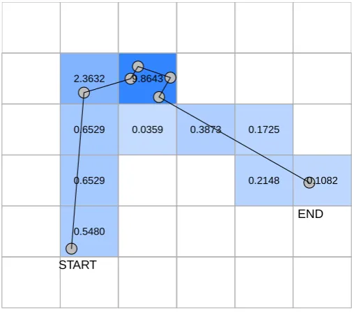
Gridding (pixellation or rasterization) methods generate a grid of cells that extend completely over the region of input track data.

A very simple track is shown in Figure 2.6 with an underlying grid. Each line segment has a value assigned to it, the time duration between each track point. These values are [2, 3, 1, 7, 1, 1] and the first and last line segments are quite long, so their contribution to the cells is small relative to the middle segments. This is reflected in the grid, which represents the implied “time spent” in each cell. In order to determine the contribution of each line segment’s value to a cell, the segment is split on the boundaries of the cells that it crosses and the value shared proportionally based on the length of the resulting segment-portion. This computation is not simple—to describe it in GIS terms this is an overlay of the line and the cells (“topology overlay”) with a rule to transfer values from the lines to the cell, in this case a proportional sum. GIS can be used to perform these calculations, but as discussed in Section 2.2.3 working with time in GIS is not well supported and this must be done as an attribute on line objects, rather than on inherently continuous lines that vary through time or other dimensions as well as space.

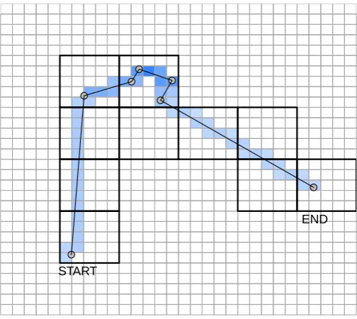
The dependence of the gridding method on bin size is easy to see. Figure 2.7 shows the same gridding process applied to a finer grid, with the same origin. The grid again completely summarizes the contribution of the track, but the actual regions influenced by the grid are quite different—the small grid cells snugly trace the track and cover a much smaller overall area than in the case of the coarse grid. The total time duration represented by the coarse and fine grid is exactly the same, but the results are quite different.

This dependence on scale has been used explicitly to provide a compromise between positional accuracy and spatial coverage with the need to match with envi-ronmental data by Bradshaw et al. (2002) and Burns et al. (2004). Bradshaw et al. (2002) also explicitly used grid size to help acccount for spatial uncertainty. As discussed previously the assumptions made by these analyses become substantial, involving issues such as uniform location accuracy, uniform grid scale and constant straight line travel.

Kernel density methods

●

● ●

● ● ●

●

2.3632 9.8643

0.6529 0.0359 0.3873 0.1725

0.6529 0.2148 0.1082

0.5480

START

END

● ●

● ●

●

●

●

START

END