Tableaux for Quantified Hybrid Logic
?Patrick Blackburn1and Maarten Marx2 1
INRIA, Lorraine, Nancy, [email protected]
2 ILLC, University of Amsterdam, the Netherlands.[email protected]
Abstract. We present a (sound and complete) tableau calculus for Quantified Hybrid Logic (QHL).QHLis an extension of orthodox quantified modal logic: as well as the usual2and 3modalities it contains names for (and variables over) states, operators@sfor asserting that a formula holds at a named state, and a binder↓that binds a variable to the current state. The first-order component contains equality and rigid and non-rigid designators. As far as we are aware, ours is the first tableau system forQHL.
Completeness is established via a variant of the standard translation to first-order logic. More concretely, a validQHL-sentence is translated into a valid first-order sentence in the correspondence language. As it is valid, there exists a first-order tableau proof for it. This tableau proof is then converted into aQHLtableau proof for the original sentence. In this way we recycle a well-known result (complete-ness of first-order logic) instead of a well-known proof.
The tableau calculus is highly flexible. We only present it for the constant domain semantics, but slight changes render it complete for varying, expanding or con-tracting domains. Moreover, completeness with respect to specific frame classes can be obtained simply by adding extra rules or axioms (this can be done for every first-order definable class of frames which is closed under and reflects generated subframes).
1
Introduction
Hybrid logic is an extension of modal logic in which it is possible to name states and to assert that a formula is true at a named state. Hybrid logic uses three fundamental tools to do this: nominals, satisfaction operators, and the↓-binder. Nominals are special propositional symbols that are true at precisely one state in any model: nominals ‘name’ the unique state they are true at. A satisfaction operator has the form@swheresis a
nominal. A formula of the form @sφasserts thatφis true at the state named by the
nominals. Finally, a formula of the form ↓s.φbinds all occurrences of the nominal sinφto the current state of evaluation — that is, it makessa name for the current state. (Actually, so that we don’t have to worry about accidental binding in the course of tableau proofs, we shall distinguish between ordinary nominals, which cannot be bound, and ‘state variables’ which are essentially bindable nominals.)
?
Hybrid logic has a lengthy history (see the web pagewww.hylo.netfor further information), and over the years it has become clear that adding the hybrid apparatus of nominals (and state variables), satisfaction operators, and↓to modal logic often results in systems with better logical properties than the original. But most previous work on hybrid logic has examined the effects of hybridizing propositional modal logics. What about quantified (first-order) hybrid logic?
In fact, strong evidence already exists that quantified hybrid logic (QHL) is also better behaved logically than orthodox quantified modal logic. In [2], the only recent paper devoted to the topic, it is shown that a very general interpolation theorem holds in QHL(as is well known interpolation almost never holds in orthodox quantified modal logic [3]). The purpose of the present paper is to show thatQHLis well behaved in another respect: just as in the propositional case, it is possible to define simple and intuitive tableau systems. We shall present a tableau system for QHLwhich handles equality, and rigid and non-rigid designators.
Our method for proving completeness is very simple and inspired by Jerry Selig-man’s paper [10]. Instead of redoing a proof we use existing results. Correspondence theory and its notion of a standard translationST(·)places the model theory of (propo-sitional and first-order) modal logic firmly into first-order logic [12, 13]. Our plan is the following. We prove completeness for our tableaux calculus by taking a proof P for
STφin a proven complete first-order calculus, and transformPinto a proofP0forφin our calculus. The tableaux system we use is by Fitting, in particular the one presented in [4]. This strategy works in hybrid logic because it has an equivalent expression for every subformula which might occur in a first-order proof of a translated formula.
Outline of paper. The paper starts with a definition of first-order hybrid logic. Then
we present the tableau system in three natural parts. The forth section is devoted to completeness issues. Again we split them up into three natural parts. This section ends with a very general completeness result. Finally we draw conclusions.
2
Quantified Hybrid Logic
We first define the syntax ofQHL. We have a setNOMof nominals, a setSVARof state variables, a setFVARof first-order variables, a setCONof first-order constants, a setIC
of unary function symbols, and predicates of any arity (note that predicates of nullary arity are simply propositional variables). The terms of the language are the constants fromCON, the first-order variables fromFVARand the terms generated by the rule
ifq∈ICands∈NOM∪SVAR, then@sqis a term.
(For readers familiar with propositional hybrid logic, this notation may come as a sur-prise: we are combining a satisfaction operator with a term to make a new term. But as the semantics defined below will show, overloading the@notation in this way is quite natural:@sqwill be the value of the non-rigid termqat the world named bys.)
The atomic formulas are all symbols inNOMandSVARtogether with the usual first-order atomic formulas generated from the predicate symbols and equality using the terms. Complex formulas are generated from these according to the rules
Herex∈FVAR,w∈SVARandn∈NOM∪SVAR.
These formulas are interpreted in first-order modal models with constant domains. AQHLmodel is a structure(W, R, D, Inom, Iw)w∈W such that
– (W, R)is a modal frame;
– Inomis a function assigning members ofW to nominals;
– for everyw∈W,(D, Iw)is an ordinary first-order model such that
• Iw(c) =Iw0(c), for allw, w0∈W and constantsc;
• Iw(q)∈D, forqa unary function symbol;
• Iw(P)⊆kD, forP ak-ary predicate symbol.
To interpret formulas with free variables we use special two-sorted assignments. AQHL
assignment is a functiongfromSVAR∪FVARtoW ∪Dwhich sends state variables to members of W and first-order variables to elements ofD. Given a model and an assignmentg, the interpretation of termst, denoted by¯t, is defined as
¯
x =g(x) forxa variable
¯
c =Iw(c) forca constant and somew∈W
@nq=
IInom(n)(q)ifna nominal Ig(n)(q) ifna state variable.
forqa unary function symbol
Formulas are now interpreted as usual. Withgx
d we denote the assignment which is just
likeg except thatg(x) = d.M, g, s φmeans thatφholds in model Mat states under the assignmentg. The inductive definition is
M, g, sP(t1, . . . , tn) ⇐⇒ ht¯1, . . . ,¯tni ∈Is(P)
M, g, sti=tj ⇐⇒ ¯ti = ¯tj
M, g, sn ⇐⇒ Inom(n) =s, forna nominal
M, g, sw ⇐⇒ g(w) =s, forwa state variable M, g, s¬φ ⇐⇒ M, g, s,6φ
M, g, sφ∧ψ ⇐⇒ M, g, sφandM, g, sψ M, g, sφ∨ψ ⇐⇒ M, g, sφorM, g, sψ M, g, sφ→ψ ⇐⇒ M, g, sφimpliesM, g, sψ M, g, s∃xφ ⇐⇒ M, gxd, sφ, for somed∈D M, g, s∀xφ ⇐⇒ M, gxd, sφ, for alld∈D
M, g, s3φ ⇐⇒ M, g, tφfor somet∈W such thatRst M, g, s2φ ⇐⇒ M, g, tφfor allt∈W such thatRst M, g, s@nφ ⇐⇒ M, g, Inom(n)φforna nominal
M, g, s@wφ ⇐⇒ M, g, g(w)φforwa state variable
M, g, s↓w.φ ⇐⇒ M, gw s, sφ.
3
The tableau calculus
1. A is complete for the propositional modal language expanded with nominals and @. (We name this systemHL(@); in the literature it is often called the basic hybrid
language.)
2. A∪Bis complete forHL(@,↓), the expansion ofHL(@)with state variables and the↓binder;
3. A∪B∪Cis complete forQHL.
Some terminology. As usual, a tableau branch is closed if it containsφand¬φ, whereφis a formula. A tableau is closed if each branch is closed. A branch is atomically
closed if it closes on an atom and its negation. A (tableau) proof of a hybrid sentence
φis a closed tableau beginning with¬@sφ, wheresis a nominal not occurring inφ.
3.1 Tableau forHL(@)
A key feature of our tableau is that all modal formulas occurring in a proof are grounded to a named world by their label. (This same feature also occurs in labelled tableau for propositional modal logic [8, 7].)
Grounding to a named state is implemented in our system by ensuring that all for-mulas occurring in proofs are of the form @sφor ¬@sφ for s a nominal. Thus the
propositional rules become
Conjunctive rules @s(φ∧ψ)
@sφ
¬@s(φ∨ψ)
¬@sφ
¬@s(φ→ψ)
@sφ
@sψ ¬@sψ ¬@sψ
Disjunctive rules @s(φ∨ψ)
@sφ | @sψ
¬@s(φ∧ψ)
¬@sφ | ¬@sψ
@s(φ→ψ)
¬@sφ | @sψ
Negation rules
¬@s¬φ
@sφ
@s¬φ
¬@sφ
To these we add rules for diamond and box. In the diamond rules,tis a nominal which does not occur on the branch.
Diamond rules @s3φ
@s3t
¬@s2φ
@s3t
@tφ ¬@tφ
Box rules @s2φ, @s3t
@tφ
¬@s3φ, @s3t
¬@tφ
Finally the rules for@. There are two rewrite rules to delete nestings of@. Next, as @streally means thatsandtare equal, there are rules to handle equality. These three
@ rules @s@tφ
@tφ
¬@s@tφ
¬@tφ
[son the branch] @ss
[Ref] @st @sϕ @tϕ
[Nom]@st @r3s @r3t
[Bridge]
The following rules can be derived: @st @ts
[Sym] @st @tr @sr
[Trans] @st @tϕ @sϕ
[Nom−1]
Example. Below we give a tableau proof for(3p∧3¬p) → (2(q → n) → 3¬q). Herenis a nominal andp, qare propositional variables. The formula expresses that if a state has two successors, then if it has at most oneqsuccessor, it has at least one¬q successor. Note that this is not expressible in ordinary modal logic. In ordinary modal logic we cannot put an upper bound on the number of successors.
1. ¬@s(3p∧3¬p→(2(q→n)→3¬q))
2. @s(3p∧3¬p)
3. ¬@s(2(q→n)→3¬q)
4. @s3p
5. @s3¬p
6. @s2(q→n)
7. ¬@s3¬q
8. @s3t
9. @tp
10.@s3r
11.@r¬p
12.@t(q→n)
13.1¬@tq 14.@tn
13.2¬@t¬q 15.@r(q→n)
13.3 @tq
16.1¬@rq 17.@rn
16.2¬@r¬q 18.@nr
16.3 @rq 19.@tr
20.@rp
21.¬@rp
In this, 2 and 3 are from 1 by a conjunctive rule; 4,5,6,7 are from 2 and 3 by conjunctive rules; 8,9,10,11 are from 4 and 5 by diamond rules; 12 is from 6 and 8 by box; 13.1 and 14 are from 12 by a disjunctive rule; 13.2 is from 7 and 8 by box; 13.3 is from 13.2 by a negation rule. The branch closes on 13.3 and 13.1.
15 is from 6 and 10 by box; 16.1 and 17 are from 15 by a disjunctive rule; 16.2 is from 10 and 7 by box; 16.3 is from 16.2 by a negation rule. The branch closes on 16.1 and 16.3.
3.2 Tableau forHL(↓,@)
To obtain a complete tableau system for the expansion ofHL(@)with variables over states and the binder↓, we only need to add the following two rewrite rules to the rules forHL(@):
Downarrow rules @s↓w.φ
@sφ[s/w]
¬@s↓w.φ
¬@sφ[s/w]
Here[s/w]means substitutesfor all free occurrences ofwinφ. Becausesis always a nominal, whence cannot be quantified over, we do not have to worry about accidental bindings. As an example the reader can try to prove the validities↓w.3w→(p→3p) and↓w.23w→(32p→p).
3.3 Tableau forQHL
A complete tableau system for quantified hybrid logic consists of theHL(↓,@)system, plus the (adjusted) rules for the quantifiers and equality from Fitting’s system (see [4]) for first-order logic with equality, plus two rules relating equalities across worlds. In the existential rules,cis a parameter which is new to the branch. As parameters are never quantified over, the substitution[c/x]is free for the formulaφ(x). In the universal rules, tis any grounded term on the branch (thus either a first-order constant, a parameter or a grounded definite description). A grounded definite description is a term@nqforna
nominal andqa non-rigid designator fromIC.
Existential rules @s∃xφ(x)
@sφ(c)
¬@s∀xφ(x)
¬@sφ(c)
Universal rules @s∀xφ(x)
@sφ(t)
¬@s∃xφ(x)
¬@sφ(t)
Besides Fitting’s [4] Reflexivity (Ref) and Replacement (RR) rules, there are three extra rules for equality. The first (called DD) states that ifnandmdenote the same state, then@nqand@mqdenote the same individual. The second and third (both called
@=) embody that equality is a rigid predicate: if two terms are the same in one world, they are the same in every world. Because these two rules peel the leading@n from
equalities, reflexivity and replacement can be kept in the old format. In the Replacement rule,φ[u]denotesφ(t)with some of the occurrences oftreplaced byu.
QHLEquality rules
t=t[Ref]
t=u, φ(t) φ[u] [RR],
@nm
@nq= @mq
[DD] @n(ti=tj) ti=tj
[@=] ¬@n(ti=tj)
¬(ti=tj)
Example. The most interesting examples deal with equality and rigid and non-rigid
designators. Consider the sentence Caroline is Miss America. When formalising this let cbe a rigid designator denoting Caroline and qa non-rigid designator denoting Miss America. Then↓x.(c= @xq)means Caroline is the present Miss America. It is true in
a statewifIw(c) =Iw(q). This formula has the following relation with the2operator:
6|= (↓w.c= @wq)→2↓w.c= @wq
(1)
|= (↓w.c= @wq)→ ↓w.2c= @wq.
(2)
A falsifying model for the sentence in (1) is given by two worldsnandm, withRnm, and a domain{a, b}with the interpretationIn(c) =Im(c) =In(q) =aandIm(q) =b.
Then (1) fails at world n. When downarrow has wide scope in the consequent, the formula becomes true. Here is the tableau proof:
1.¬@n((↓w.c= @wq)→ ↓w.2(c= @wq))
2.@n↓w.c= @wq
3.¬@n↓w.2(c= @wq)
4.@n(c= @nq)
5.¬@n2(c= @nq)
6.@n3m
7.¬@m(c= @nq)
8. c= @nq
9.¬(c= @nq).
In this, 2 and 3 are from 1 by a conjunctive rule; 4 and 5 are from 2 and 3 by a downarrow rule, respectively; 6 and 7 are from 5 by a diamond rule; 8 and 9 are from 4 and 7 by an @= rule, respectively.
4
Soundness and Completeness
The argument to establish soundness follows the familiar pattern: show that satisfia-bility is preserved by each tableau rule application. This is easy to check and left to the reader. Completeness will be established using the standard translation and a com-plete first-order inference system. We use the system that is closest to the one presented here: the tableau calculus for first-order logic with equality from Fitting [4] with the reflexivity and replacement rules (restricted to atoms). The main line of the argument is the following. We need to establish that every validQHLsentence has aQHLtableau proof. The standard translation preserves validity, thus aQHL sentenceφ is valid if and only if the first-order sentenceSTφis valid. For validSTφ, there exists a closed first-order tableau proof T starting with¬ST φ. Our task is to transform this closed first-order proofT starting with¬STφ into a closed QHLtableau proof T0 starting with¬φ.
Before we can continue we have to settle two things. We change Fitting’s first-order tableau rules a little bit in order to better cope with translations of modal formulas. Besides that we have to use a modified translation. We start with the former.
In order to save on inductive proofs and definitions, we assume from now on that theQHLlanguage contains as primitive logical operators only¬,∧,2,@s,↓w.and∀v.
Clearly this is without loss of generality because the other operators can be defined in terms of these.
4.1 Tableau rules for relativized quantifiers
The translation of a box modality yields a relativized universal formula of the form
∀x(A(x) → C(x)), withA(x)an atom. For these relativized universals, a more effi-cient tableau rule exists than the combination of universal and→rule together. In fact it is nothing but Modes Ponens. Forta closed term,
Modes Ponens (MP) A(t), ∀x(A(x)→φ(x))
φ(t)
A(t), ¬∃x(A(x)∧φ(x))
¬φ(t)
We change Fitting’s calculus such that on universals relativized by an atom the normal universal rules cannot be applied, but MP can. This is easily seen to be complete (cf., also [11]). We can make a further reduction in complexity in the case the antecedent is an equality. Then the statement just expresses a substitution. We also add the following rules to Fitting’s calculus and make the proviso that universal and existential rules are never applied to quantified sentences relativized by an equality.
Substitution Rules
∀x(x=t→φ(x)) φ(t)
∃x(x=t∧φ(x)) φ(t)
¬∀x(x=t→φ(x))
¬φ(t)
¬∃x(x=t∧φ(x))
¬φ(t)
4.2 Translation using predicate abstraction
Unfortunately, the standard translation does not square well with the intention to change one proof into another because it does not preserve syntactic structure. Because we want to transform a proof for the translation ofφinto a proof forφ, we need to translate backwards as well. It is crucial that applying the backwards translation to the translation ofφyieldsφagain. This is simply not obtainable by the standard translation or obvious variants.
An example might explain why not. We can read@s(p∧q)as saying that states
has the propertyp∧q. As we want to translate proposition letters to one place predi-cates, in first-order logic we can only say then thatshas property p andshas property q. This is of course logically equivalent, but syntactically different. We would like to have machinery which can turn formulas into predicates, so that we can speak about the property “pandq”. The lambda calculus provides precisely this:hλx.(P x∧Qx)i
We work in first-order logic with predicate abstraction restricted to variables ranging over individuals. Thus we only add a piece of syntactic sugar. The expressive power of the language remains the same, it is just first-order logic. For a thorough introduction to real predicate abstraction in modal logic we refer to [6].
Supposeφis a first-order formula andxa first-order variable. Then hλx.φiis a predicate abstract. Its free variable occurrences are the free variable occurrences of φ except for x. Predicate abstracts behave as unary predicate symbols; new atomic formulas from predicate abstractshλx.φican be made by the rule
iftis a term, thenhλx.φi(t)is a formula.
Examples arehλx.P xi(t)andhλx.P x∧Qxi(s). The new formulas get their meaning by performingβ-reduction:
theβ-reduction ofhλx.φi(t)isφ[t/x].
The meaning ofhλx.φi(t)is simply the meaning ofφ[t/x]. This shows that the expres-sive power remains the same. Our convention is that inλexpressions, the.takes wide scope, thushλx.φ∧ψi=hλx.(φ∧ψ)i.
In order to handle predicate abstracts in tableau proofs, we need only add two very simple rules to Fitting’s system. The rules just implementβ-reduction. Here they are
Abstract rules
hλx.φi(t) φ[t/x]
¬hλx.φi(t)
¬φ[t/x]
Fitting’s tableau system with the two abstract rules added is a complete inference system for the expansion of first-order logic withλ abstraction with variables ranging over individuals [5].
We are ready to define the new standard translation AT for the propositional hybrid language, together with its inverse AT−. In a certain sense, this translation can be traced back to the paper [9] in which McCarthy and Hayes introduce the situation calculus. ATy(φ)andAT−y(φ)are defined in the same way but withxandyinterchanged, e.g.,
ATy(p) :=P yandATy(2φ) :=hλy.∀x(Ryx→ATx(φ))i(y).
ATx(p) := P x
ATx(n) := x=n
ATx(¬φ) := hλx.¬ATx(φ)i(x)
ATx(φ∧ψ) := hλx.ATx(φ)∧ATx(ψ)i(x)
ATx(2φ) := hλx.∀y(Rxy→ATy(φ))i(x)
ATx(@nφ) := hλx.∀x(x=n→ATx(φ))i(x)
AT−x(P x) := p AT−x(x=n) := n
AT−x(hλx.¬φi(x)) := ¬AT−x(φ)
AT−x(hλx.φ∧ψi(x)) := AT−x(φ)∧AT−x(ψ) AT−x(hλx.∀y(Rxy→φ)i(x)) := 2AT−y(φ)
The following properties ofAT andAT−hold, for everyHL(@)formulaφ,
ATx(φ)is always a formula of the formhλx.ψi(x)orP xorx=n.
(3)
AT−x(ATx(φ)) =φ, and similarly whenxis replaced byy.
(4)
φisHL(@)valid iffATx(φ)is first-order valid.
(5)
(3) follows from the definition. (4) is proved by induction on the complexity of the
HL(@)formula. (5) is immediate by performingβ-reduction and the well-known result on the standard translation.
4.3 Completeness forHL(@)
Theorem 1. TheHL(@)tableau calculus is complete.
We now specify an algorithm for turning a closed Fitting tableau for the formulaATx(φ)[c/x]
(wherecis a parameter) into a closedHL(@)tableau for@cφ. Some terminology will
be useful. A literal is a grounded formula of the form
P(t)|t=u|Rtu| hλx.φi(t)| hλy.φi(t), or its negation.
Define the following translation(·)∗from positive literals toHL(@)sentences
P(t)∗ := @tp
(t=u)∗ := @tu
(Rtu)∗ := @t3u
(hλx.φi(t))∗ := @tAT−x(hλx.φi(x))
(hλy.φi(t))∗ := @
tAT−y(hλy.φi(y)).
For negative literals(¬φ), we set(¬φ)∗=¬φ∗.
We recapitulate:ATtranslates a hybrid formula into a first-order formula andAT− translates them backwards. The translation(·)∗ translates literals occurring in a first-order tableau proof into hybrid formulas. Note that these literals may contain parameters introduced in the proof. The crucial connection between the forward and backward translations is that they preserve syntactic structure: for φa hybrid formula and t a nominal or parameter,
(ATx(φ)[t/x])∗= @tφand(¬ATx(φ)[t/x])∗=¬@tφ.
(6)
Property (6) follows immediately from the definition of(·)∗and (4).
We are ready to specify the algorithm. LetTbe a closed Fitting tableau for the formula ATx(φ)[c/x]. Without loss of generality we may assume thatT is atomically closed.
LetT0 simply beT with all literals replaced by their(·)∗translation and all other for-mulas removed.
Claim T0isHL(@)tableau proof forφ.
We first observe that T0 starts with ¬@cφ. This is because T starts with the literal
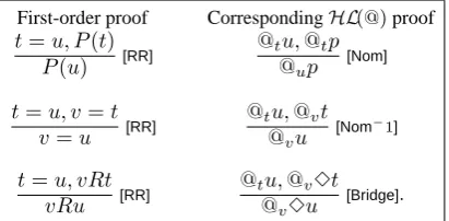
First-order proof CorrespondingHL(@)proof t=u, P(t)
P(u) [RR]
@tu,@tp
@up
[Nom]
t=u, v=t v=u [RR]
@tu,@vt
@vu
[Nom−1] t=u, vRt
vRu [RR]
@tu,@v3t
[image:11.595.206.412.116.217.2]@v3u
[Bridge].
Table 1. Corresponding replacement proofs
Secondly, every branch inT0 closes. This is becauseT branches close on literals, which we all move over toT0, keeping the negation signs in place. We now show thatT0 is a correctHL(@)tableau, i.e. that every formulal∗inT0is derived from¬@cφby a
finite number ofHL(@)rule applications. We prove by induction on the structure of the literals that for all literalsl, l0inT, for all literalsl1, l2produced froml, l0by applying rules, the literalsl∗1, l∗2can be obtained froml∗, l0∗by applying a (derived) rule inT0.
There is only one zero premise rule. Ref can introduce literalst=tin T, which can be matched by the hybrid Ref rule producing(t=t)∗= @tt.
On literals which are notλ-formulas we can only perform Replacement, which we handle later. Every literal inTwhich is aλ-formula has the formhλz.ATz(ψ)i(t), for
zeitherxory, andψanHL(@)formula. Its(·)∗translation is@tψby (6). This gives
us with the cases presented in Table 2. This table is read as follows. On the left are first-order proofs with annotations indicating which rule is applied on what to obtain the result. On the right are theHL(@)proofs which derive the(·)∗ translated results from the(·)∗translated premises, again annotated.
We assumed Replacement only works on positive literals. The possible instantia-tions of literals in whichtis replaced are
t=v, v=t, vRt, tRv, P(t)andhλz.φi(t).
In Table 1 the application of the replacement rule is given on the left while the corre-spondingHL(@)proof on the(·)∗images of the formulas is on the right. As the cases forP(t),t=v,tRvandhλz.φi(t)are all by applications of Nom, we only show the case forP(t).
We considered all possible applications of all rules on all possible literals. ThusT0 is aHL(@)tableau.
4.4 Completeness forHL(↓,@)
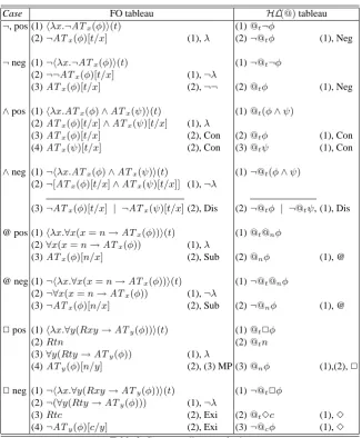
Case FO tableau HL(@)tableau ¬, pos (1)hλx.¬ATx(φ)i(t) (1)@t¬φ
(2)¬ATx(φ)[t/x] (1),λ (2)¬@tφ (1), Neg
¬neg (1)¬hλx.¬ATx(φ)i(t) (1)¬@t¬φ
(2)¬¬ATx(φ)[t/x] (1),¬λ
(3)ATx(φ)[t/x] (2),¬¬ (2)@tφ (1), Neg
∧pos (1)hλx.ATx(φ)∧ATx(ψ)i(t) (1)@t(φ∧ψ) (2)ATx(φ)[t/x]∧ATx(ψ)[t/x] (1),λ
(3)ATx(φ)[t/x] (2), Con (2)@tφ (1), Con (4)ATx(ψ)[t/x] (2), Con (3)@tψ (1), Con
∧neg (1)¬hλx.ATx(φ)∧ATx(ψ)i(t) (1)¬@t(φ∧ψ) (2)¬[ATx(φ)[t/x]∧ATx(ψ)[t/x]] (1),¬λ
(3)¬ATx(φ)[t/x] | ¬ATx(ψ)[t/x](2), Dis (2)¬@tφ | ¬@tψ, (1), Dis
@ pos (1)hλx.∀x(x=n→ATx(φ))i(t) (1)@t@nφ
(2)∀x(x=n→ATx(φ)) (1),λ
(3)ATx(φ)[n/x] (2), Sub (2)@nφ (1), @
@ neg (1)¬hλx.∀x(x=n→ATx(φ))i(t) (1)¬@t@nφ
(2)¬∀x(x=n→ATx(φ)) (1),¬λ
(3)¬ATx(φ)[n/x] (2), Sub (2)¬@nφ (1), @
2pos (1)hλx.∀y(Rxy→ATy(φ))i(t) (1)@t2φ
(2)Rtn (2)@tn
(3)∀y(Rty→ATy(φ)) (1),λ
(4)ATy(φ)[n/y] (2), (3) MP (3)@nφ (1),(2),2
2neg (1)¬hλx.∀y(Rxy→ATy(φ))i(t) (1)¬@t2φ
(2)¬(∀y(Rty→ATy(φ))) (1),¬λ
(3)Rtc (2), Exi (2)@t3c (1),3 (4)¬ATy(φ)[c/y] (2), Exi (3)¬@cφ (1),3
Table 2. Corresponding proof rules
With all the groundwork done, the proof is very easy. We have to extend the transla-tion to incorporate the variables and downarrow formulas. We assume thatxandyare new variables. The translation and its inverse for the state variables and downarrow is simply
ATx(w) := x=w
AT−x(x=w) := w
ATx(↓w.φ) := hλx.∀w(w=x→ATx(φ))i(x)
AT−x(hλx.∀w(w=x→φ)i(x)) := ↓w.AT−x(φ).
[image:12.595.145.472.111.506.2]4.5 Completeness forQHL
Theorem 3. The tableau system forQHLis complete.
Again the proof is simple after we made the needed straightforward adjustments. The translation and its inverse for the fullQHLlanguage is obtained by adding the following rules to the ones already existing:
ATx(P(t1, . . . , tk)) := P0(x, t1, . . . , tk)
ATx(ti=tj) := hλx.ti =tji(x)
ATx(∀vφ) := hλx.∀vATx(φ)i(x)
AT−x(P0(x, t1, . . . , tk)) := P(t1, . . . , tk)
AT−x(hλx.ti=tji(x)) := ti=tj
AT−x(hλx.∀vφi(x)) := ∀vAT−x(φ)
The translation(·)∗is extended for the new literals as follows:
P0(s, t1, . . . , tk)∗ := @sP(t1, . . . , tn)
(ti=tj)∗ := ti=tj.
We don’t translate theQHLterms@sqbut just pretend they are first-order termsq(s).
Again, properties (3)–(6) still hold. (The first-order tableau calculus has to respect the two sorts of course. For example, ∀xP0(s, x) does not yield the not correctly typed P0(s, s) by universal instantiation.) The atomic hybrid formulati = tj is translated
as hλx.ti = tji(x). This is done to have a syntactic analogue of @s(ti = tj). In a
first-order proof,β-reduction can be applied tohλx.ti=tji(s)or its negation, yielding
ti=tjand¬ti=tj, respectively. This proof step corresponds to an application of one
of the@ =rules on the(·)∗translations in aQHLtableau.
It is immediate that the quantifier rules can be mimicked inQHLtableaux (provided they respect the sorts).
For the application of replacement, there are now terms@nqforqa non-rigid
des-ignator andna nominal. The replacement rule in a first-order proof can then with the premisen=mreplace@nqby@mqin any atom. Butn=mback-translates to@nm
and from that theQHLequality rule DD yields@nq= @mq. Now replacement inQHL
with this premise on the translated atom yields the translated result.
Thus all first-order rules have a correspondingQHLanalogue and we are done.
4.6 Completeness for specific frame classes
disjoint unions. Closure under and reflection of generated subframes is a requirement which reflects the local evaluation of modal formulas.1
We recall from [1], that every such elementary class of frames is definable by a first-order sentence∀yγ(y), in whichγ(y)is equivalent to a pure hybridHL(@,↓)sentence γ0 (i.e., without propositional variables nor nominals). AsAT preserves meaning we may without loss of generality assume thatγ(y) =ATy(γ0).
Let such a classKbe defined by∀yγ(y). Then aQHLsentenceφis valid onKiff
∀yγ(y)→ATx(φ)[c/x]forca new parameter is first-order valid. In that case, there is
a first-order tableau proof starting with
1.∀yγ(y)
2.¬ATx(φ)[c/x].
Whence the proof will develop almost as for ATx(φ)[c/x] except that for any state
parameter or nominals,γ(s)may be introduced on the branch. This insight leads to the following rule to be added to theQHLtableau system:
@sγ0
forson the branch.
Now every time aγ(s)is added to the branch in the first-order proof, we apply the new rule onsin theQHLproof. Because of the assumption on the form ofγ, translating γ(s)by(·)∗yields@sγ0. Thus we have shown
Theorem 4. Letγa pure nominal free hybrid sentence which axiomatises the class of framesK. Then adding the above rule to theQHLtableau calculus yields completeness for the quantified hybrid logic of the class of framesK.
1
Added in proof. Balder ten Cate together with the first author of the present paper (from now on referred to as BC) have proposed a proof system forHL(@)which is complete for frame classes defined by formulas of the form∀x¯∃yφ¯ (¯x,¯y), in whichφis anHL(@)formula starting with@x1and the quantifiers bind all nominalsx¯andy¯occurring inφ. A natural example is
∀x1x2x3∃y@x1(@x13x2∧@x13x3 →@x23y∧@x33y)defining the class of confluent
frames.
BC claim that adding the rule (*) below to theHL(@)tableaux calculus given here is com-plete for the class of frames defined by∀x¯∃yφ¯ (¯x,y¯). This result is most easily proved using the developed theory of translations, as follows: Assume aHL(@)formulaψis valid on the class of frames defined by∀x¯∃yφ¯ (¯x,y¯). Then∀x¯∃yAT¯ x1(φ(¯x,y¯)) → ATx(ψ)[c/x]for
ca new parameter is FO valid. Thus there is a first-order tableau proof of it starting with ∀x¯∃yAT¯ x1(φ(¯x,y¯)),¬ATx(ψ)[c/x]. Our goal is to turn this tableau into anHL(@)tableau
as before. The only new thing we have to mimic is an application of universal instantiation followed by existential elimination to∀x¯∃yAT¯ x1(φ(¯x,y¯)). This is exactly what rule (*) of
BC is doing.
(∗)φ(¯s,t¯) fors¯nominals on the branch and all¯tnominals new to the branch.
5
Conclusions
The positive effects of hybridization in propositional logic extend well to the first-order case. In fact, one could argue that the need for hybridization is felt much stronger in first-order modal logic. The field is plagued with failures of desirable properties, and consequently more difficult and obscure than its propositional counterpart. Here we have presented an extremely general completeness theorem (Theorem 4) covering vir-tually all modally interesting elementary frame classes. In a companion paper we have shown that the calculus can be used to construct interpolants. Interpolation is one of the properties which fail in many quantified modal logics. This theorem also extends to all frame classes from Theorem 4. These very general results indicate that the additions to the syntax are natural and extremely useful.
The paper contained two important ideas. First and foremost is the proof method for showing completeness. An almost standard translation was used in a non-trivial way to transfer a first-order result into the modal setting. In the hybrid language, this was par-ticularly easy, as it contains such first-order proof-elements as parameters. In orthodox modal logic, too many completeness proofs are repeated with only tiny changes. Maybe hybridization is needed to change modal logic into a field in which standard results are recycled instead of proofs. It’s worth the price.
The second idea is our treatment of definite descriptions like Miss America.InQHL it is not possible to write intensional terms as in Montague’s IL. The hidden variables in intensional terms cause many technical problems and make IL mathematically com-plicated. The use of @ to ground non-rigid designators to states is a simple remedy.
References
1. C. Areces, P. Blackburn, and M. Marx. Hybrid logics: Characterization, interpolation and complexity. Journal of Symbolic Logic, 66(3):977–1010, 2001.
2. C. Areces, P. Blackburn, and M. Marx. Repairing the interpolation lemma in quantified modal logic. Report PP–2001–19, ILLC. To appear in Annals of Pure and Applied Logic. 3. K. Fine. Failures of the interpolation lemma in quantified modal logic. Journal of Symbolic
Logic, 44(2):201–206, 1979.
4. M. Fitting. First Order Logic and Automated Theorem Proving (second edition). Springer Verlag, 1996.
5. M. Fitting. Types, Tableaus, and G¨odel’s God. Unpublished Draft, 1999. 6. M. Fitting and R. Mendelsohn. First–Order Modal Logic. Kluwer, 1998. 7. D. Gabbay. Labelled Deductive Systems. Oxford University Press, 1996.
8. R. Gor´e. Tableau methods for modal and temporal logics. In M D’Agostino,et al editors,
Handbook of Tableau Methods, pages 297–396. Kluwer Academic Publishers, 1999.
9. John McCarthy and Patrick J. Hayes. Some philosophical problems from the standpoint of artificial intelligence. In B. Meltzer and D. Michie, editors, Machine Intelligence 4, pages 463–502. Edinburgh University Press, 1969.
10. J. Seligman. Internalization: The case of hybrid logic. Journal of Logic and Computation, 11(5):671–689, 2001.
11. R. Smullyan. First Order Logic. Springer–Verlag, 1968.
12. J. van Benthem. Modal Logic and Classical Logic. Bibliopolis, Naples, 1983.
13. J. van Benthem. Correspondence theory. In D.M. Gabbay and F. Guenther, editors,
References
1. C. Areces, P. Blackburn, and M. Marx. Hybrid logics: Characterization, interpolation and complexity. Journal of Symbolic Logic, 66(3):977–1010, 2001.
2. C. Areces, P. Blackburn, and M. Marx. Repairing the interpolation lemma in quantified modal logic. Technical Report PP–2001–19, Institute for Logic, Language and Computation, University of Amsterdam, 2001. To appear in Annals of Pure and Applied Logic.
3. K. Fine. Failures of the interpolation lemma in quantified modal logic. Journal of Symbolic
Logic, 44(2):201–206, 1979.
4. M. Fitting. First Order Logic and Automated Theorem Proving (second edition). Springer Verlag, 1996.
5. M. Fitting. Types, Tableaus, and G¨odel’s God. Unpublished Draft, 1999.
6. M. Fitting and R. Mendelsohn. First–Order Modal Logic. Kluwer Academic Publishers, 1998.
7. D. Gabbay. Labelled Deductive Systems. Number 33 in Oxford logic guides. Oxford Uni-versity Press, 1996.
8. R. Gor´e. Tableau methods for modal and temporal logics. In M D’Agostino, D Gabbay, R Haenle, and J Posegga, editors, Handbook of Tableau Methods, pages 297–396. Kluwer Academic Publishers, 1999.
9. John McCarthy and Patrick J. Hayes. Some philosophical problems from the stand-point of artificial intelligence. In B. Meltzer and D. Michie, editors, Machine
In-telligence 4, pages 463–502. Edinburgh University Press, 1969.
http://www-formal.stanford.edu/jmc/mcchay69.html.
10. J. Seligman. Internalization: The case of hybrid logic. Journal of Logic and Computation, 11(5):671–689, 2001.
11. R. Smullyan. First Order Logic. Springer–Verlag, 1968.
12. J. van Benthem. Modal Logic and Classical Logic. Bibliopolis, Naples, 1983.
13. J. van Benthem. Correspondence theory. In D.M. Gabbay and F. Guenther, editors,