Assessing the performance of horizontal axis marine current turbines : the impact of evaluation methods and inflow parameters

(1)

Assessing the Performance of Horizontal Axis

Marine Current Turbines: The Impact of

Evaluation Methods and Inflow Parameters

by

Masoud Rahimian, B.E., M.E

National Centre for Maritime Engineering and Hydrodynamics

Australian Maritime College

Submitted in fulfilment of the requirements for the degree of Doctor of Philosophy

(2)

ii

Declarations

I declare that ‘This thesis contains no material which has been accepted for a degree or

diploma by the University or any other institution, except by way of background information

and duly acknowledged in the thesis, and to the best of my knowledge and belief no material

previously published or written by another person except where due acknowledgement is made in the text of the thesis, nor does the thesis contain any material that infringes copyright.’

This thesis may be made available for loan and limited copying in accordance with the Copyright Act 1968

Signed:

Masoud Rahimian

(3)

iii

Statement of Published Work Contained in Thesis

The publishers of the papers comprising Chapters 2 to 4 hold the copyright for that content,

and access to the material should be sought from the respective journals. The remaining

non-published content of the thesis, Chapter 5, are submitted and under review, and may be made

available for loan and limited copying and communication in accordance with the Copyright

Act 1968.

Statement of Co-Authorship

The following people and institutions contributed to the publication of work undertaken as part

of this thesis:

 Masoud Rahimian, University of Tasmania (Candidate)

 Doctor Jessica Walker, Primary Supervisor, University of Tasmania (Author 1)

 Associate Professor Irene Penesis, Co-Supervisor, University of Tasmania (Author 2)

 Michael Sos, University of Tasmania (Author 3)

 Luke Johnston, University of Tasmania (Author 4)

Author details and their roles:

Paper 1: Rahimian M, Walker J, Penesis I. Numerical assessment of a horizontal axis marine current turbine performance. International Journal of Marine Energy. 2017;20: 151-64.

Chapter 2 was based on this paper. The Candidate was the primary author. Author 1 and Author

2 assisted with research direction, advice, and presentation. [Candidate: 80%, Author 1: 10%,

(4)

iv

Paper 2: Rahimian M, Walker J, Penesis I. Performance of a horizontal axis marine

current turbine– A comprehensive evaluation using experimental, numerical, and

theoretical approaches. Energy. 2018; 148:965-76.

Chapter 3 and parts of Chapter 4 were based on this paper. The Candidate was the primary

author. Author 1 and Author 2 assisted with research direction, advice, and presentation.

[Candidate: 80%, Author 1: 10%, Author 2: 10%].

Paper 3: Rahimian M, Walker J, Penesis I. The influence of shear flow and waves on the performance characteristics of a horizontal axis marine current turbine. Journal of Applied Energy. 2018. (submitted for review)

Chapter 5 is based on this paper. The Candidate was the primary author. Author 1 and Author

2 assisted with research direction, advice, and presentation. [Candidate: 80%, Author 1: 10%,

Author 2: 10%].

Paper 4: Sos M, Johnston L, Walker J, Rahimian M. The impact of waves and immersion depth on horizontal axis tidal turbine performance. 12th European Wave and Tidal Energy Conference (EWTEC2017). Cork, Ireland. p. 1-8.

This conference paper is included in the appendix. Author 3 and Author 4 completed the

experimental work presented in the paper and contributed to the drafting of the paper. Author

1 contributed to the conception and design of the project, the analysis and interpretation of the

research data, and prepared the paper. The Candidate contributed to the conception and design

of the project and the analysis and interpretation of the research data. [Author 3: 35%, Author

(5)

v

We the undersigned agree with the above stated proportion of work undertaken for each of the

published (or submitted) peer-reviewed manuscripts contributing to this thesis.

Signed:

Dr Jessica Walker Primary Supervisor

National Centre for Maritime Engineering and Hydrodynamics Australian Maritime College

University of Tasmania

Date: 02 May 2018

Assoc/Prof Irene Penesis Co-Supervisor

Date: 02 May 2018

Assoc/Prof Michael Woodward Director

(6)

vi

Acknowledgements

Finally, this wonderful chapter of my life has come to an end. It has been filled with joy and

tribulations, and I certainly was not able to make it through on my own.

Firstly, I would like to express my sincere gratitude to my supervisory team, Dr Jessica Walker

and Assoc/Prof Irene Penesis for their continuous support, patience, encouragement, and

immense knowledge. They have been great supervisors as well as tremendous mentors for me.

It has been a pleasure to work with them and I hope I can pass on what I have learnt from them.

My genuine thanks also goes to Dr. Zhi Leong, and Dr. Philip Marsh for sharing their CFD

knowledge, which helped me make through CFD difficulties. Special thanks must also go to

Rowan Frost, Jock Ferguson, and Tim Lilienthal for their technical support in the setup and

execution of experimental works.

I would like to express my appreciation to the turbine research team led by Prof Karen Flack

at the United States Naval Academy for sharing their rotor design, which was used as the basis

for the AMC turbine.

Last but not the least, thanks to Zhinous, my love, who brought colours into my life. This work

(7)

vii

Abstract

The oceans offer a considerable sustainable energy resource in the form of wave, marine currents and thermal energy and provide a potential alternative to fossil fuels. Marine current,

or tidal, energy can be harnessed using horizontal axis marine current turbines (HAMCTs). In

this work, the performance of a 2-bladed HAMCT was extensively investigated using

experimental, theoretical and numerical models under different flow conditions. The

motivation behind the study was to assess the influence of various parameters, associated with

an evaluation method and those involved in the environment of a deployment site, on turbine

performance. The employed evaluation methods were compared to find the best practice for

performance assessment in various operational conditions.

For this purpose, two physical scale models with diameters of 500 mm and 800 mm were

tested in the Australian Maritime College Towing Tank and Circulating Water Channel

(CWC). Towing tank results from the United States Naval Academy were also employed for

facility comparison as well as CFD model verification. The experimental results provide the

hydrodynamic characteristics of the turbine under the different inflow conditions in each

facility. The difference between the performances of the two scale models was found to be

mainly due to the effect of Reynolds number and possibly attributed to the blockage effect. To

predict the performance of a full-scale turbine, experiments on a scale model in conditions with

Reynolds number independency, in this study Re > 2×105_{, in a facility with little blockage is}

suggested. Unlike the towing tanks, the CWC did not have a uniform inflow. Using the

equivalent flow velocity, obtained from kinetic energy flux over the rotor swept area, in

dimensional analysis of the CWC data resulted in a better correlation with the towing tank

results. It shows that although the shear flow profile practically has little effect on the mean

power output per se, selecting the flow velocity by which the performance is analysed is

essential in scale model tests. The impact of facility bias on the performance assessment

appeared to be induced mainly from blockage and partially from the flow velocity profile.

An experimentally validated Blade Element Momentum (BEM) model was modified to

consider shear flow profile and Reynolds number in the performance calculations. In addition,

QBlade software was employed as a tool to investigate the effect of using local Reynolds

number over the blade span. No significant changes were seen in the BEM model results by

(8)

viii

showed that using local sectional Reynolds numbers in the prediction may be not worth the

effort to achieve results that were slightly more accurate than the model with a single reference

Reynolds number. BEM theory provides reasonable performance predictions for turbines in

steady flow conditions.

To establish detailed hydrodynamic characteristics of the turbine in ideal flow conditions,

an experimentally validated numerical model using Computational Fluid Dynamics (CFD) was

developed. Different CFD approaches were applied to the model to find the best numerical

practice for the performance evaluation of HAMCTs. The CFD model was modified to account

for sheared inflow and surface waves using volume of fluid (VOF) and single-phase methods.

A steady moving reference frame (MRF) simulation of the whole turbine model using the k-ω

SST turbulence model with the wall-function model was found to be the best approach for the

performance prediction of HAMCTs under steady inflow conditions in a balance between

simulation time and result accuracy. Conversely, a transient solution with the sliding mesh

method provided a better fit to the experimental results for turbine under waves and sheared

inflow velocity profiles. The CFD simulations showed that a sheared inflow velocity profile

had a cyclic effect on the blade loadings and almost no significant effect on the mean power

production of the turbine. The effect of turbine depth and waves on the mean power yield was

also negligible when the tip immersion depth of the turbine was more than half the turbine

radius. Since both wave and sheared flow velocity affect the quality of power output even in

deeper positions, they should be considered during the turbine design stage. Regardless the

angular position of the blades, the maximum values of CPand CToccurred at the passing wave peaks and the minimum values at the troughs.

This study comprehensively evaluated the methods available to predict the performance of

HAMCTs and provided a detailed discussion of the different parameters that affect both turbine

and model performance. Overall, the BEM model provided accurate performance results in the

steady flow condition, though it was unable to capture the effect of shear velocity on the turbine

hydrodynamics. The QBlade model yielded similar results to the BEM model with the possibility of investigating Reynolds number effect; a user-friendly tool for quick performance

prediction of a full-scale turbine. The CFD approach provided detailed information about the

turbine hydrodynamics in both steady and unsteady conditions; however, an extensive

verification and validation of the model is essential to achieve trustworthy results. The scale

(9)

ix

However, it is important to know how to account for blockage, inflow velocity profile and

(10)

x

List of Figures

Fig. 1.1. Deployment of AR-1000 at a tidal site [7] ... 3

Fig. 1.2. Turbine models used in the experiments (top – 800 mm rotor, bottom – 500 mm rotor) ... 5

Fig. 1.3. Turbine CAD model ... 6

Fig. 2.1. Hybrid grid generated over the turbine and flow domains for the numerical model ... 16

Fig. 2.2. Boundary conditions of the domains around the half turbine model ... 18

Fig. 2.3. Grid independency for the half turbine in the steady state solution ... 22

Fig. 2.4. Effect of different Y+_{s on the torque outputs of the CFD models ... 23}

Fig. 2.5. Velocity distribution over the turbine planes for transient MRF simulation at TSR = 6 and inflow velocity of 2 m/s using SST turbulence model and wall function ... 24

Fig. 2.6. Distribution of turbulence kinetic energy over the turbine planes for transient MRF simulation at TSR = 6 and inflow velocity of 2 m/s using SST turbulence model and wall function ... 25

Fig. 2.7. Eddy viscosity distribution over the turbine planes for transient MRF simulation at TSR = 6 and inflow velocity of 2 m/s using SST turbulence model and wall function ... 26

Fig. 2.8. Pressure distribution over the turbine planes for transient MRF simulation at TSR = 6 and inflow velocity of 2 m/s using SST turbulence model and wall function ... 27

Fig. 2.9. Comparison of power coefficient curves between CFD models and USNA experimental results ... 28

Fig. 2.10. Comparison of thrust coefficient curves between CFD models and USNA experimental results ... 28

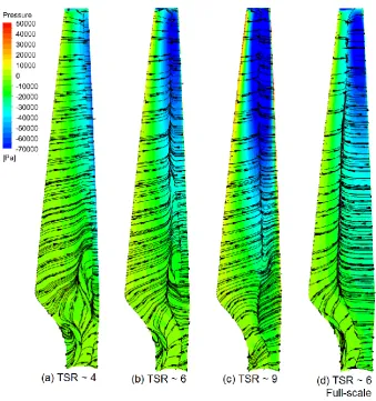
Fig. 2.11. Pressure distribution and limiting streamlines over the suction side of the blade ... 29

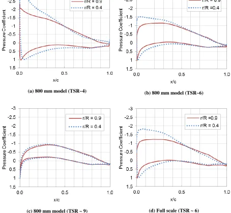
Fig. 2.12. Unsteady flow around the blade using Q-criterion of 0.004 for transient MRF simulation . 30 Fig. 2.13. Pressure coefficient over the blade surface at two radial cross sections for an inflow speed of 2 m/s at different TSRs ... 31

Fig. 2.14. Pressure coefficient at r/R = 0.7 for different TSRs of the scale model and full-scale turbine ... 32

Fig. 2.15. Comparison of CPcurves from CFD simulations with different boundary layer models ... 34

Fig. 2.16. Comparison between the CP curves of the steady and transient simulations with MRF and sliding mesh method ... 35

Fig. 2.17. Comparing the flow velocity profile around the turbine between the sliding mesh and MRF methods. ... 36

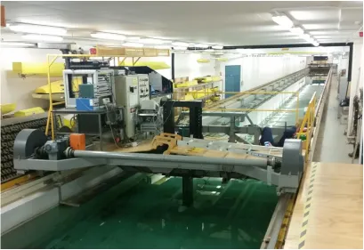
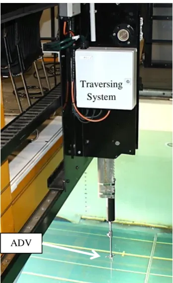
Fig. 3.1. Test setup configuration in CWC ... 41

Fig. 3.2. Schematic configuration of CWC ... 41

Fig. 3.3. Test setup configuration in Towing Tank ... 42

(14)

xiv

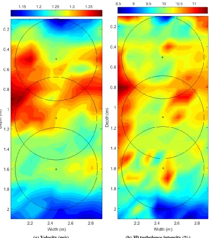
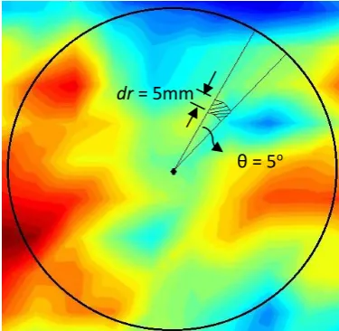
Fig. 3.5. Internal equipment of the test rig ... 43 Fig. 3.6. ADV velocity measurement ... 45 Fig. 3.7. Results from ADV measurement for a streamwise flow velocity of 1.3 m/s ... 46 Fig. 3.8. Dividing the rotor swept area to small elements for calculating equivalent inflow velocity

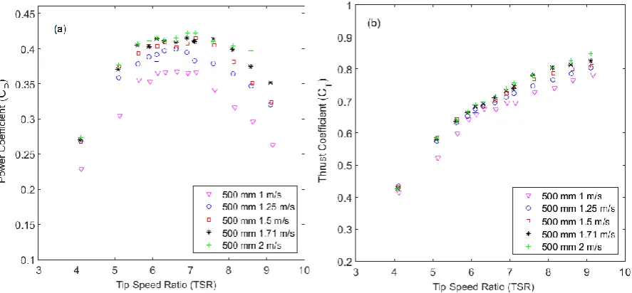
based on kinetic energy flux through the rotor swept area... 52 Fig. 3.9. Towing tank performance curves of the 500 mm diameter turbine after blockage correction53 Fig. 3.10. Towing tank performance curves of the 800 mm diameter turbine after blockage correction

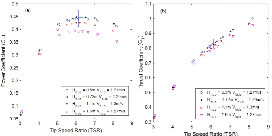
... 53 Fig. 3.11. Circulating water channel (CWC) performance curves of 800mm turbine using velocity at

the hub (a) Power coefficient (b) Thrust coefficient ... 55 Fig. 3.12. Circulating water channel (CWC) performance curves of 800mm turbine using equivalent

velocity (a) Power coefficient (b) Thrust coefficient ... 55 Fig. 3.13. Circulating water channel (CWC) performance curves of 500mm turbine using velocity at

the hub (a) Power coefficient (b) Thrust coefficient ... 56 Fig. 3.14. Circulating water channel (CWC) performance curves of 500mm turbine using equivalent

velocity (a) Power coefficient (b) Thrust coefficient ... 56 Fig. 3.15. Blockage effect on turbine performance evaluation (towing tank results) ... 57 Fig. 3.16. The effect of scaling/Reynolds number and facility bias on the turbine performance ... 58 Fig. 4.1. Comparing Lift coefficient of NACA63-618 estimated by the QBlade with the 2D wind

tunnel [21] ... 66 Fig. 4.2. Accounting for Reynolds number and shear inflow in of the turbine performance evaluation

using BEM predictions and QBlade ... 68 Fig. 4.3. Accounting for scale effect in the turbine performance assessment using CFD simulations . 69 Fig. 4.4. Comparing the methods employed for performance evaluation of 800 mm turbine ... 70 Fig. 5.1. The domains of the CFD model and the boundary conditions ... 78 Fig. 5.2. Validation of the single-phase and the VOF model for shear using fitted experimental curve

at 1.1 m depth ( case s from Table 5.1) ... 82 Fig. 5.3. The VOF model validation for depth case using AMC towing tank results ... 83 Fig. 5.4. Pressure coefficient over the turbine blade (a) at two immersion depths and (b) under case

w1 at depth of 0.76 m ... 83 Fig. 5.5. Free surface deformation due to the turbine rotation ... 84 Fig. 5.6. The VOF simulations results of torque over each blade and the total torque of turbine in two

submergence depths ... 84 Fig. 5.7. Phase averaged results from the simulation of the validation wave case at U = 1.25 m/s and

TSR= 6.5. Solid line relates to the phase-average parameter; dashed line represents the averaged values. Blue dotted line is phase-averaged and blue dash-dotted line is

(15)

xv

Fig. 5.10. The VOF simulation results of torque over each blade and the resultant torque of the turbine in condition with and without shear velocity profile at TSR ~ 6.5 and hub immersion depth of 0.76 m... 88 Fig. 5.11. Comparing the velocity distribution over the vertical plane in the VOF simulation with and

without velocity profile ... 89 Fig. 5.12. The VOF results of torque over each blade and the resultant torque of the turbine model

under wave case 1 condition at TSR ~ 6.5 and two hub immersion depths ... 90 Fig. 5.13. Phase averaged results from the simulation of the wave cases at U = 1.25 m/s and TSR=

6.5. Thick dashed line represents the time-averaged values ... 91 Fig. 6.1. Performance of the 800 mm turbine at TSR~6.5 obtained from different assessment methods

... 103 Fig. 6.2. Performance of the 500 mm turbine at TSR~6.5 obtained from different assessment methods

(16)

xvi

List of Tables

Table 1.1. Blade Geometry ... 6

Table 2.1: CFD setup ... 18

Table 2.2: Simulation time and momentum residual in steady state solutions at TSR ~ 6 ... 20

Table 2.3: Simulation time and momentum residual in transient solutions at TSR ~ 6 ... 20

Table 2.4: Sample Calculation of Grid Convergence Index for Numerical Models ... 22

Table 3.1. Details of the experimental testing facilities ... 42

Table 3.2. Uncertainty of experimental results in each facility at TSR ~ 6 (data given is +/- amount in the relevant units) ... 51

Table 5.1. Characteristics of case studies applied to the turbine in CFD simulations ... 80

Table 5.2. Cyclic fluctuations of torque over a single blade and rotor for simulation cases ... 85

Table 5.3. The turbine performance results from simulations and the AMC experiments under the wave condition ... 86

TABLE IV Blade Geometry ... 116

(17)

xvii

Nomenclature

Greek Symbols

α Local angle of attack rad

β Seabed friction -

γ Power law of velocity profile -

δ Local blade twist rad

ε Change in key variable -

P

 Precision error -

B

 Bias error -

cal

 Calibration error -

θ differential angle of the element rad

λr Local tip speed ratio rad

μ Viscosity kg / m.s

υ Kinematic viscosity m2 / s

ρ Density kg / m3

σi Root mean square of velocity fluctuations m / s

σs Standard deviation -

τ Shear stress N / m2

ϕ Key variable of simulation (Torque/Thrust) -

φ Relative flow angle rad

ψ Local solidity ratio rad

ωw Wave angular frequency rad / s

ω Rotational velocity rad / s

Ɐ Volume m3

Roman Symbols

a Axial induction factor -

a՛ Angular induction factor -

(18)

xviii

Aw Wave amplitude m

B Number of blades -

C Cross-sectional area of facility m2

CB Blockage correction factor -

CL Lift coefficient -

CD Drag coefficient -

CT Thrust coefficient -

CP Power coefficient -

dr Differential radius m

dt Time step s

dT Differential thrust N

dQ Differential torque N m

c Local blade chord m

e Relative error of key variable -

F Tip loss factor -

g Gravity m / s2

h number of mesh -

H Total water depth m

I 3D turbulence intensity -

Ix streamwise turbulence intensity -

k Wave number 1 / m

N Number of grids -

NS Number of measured samples -

pe Apparent order of mesh -

P Pressure Pa

Q Torque N m

r Local blade radius m

rf Mesh refinement factor -

R Rotor radius m

Rec Chord based Reynolds number -

S Surface m2

(19)

xix

SEE Standard error of estimate -

SSR Summed square of residuals -

SE Standard error -

t Time s

th Local blade thickness m

tn−2 t-random variable with n − 2 degrees of freedom

-T Thrust N

u Velocity vector m / s

U Freestream velocity m / s

uτ Friction velocity m/s

u՛ Velocity fluctuations m / s

u Mean velocity m / s

uw x Wave velocity in x-direction m / s

uw z Wave velocity in z-direction m / s

U1 Velocity at turbine location m / s

U2 Velocity in wake m / s

U3 Bypass velocity m / s

U Depth averaged velocity m / s

Uz Velocity at depth z m / s

Ueq Equivalent velocity m / s

Urel Relative velocity m / s

v Analogue voltage recorded by sensor Volt

Y+ Dimensionless distance from wall -

yw Distance from wall m

(20)

xx

Abbreviations

AMC Australian Maritime College

ADV Acoustic Doppler Velocimeter

ADCP Acoustic Doppler Current Profiler

AoA Angle of Attack

BEM Blade Element Momentum

BSL EARSM Baseline Explicit Algebraic Reynolds Stress Model

CAD Computer-Aided Design

CFD Computational Fluid Dynamics

CWC Circulating Water Channel

FSI Fluid-Structure Interaction

GCI Grid Convergence Index

HAMCT Horizontal Axis Marine Current Turbine

ITTC International Towing Tank Committee

KE Kinetic Energy

MRF Moving Reference Frame

MSWT MARIN Stock Wind Turbine

NACA National Advisory Committee for Aeronautics

NREL National Renewable Energy Laboratory

RANS Reynolds Averaged Navier Stokes

SPh Single-Phase

SST Shear Stress Transport

TKE Turbulence Kinetic Energy

TSR Tip Speed Ratio

TT Towing Tank

USNA United States Naval Academy

(21)

1. Chapter 1: Thesis Introduction

Chapter 1

(22)

2

1.1. Introduction

Fossils fuels are currently the main resource providing global energy requirements. Huge

dependence on this conventional source of energy is raising significant concerns. In addition

to their negative environmental impacts, given the current rate of exploitation these resources

are expected to be depleted within the next few decades. Thus, many studies are being

performed to develop various renewable energy resources as sustainable alternatives. Oceans

cover more than 70% of the earth, which store a vast renewable energy resource. The forms of

ocean energy can be categorised into tidal, wave, current, thermal gradient and salinity gradient

[1]. Tides and waves can provide predictable and consistent power generation, compared to

solar and wind energy, which are highly dependent on weather condition [2]. Global tidal and

marine current energy capacity is estimated to be in the order of 570 TWh/yr [3] well over

twice electricity consumption of Australia in 2014 [4].

Horizontal-axis marine current turbines (HAMCTs) are devices that can convert the kinetic

energy of the oceans to electricity [5]. Full scale HAMCTs are in the range of 1 MW and have

2 or 3-bladed rotors. The turbine blades rotate about a horizontal axis, parallel to the direction

of the water flow. Ocean current velocities in a range of 2 to 3 m/s are optimal for the operation

of these turbines. In those currents, a tidal turbine generates the same amount of energy as a

wind turbine four times the size. Despite the performance of a horizontal-axis turbine

depending on the current direction, they have slightly higher efficiency than vertical turbines

[6]. Some examples of HAMCTs are the AR-1000, shown in Fig. 1.1, presented by Atlantis

Resource Corporation [7], the HS1000 designed by Andritz Hydro Hammerfest [8] and the 1.2

MW SeaGen in Northern Ireland [9].

1.2. Problem Definition

In spite of recent advancements in tidal energy technology, it has not yet become technologically competitive with other renewable energy sources [10, 11]. One of the main

concerns is the reliability and performance of these devices in the harsh marine environment

[12]. Although many researchers have been striving to enhance the technology of these devices

for many years, there are not yet many commercialised HAMCTs around the world [13, 14].

To date, operational records of only a few tidal energy devices have been demonstrated [15].

Turbine performance is influenced by various parameters, such as the flow condition of

(23)

3

to ensure that the performance of a turbine is optimum for a particular site in the primary design

stages [16]. Various flow conditions that a turbine may experience, for example, are shear

velocity profile due to seabed friction, change in flow direction, turbulence and fluctuations in

the flow, depth variation and surface waves. Despite recent studies trying to assess the effect

of these conditions on the turbine performance, more investigation is required to address the

[image:23.595.161.434.205.423.2]

influence of each flow condition on the hydrodynamic characteristics of HAMCTs.

Fig. 1.1. Deployment of AR-1000 at a tidal site [7]

There are several approaches available to study the performance of a full-scale turbine,

among which selecting an appropriate and accurate method that characterises the turbine

hydrodynamics in various operational conditions is crucial. Among all of the theoretical

approaches for analysing turbine performance, Blade Element Momentum (BEM) Theory

represents the state-of-the-art. This theory is based on the assumption that each stream flow

passing through the screw disc can be analysed independently from the rest of the flow.

Therefore, the variations in the fluid dynamic quantities occur in the plane along the axial and

radial directions from strip to strip, without considering expressly the radial equilibrium among

the strips [17]. The Blade Element Momentum (BEM) theory is a useful tool to attain a quick

power prediction of a marine current turbine [18]. A comprehensive description of BEM theory

is given by Manwell, et al. [19]. Studies that have applied BEM theory to HAMCTs include

[18, 20-24].

Experimental approaches are common practice to predict the hydrodynamic characteristics

of marine systems. However, experimental tests are expensive to perform on full-scale turbines.

(24)

4

drawback of model tests is the unwanted effects of scaling that influence the viscous flow over

the turbine blades. Nevertheless, they offer a realistic condition for performance evaluation and

parametric study. Developing successful testing procedures and scaling methods has always

been a key issue to predict valid full-scale performance. Having the ability to extrapolate results

from model test data reduces some of the costs and challenges in turbine development. Besides

the scale effects, there are parameters, such as facility bias, blockage and flow conditions, that

should be taken into account when analysing the results. In this regard, different methods and

facilities are proposed to see the effects of various factors, such as facility bias, on the

performance of HAMCTs. Most facilities employed to test marine current turbines, such as

towing tanks, have no turbulence and present a uniform flow. Thus, the performance curves

developed from testing in such facilities represents the ideal case. Turbine performance in a

real environment will be different due to the flow unsteadiness, which is demanding to be

accounted for in a model test procedure. Key experimental studies on HAMCT include

[25-32].

In addition to results from the above-mentioned approaches, an accurate and detailed

performance prediction can be achieved if the assessment method considers the viscous effect

over the turbine blades. Computational fluid dynamics (CFD) is an approach that inherently

captures viscous flow. Although CFD may come with a great computation cost, the advantages

of providing a better understanding of the flow field around the blade should not be neglected

[33]. CFD is mainly being utilised as a tool for complex flow studies [34]. In addition, CFD

can be employed to improve the design of a turbine in order to optimise the performance [35].

However, due to the vast variety of methods that can be employed for performance assessment,

selecting a proper CFD approach is challenging. Some key CFD studies on HAMCT are [18,

36-42].

1.3. Research Objectives

The core aim of this work was to evaluate the performance of a horizontal axis marine

current turbine in both steady and unsteady flow conditions. To find the best practice for

performance evaluation, an in-depth investigation on the various methods and their limitations

and benefits was completed. This allows quantification of the parameters of importance relative

to the environmental conditions at a deployment site. The two overarching research questions

(25)

5

“How do flow conditions, such as shear inflow velocity, waves and submergence depth, and

evaluation parameters, such as blockage and model scale, influence the performance of HAMCTs?”

“What are the best approaches to characterise the hydrodynamic performance of

HAMCTs in steady and unsteady flow conditions?”

To address these questions, three methodologies including theory, scale model tests and

CFD modelling were employed to assess the performance of the turbine. Based on the

outcomes of this study, guiding principles are presented on how best to assess turbine

performance. Conclusions about the hydrodynamic behaviour of the turbine in different flow

conditions are also presented.

1.4. Description of Model Geometry

The experiments for this study consisted of tests on scale models in both the Towing Tank

(TT) and Circulating Water Channel (CWC) of the Australian Maritime College (AMC), University of Tasmania. The physical turbine models were two-bladed rotors, which are 1/20th

and 1/32th scale of the commercial-scale design of a HAMCT developed at the U.S. National

Renewable Energy Laboratory (NREL). The rotors and hubs , made from 6061 T6 Aluminium

alloy, were based on those designed at the United States Naval Academy [21], which have a

NACA 63-618 model blade profile. Lift and drag coefficient data for this blade is available

from Miley et al. [43] and X-Foil predictions [44]. The diameters of the two models were 500

mm and 800 mm. The lift and drag coefficients of the blades in the operating range should be

Reynolds number independent to allow scaling of the model-scale results to full-scale. The

Reynolds number independency of the lift and drag coefficient data at the operating Reynolds

number was investigated by Walker et al [21]. The blade details are provided in Table 1.1;

where r is local radius, c and th are local chord and local thickness of the blade, respectively and R is the overall blade radius. The rotors are shown in Fig. 1.2.

(26)

6

Table 1.1. Blade Geometry

Section r/R c/R th/c (%)

Twist

(deg) Shape

1 2 3 4 5 6 7 8 9 10 11 12 13 14 15 16 17 18 19 20 21 22 23 24 25 0 0.115 0.175 0.205 0.243 0.261 0.299 0.336 0.355 0.385 0.445 0.475 0.505 0.565 0.595 0.625 0.685 0.715 0.745 0.805 0.835 0.895 0.925 0.985 1 0 0.08 0.117 0.136 0.161 0.17 0.165 0.16 0.158 0.153 0.145 0.141 0.137 0.128 0.124 0.119 0.11 0.106 0.101 0.092 0.087 0.078 0.073 0.063 0.06 100 100 62.9 46 29.8 25.4 21 18.5 18 18 18 18 18 18 18 18 18 18 18 18 18 18 18 18 18 12.9 12.9 12.9 12.9 12.9 12.9 11.5 10.2 9.5 8.7 7.4 6.9 6.5 5.7 5.4 5.1 4.5 4.3 4.0 3.6 3.4 2.9 2.7 2.2 2.1 circle circle ellipse ellipse ellipse thick foil thick foil thick foil foil foil foil foil foil foil foil foil foil foil foil foil foil foil foil foil foil

The experimental results provide a solid dataset, describing the hydrodynamic behaviour of

the HAMCT. In addition, a key objective of this work was to validate the theoretical and

numerical models. The experimental dataset together with data available in the literature were

utilised for validation in this thesis. The CAD design of the turbine generated in Rhino modeller

is shown in Fig. 1.3. The CAD model was identical to the physical scale turbine, which allows

for validation of the CFD models.

(27)

7

1.5. Novel Aspects

The contributions of this study are through the application of different methodologies in

assessing the turbine hydrodynamic characteristics in conditions rarely studied. The novel

aspects of this study are as follows:

Experimental investigation of scale effect by conducting tests on two physical model sizes of the turbine. Some previous works have studied the effect of scaling on wind turbines using numerical methods. Make and Vaz [45], Giahi and Dehkordi [46], in similar efforts, conducted

some CFD simulations on the performance of wind turbines at model and full-scale Reynolds

numbers conditions. There is a lack for experimental study of scale effect in the literature. This

thesis is pioneering in evaluating the scale effect on marine turbines performance using

experimental methods.

Evaluation of the facility bias effects on the turbine performance assessment by comparing towing tank and circulating water channel results. Despite recent research by Gaurier, et al. [30] which performed experiments on a tidal turbine model in two towing tanks and two

circulating water tanks, a detailed study was needed on the parameters associated with facility

bias, such as flow condition and blockage ratio.

Quantifying the effect of shear flow velocity on the turbine performance using experiments in the CWC and CFD simulations. Although there are some previous studies on the effect of shear velocity on wind turbines, such as Bardal, et al. [47] and Wagner, et al. [48], few studies

have been performed on marine turbines, such as a numerical study by Tatum, et al. [41]. In a

recent experimental effort, Forbush, et al. [49] developed a method to account for spatial and

temporal velocity variations in performance assessment of a full-scale cross-flow hydrokinetic

turbine in an intended river. However, providing a general approach to consider shear in the

performance assessment of marine turbines was required.

A theoretical approach was employed to check the effect of Reynolds number and shear on the turbine by developing a BEM code and modelling the turbine in QBlade. Previous BEM studies on marine turbines were performed in steady condition of flow, such as [20]. In an

effort by Koh and Ng [20], the effect of Reynolds number in BEM theory accuracy was

investigated using lift and drag coefficients obtained from XFoil. This was performed using

various blade pitch angles in one uniform flow velocity. In a work performed by Masters, et al.

(28)

8

turbine using BEM. However, this thesis has employed various inflow velocities to see the

effect of Reynolds number on BEM results in addition to the influence of sheared flow in BEM

calculations.

The interaction of shear and waves on the hydrodynamic characteristics of the turbine was simulated using numerical modelling. There are some studies on wave effects on marine current turbines ([42, 51-53]) and recently an investigation was conducted by Tatum, et al. [41]

on the turbine performance under the interaction of shear and waves using CFD modelling. A

point of difference in this thesis is that two CFD models were evaluated to find the best

approach to account for shear, surface proximity and wave. The model was validated against

experimental results and then the impact of various waveforms and shear flow profiles were

studied using the validated model. Finally, the interactive effect of submergence depth, shear

and wave was investigated on the HAMCT performance.

A comparison presented, in this work, among the theoretical, numerical and experimental methods employed for the performance assessment of the HAMCT. The impacts of different parameters associated with an assessment approach or those involved in environmental

condition were examined and recommendations were provided on how to deal with them.

Although these methods are common practice among researchers, comparing all the methods

for a turbine is rare.

1.6. Thesis Outline

This work, completed in a chapter structure, consists of introduction, scientific chapters and

conclusion. The chapters follow the development of the methods employed for the performance

evaluation of the turbine, including numerical, experimental and theoretical approaches, to

study the effects of various operational parameters. The structure of the thesis is as follows:

Chapter 1: The introductory chapter defines the research problem, the research objectives

and explains the geometric models employed in this research. The novel aspects of the work

were presented with respect to other studies in this field.

Chapter 2: In this chapter, CFD approaches were compared and discussed to find an

optimum numerical method for marine current turbine modelling. The influences of using these

approaches on the numerical results were assessed against experimental results from the

(29)

9

using incompressible Navier Stokes equations, continuity and momentum conservation. Then

the CFD model setup, including geometry modelling, grid generation and solver setting in the

ANSYS CFX were presented. Two turbulence models of k- SST and BSL EARSM were applied on the model. Steady state and transient solutions using moving reference frame (MRF)

and sliding mesh method were compared. The effect of modelling a single blade instead of the

whole turbine was evaluated. Three approaches of boundary layer modelling over the blade,

including wall function, near wall method, and transitional gamma-theta model were studied.

A grid sensitivity and a Y+ study were implemented on the numerical models. Finally, the

proposed CFD approach should be able to predict the hydrodynamic characteristics of different

scales of the turbine.

Chapter 3: The third chapter presented the experimental approaches for the performance

assessment of the turbine. The performance was characterised by testing two physical scale

models. The experiments were implemented in the towing tank and the CWC of the AMC,

enabling an investigation on the effect of facility bias. Blockage and flow velocity profile are

the main differences between the two facilities. Moreover, the scale effect was studied by

comparing the results from the two scale models. The independency of the results from

Reynolds number was checked in order to predict the full-scale turbine performance.

Chapter 4: This chapter provides a comparison among the performance evaluation

methods. To see the effect of Reynolds number in BEM prediction, the larger turbine was

modelled in the QBlade, a BEM based software. To find the best BEM approach, the turbine

performance results from the QBlade using lift and drag coefficients from local sectional

Reynolds numbers were compared with the BEM model with a single reference Reynolds

number. The BEM model was developed to model the turbine in the shear velocity profile of

the CWC. The results from the theoretical models introduced in this chapter were compared

with the experimental and the numerical models in the previous chapters, which would signify

the advantages and limitations of each analysis method for HAMCT characterisations.

Chapter 5: In this chapter, the experiments on the 800 mm diameter scale model of the turbine in the CWC were presented for different depths and shear flow profiles. The CWC flow

characteristics were measured using an acoustic Doppler velocimeter. Then an experimentally

validated CFD model was developed to account for shear and surface waves. Results from the

towing tank [54] and the CWC were utilised to validate CFD model for wave and shear

(30)

10

practice for performance evaluation of the turbine in presence of wave and shear flow profile.

Finally, the hydrodynamic characteristics of the turbine under the influence of wave and shear

were assessed using the validated CFD model.

Chapter 6: The concluding chapter of this work provides a summary of the project by

presenting the key findings together with recommendations for future researchers in this field.

It also discusses the implication of findings and limitations of the approaches employed to

(31)

2. Chapter 2: Numerical Assessment of a Horizontal Axis Marine

Current Turbine under Steady Flow Conditions

Chapter 2 Numerical Assessment of a Horizontal

Axis Marine Current Turbine under

Steady Flow Conditions

A refereed journal paper was published based on this Chapter in the International Journal of Marine Energy. The citation for this journal paper is:

(32)

12

2.1. Introduction

Marine current turbines work on a similar basis to wind turbines. Therefore, a lot can be

learnt from wind turbine studies to develop performance prediction methods for HAMCTs.

Blade element momentum theory and the vortex element approach are two conventional

methods for the performance evaluation of wind turbines, shown to be applicable to marine

current turbines by many studies, such as Wu, et al. [55], and Baltazar and De Campos [56].

Despite helpful results from these two methods, an accurate performance prediction needs to

consider the viscous effect on the turbine blades. Computational fluid dynamics (CFD) is an

approach that can capture viscous flow. Although CFD may come with a great computation

cost, the advantages of providing a better understanding of the flow field around the blade

should not be neglected [33]. Thus, CFD is being utilised as a tool for complex flow studies

[34]. In addition, CFD can also be employed to improve the design of a turbine in order to

optimise the performance [35]. A detailed study was performed by Make and Vaz [45] to

analyse the scaling effect on the performance of two well-known National Renewable Energy

Laboratory (NREL) 5MW and MARIN Stock Wind Turbine (MSWT) wind turbines using

Reynolds Averaged Navier-Stokes (RANS) simulation. Giahi and Dehkordi [46] also did a

similar study on developing a RANS model to assess the effect of scaling on aerodynamic

behaviour of an NREL 2MW wind turbine.

In recent decades, by increasing the power of computers, CFD has been used extensively as

a viable tool to predict the hydrodynamics of marine current turbines. However, due to the vast

variety of methods that can be employed for performance assessment, selecting an appropriate

CFD approach is challenging. Xu [57] applied three methods of vortex lattice, boundary

element method and a RANS solver to predict the performance of a HAMCT. Based on the

developed RANS method, he proposed a design procedure and assessed the effect of

non-uniform flow on the performance. Bai, et al. [36] employed an immersed boundary method to

couple the simulation of a turbulent flow and the solid body of a three-bladed turbine using a

3D finite volume solver. Shi, et al. [58] used the viscous flow solver ANSYS CFX to predict

the hydrodynamic characteristics of a HAMCT focusing on the impact of flow separation on

turbine performance. A RANS model of a three-bladed HAMCT in unsteady flow was

developed in STAR-CCM by Gunawan, et al. [59] using the rotating reference method with a

(33)

13

In this chapter, CFD approaches for marine turbine modelling from the literature were

compared and discussed to find an optimum numerical model, compromising between

accuracy and computational time. The impact of using these various approaches was assessed

by comparing the numerical output with experimental results from the United States Naval

Academy (USNA) [21]. Pointwise mesh software was employed for grid generation. The

well-known solver ANSYS CFX was used to set up the simulations. Two turbulence models, k-

SST and BSL EARSM, were applied to the model. Steady state and transient solutions using a

moving reference frame (MRF) and a sliding mesh method were compared. The effect of

modelling a single blade instead of the whole turbine was evaluated. Three approaches of

boundary layer modelling over the blade, including wall function, near wall method, and

transitional gamma-theta model were studied.

2.2. Problem Description

The main objective of this study was to propose a CFD model that can predict the

performance of a two-bladed HAMCT in the fully submerged condition. It assumes that the

effects of the free surface and the seabed are negligible. Some common approaches in CFD

were utilised to generate the numerical models. The models were compared in terms of their assessment of the hydrodynamic performance of the turbine and their pros and cons were

discussed. The proposed CFD approach should be able to predict the hydrodynamic

characteristics of different scales of the turbine.

The turbine model was a 1/20th scale of a two-bladed HAMCT based on a design developed

at the US NREL. The blade profile was a NACA 63-618, with the lift and drag coefficients

data available from 2D wind tunnel tests [21] and X-Foil predictions [44]. The lift and drag

coefficients were Reynolds number independent for Rec > 5×105. Rec is based on the chord

length at 70% of the span. The diameter of the model was 800 mm. The blade geometry was

detailed in Table 1.1 of Chapter 1. The hub had a diameter of 41 mm and a total length of 123

mm. The CAD design of the turbine was generated in Rhino modeller and is shown in Fig. 1.3

of Chapter 1. The CAD model was identical to the physical scale turbine from the literature,

which allows for validation of the CFD results.

(34)

14 R TSR U   (2-1) 2 2 0.5 T T C R U   (2-2) 2 3 0.5 P Q C R U    (2-3)

where Q and T are torque (N.m) and thrust (N), respectively and ρ is the water density (kg/m3). 2.3. Governing Equations

To model the hydrodynamics of the turbine, the Reynolds-averaged Navier-Stokes (RANS)

method was applied to solve the incompressible Navier-Stokes equations, continuity and

momentum conservation, written in finite volume format as follows:

0

i i V S

d

dV u dn dt



 



 

(2-4)

( )

i i j j j ij i j j M

V S S S

d

u d u u dn Pdn u u dn S d

dt     _

 

       



(2-5)

where Ɐ and S indicate integration regions of volume and surface respectively; and dn is the outward normal surface vector. u is velocity vector and indices i or j = 1, 2, 3 define the direction. p is pressure and SM is a source term. If µ is dynamic viscosity, shear stress (



ij), is defined by: j i ij j i u u x x  _  _     (2-6)

The Reynolds stress term isu ui j , determined by turbulence models. k- SST (shear stress

transport) and BSL EARSM were the two models utilised in this study to predict the turbulent

flow around the turbine blades.

The k- SST model is based on the k- model in the near wall region but utilised k-

formulation in the far field. It considers the transport of the turbulence shear stress in

(35)

15

pressure gradient [60]. Because of these improvements it is commonly used in modelling of

wind and marine turbines [33].

Baseline k- or BSL is another two equation model proposed by Menter [61] to resolve the

k- model sensitivity to free stream condition. Explicit Algebraic Reynolds Stress Model (EARSM) is an extension to the BSL, which enables the turbulence model to capture the

secondary flows as well as flows with streamline curvature and system rotation [62] [63].

Therefore, BSL EARSM is expected to predict the turbulent flow around a rotating turbine

properly.

2.4. CFD Model

2.4.1. Geometry and Flow Domain

The first step in the CFD modelling was to produce an accurate geometry of the turbine and

fluid domains. The 3D CAD model, by which the physical scale turbine was fabricated, was

used for CFD simulation. Two cylindrical fluid domains were generated around the turbine to

have one stationary and one rotating domain. In addition, given the periodic condition of the

turbine geometry, the turbine together with the two domains was halved, which reduces the

number of grids and consequently the computational time of the simulations. This model is

referred to as the half turbine in this Chapter. The influence of using one blade instead of the

whole turbine in simulations was evaluated in this study. For transient solutions with the sliding

mesh method the whole turbine must be modelled. Thus, the steady state solution was used for

comparison between the half and the whole turbine.

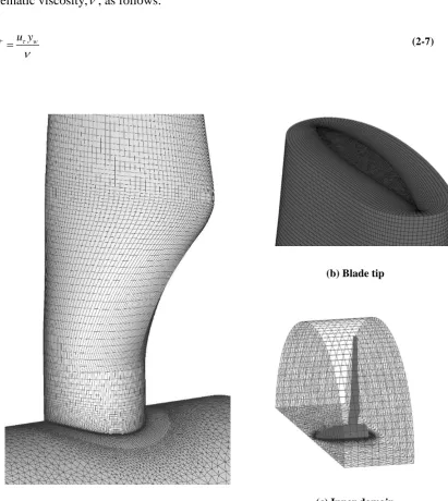
2.4.2. Grid Generation

A hybrid mesh was generated by Pointwise software, discretising the fluid domains and the

turbine surfaces. The grids over the blade surface were structured. Higher grid resolution close to the leading and trailing edges, the kink and the tip of the blade was considered to properly

discretise the curves of the blade. For the other regions including the fluid domains, the blade

tip and hub surfaces, an unstructured mesh was produced, see Fig. 2.1. The total number of

grids, including hexahedral, tetrahedral and prismatic elements, was approximately 8 million

for the whole turbine model. The number of prismatic inflation layers and the growth rate over

the blade covering the boundary layers varied depending on the required Y+. The average Y+

(36)

16

for presenting Y+ in this Chapter. Y+ is the non-dimensional wall distance which determines

the level of grid refinement. It is defined by the wall friction velocity,u_    , and fluid kinematic viscosity, , as follows:

w

u y

Y 



 _ _(2-7)

(a) Blade root and hub

(b) Blade tip

[image:36.595.87.499.129.590.2]

(c) Inner domain

Fig. 2.1. Hybrid grid generated over the turbine and flow domains for the numerical model

A Y+ in the order of 1 should be considered for the model to accurately capture the turbulent flow over the blade surfaces for the numerical models using a “viscous sub-layer modelling”

approach [33]. This method is also known as “near-wall modelling”. On the other hand, a Y+

less than 300 is recommended when a wall function applies in the turbulence model [64].

(37)

17

blades are mostly operating in the transitional flow condition. Hence, the effect of the transition

model was also checked by adding the Gamma-Theta formulation to the k- SST turbulence model. Overall, the influence of turbulence model and boundary layer model were evaluated

by using four different models as follows:

- Fully turbulent k- SST with near wall method, provided by Y+ ~ 1 - Fully turbulent k- SST with wall function, provided by Y+ ~ 30

- Transitional k- SST with near wall method, using Y+ ~ 1 and the Gamma-Theta transition model

- BSL EARSM turbulence model with wall function, provided by Y+ ~ 30

All of the above simulations were performed on a same mesh, where only the grid resolution

close to the wall has changed according to the required Y+, which had insignificant effect on

the total number of grids.

2.4.3. Solver Setup

Ansys CFX R15.0 was utilised to set up the solver. It uses a conservative element-based

finite volume method to solve the RANS model [65]. Fig. 2.2 shows the domains together with

the boundaries of the half turbine model. The condition of the boundaries, domains and

interfaces were detailed in Table 2.1. A normal velocity of 2 m/s with a turbulence intensity of

1% was set at the inlet. A zero relative pressure was considered for both the outlet and the

opening. The surfaces of the blade and the hub were specified as no slip walls. The inner

domain has a general grid interface with the outer domain. A rotational periodicity condition

was applied on the bottom faces of the two domains for half turbine model.

A moving reference frame (MRF) was described using a “frozen rotor” in ANSYS CFX to

simulate the rotation of the turbine in the steady state solution. In the MRF method, the fluid

around the blade in the inner domain was set as a MRF, while the blade and hub were stationary

relative to the inner fluid. Thus, a solution was achieved without moving the grids during the

numerical solution. The induced acceleration of the fluid was added to the momentum equation

as an extra source term. The MRF approach was performed for the transient solution as well to

(38)

18

Table 2.1: CFD setup

Boundary Condition

Inlet Outlet Opening

Blade Hub

Uniform flow of 2 m/s normal to inlet Relative Pressure = 0 Pa Relative Pressure = 0 Pa

No Slip Wall No Slip Wall

Domain Condition

Inner Domain Outer Domain

Fluid (Rotating) Fluid (Stationary)

Interface Condition

Bottom Interfaces Domains Interfaces

Rotational Periodicity General Grid Interface (GGI)

Fig. 2.2. Boundary conditions of the domains around the half turbine model

A sliding mesh method was performed to model the rotation of the rotor for the transient

solution of the whole turbine model. The transient rotor stator condition was set for the interface

between the two domains in the ANSYS CFX. The inner domain rotated at each time step for

a certain amount based on the rotational speed set for the rotor. Thus, the boundary cells of the

(39)

19

real situation when modelling the flow in rotating cases; but unlike MRF, it is computationally

demanding [66]. The result from the steady solution was set as an initial condition for the

transient rotor stator solution to help with convergence achievement in less computational time.

ANSYS CFX uses a pressure-velocity coupled method proposed by Rhie [67] to discretise

the governing equations. The high resolution scheme was chosen for discretising the advection

term as well as for the turbulent viscosity. In the transient rotor stator solutions, the second

order backward Euler scheme was used for the transient scheme.

In addition to the model scale, the CFD model of the full-scale turbine was generated to

provide a better understanding of the scale effect as well as an estimate of the full-scale

performance.

2.4.4. Solution

Torque and thrust together with power and thrust coefficients were monitored during the

solution iterations and used as criteria for solution convergence. The judgement of solution

convergence was achievement of less than 2% deviation of torque and thrust values over at

least 200 iterations. Given the higher unsteadiness for higher TSRs, for convergence

achievement in the steady condition, a number of iterations from 1500 for TSR ~ 4 to 5000 for

TSR ~ 9 were required.

The efficiency of the CFD models used for performance evaluation of the HAMCTs was

presented in Table 2.2 and Table 2.3, for the steady and transient solutions, respectively. The

tables outline the wall clock time required to achieve simulation convergence at TSR ~ 6. All

of the simulations were done on 32 cores of a high performance computing cluster with 16 GB

RAM. Total time of 3 rotations was enough to achieve convergence for the transient

rotor-stator solution using a time step corresponding to 1 of rotation. The transient time step was

defined as:

2 360

dt 





 (2-8)

The solution time for the transient sliding mesh, in Table 2.3, was high because of the need

to have a steady MRF result as the initial condition, which leads to a longer computational

time. The transient MRF simulation was run by setting the total time to 20 s and time step to

(40)

20

All the simulations were performed in double precision in order to have infinitesimal

round-off error due to the computers precision. The number of cells for the whole turbine model was

6.1 million, which was approximately halved for the half turbine model. The effect of changing

Y+ on the number mesh was insignificant. The residual of the momentum equation in the

streamwise direction for the steady and transient solutions was presented in Table 2.2 and

Table 2.3, respectively. The lower residual represents a lower truncation error, which means

higher accuracy of the converged results.

Table 2.2: Simulation time and momentum residual in steady state solutions at TSR ~ 6

CFD model

Whole turbine Half turbine

SST-wall function (Y+_{~ 30)}

SST-near wall (Y+ _{~ 1)}

SST-transition (Y+ _{~ 1)}

BSL EARSM (Y+ _{~ 30)}

SST (Y+ _{~ 30)}

BSL EARSM (Y+ _{~ 30)}

Time

(minutes) 724 1052 883 620 380 350

Residual 8.0e-05 2.2e-04 3.0e-04 8.8e-05 8.9e-05 1.0e-04

Table 2.3: Simulation time and momentum residual in transient solutions at TSR ~ 6

CFD model

Sliding Mesh - Whole turbine MRF - SST

SST BSL-EARSM Half turbine Whole turbine

Time

(minutes) 2500 2420 1477 1500

Residual 2.0e-07 1.7e-05 8.9e-08 7.0e-07

2.4.5. Grid Sensitivity

Grid sensitivity was estimated by the grid convergence index (GCI), which is actually a

measure of the discretisation error. For this purpose, three different meshes were generated

over the half turbine model by changing the grid resolution over the blade surfaces and in the

regions closer to the turbine. A factor of grid refinement greater than 1.3 was considered for

generating the meshes. The cell numbers for these three meshes were 2.15 million (coarse),

3.01 million (medium) and 4.36 million (fine). The GCI calculation in this Chapter was

performed based on the method proposed by Slater [68]. The first step to find the GCI was to

define a representative cell size:

(41)

21

where N is the total number of cells and ΔⱯi is the volume of the ith cell. Then the grid refinement factor rf = hcoarse/hfine was calculated; e.g. rf21 = h2/h1. A key variable ϕ important to the study objectives, torque in this study, was selected for error calculation. In turn, the

apparent order pe was computed using:

32 21 21

1

ln / ( )

ln( )

e e

p q p

r  

  (2-10)

21

32

( ) ln

e e p e p rf s q p rf s      _    (2-11)

where ₂₁ ₂₁ , ₃₂  ₃ ₂ and s is the sign of ₃₂/₂₁. If the relative error of the torque is

1 2

21 1

e  





 , (2-12)

Finally, GCI is obtained for the fine mesh by

21 21 21 1.25 1 e p e GCI rf   (2-13)

Table 2.4 summarises a sample of the GCI calculation performed for the three selected

meshes. It can be seen that the fine-grid convergence index is about 2%. In addition to the GCI

calculation, the grid independency of the CFD solutions was conducted on the MRF steady

technique over the different mesh resolutions. Fig. 2.3 illustrates the grid independency of the

steady solution for torque at TSR ~ 6 by showing the torque difference relative to the torque

value of the USNA results, which means |Q-QUSNA|/QUSNA. It signifies that the results are grid

independent for a cell number higher than 4 million.

2.4.6. Y+_Study

Fig. 2.4 shows the effect of Y+_{on the torque values relative to the experimental value.}

Changing the Y+ _{was important in terms of accounting for the viscous effect near the walls.}

Both the turbulence models used in this study were embedded with an automatic wall function

in ANSYS CFX R15.0. In the case of using Y+ ~ 1, the near wall method was applied to the

turbulence model. Having a Y+  20 activated the wall function method in the turbulence model. Although the higher Y+ results in less mesh density and consequently less

(42)

22

mesh independency condition was met, comparing the simulations with different Y+ resulted

in an optimal Y+ ~ 30. Later in this Chapter, this conclusion based on the correlation with the

experiments will be discussed further.

Table 2.4: Sample Calculation of Grid Convergence Index for Numerical Models

Parameter Value

N1, N2, N3

h1, h2, h3

ϕ1, ϕ2, ϕ3

rf21, rf32

pe