Macroalgal assemblages as indicators of the
broad-scale impacts of fish farms on
temperate reef habitats
by
Elizabeth Oh, BMarSc.
(University of Tasmania)
ii
Declaration
This thesis contains no material which has been accepted for the award of any other degree or diploma in any tertiary institution, and to the best of my knowledge and belief, contains no material previously published or written by another person, except where due reference is made in the text of the thesis.
Elizabeth Oh
Bachelor of Marine Science
University of Tasmania
June 2009
This thesis is an uncorrected text as submitted for examination.
Intensive fish culture in open sea pens can deliver large amounts of nutrients to coastal ecosystems. Sheltered areas with high water quality are predominately chosen for this type of mariculture, and these systems may be adversely affected by the presence of the farms. Since macroalgal community composition has been shown to be a good indicator of environmental disturbance on reef, the present study investigated the effect of salmon farms on macroalgae in a semi-enclosed coastal waterway in southern Tasmania. Data on the macroalgal community were collected from two depths at 44 sites of varying distance from twelve active fish farm leases. This included reference sites at distances of 5 km or more. The sites were widely distributed throughout the study area, and varied in their exposure to wave action. The macroalgal community composition differed significantly between sites at 100 m from fish farms and sites at 5 km or more. Sites at 400 m varied in their response to farms, with some sites showing characteristics similar to 100 m sites. Impacts varied between swell exposed sites and sites only subjected to wind-generated waves. Chaetomorpha spp. and Ulva spp. were abundant near
fish farms at exposed sites, whereas the abundance of filamentous green algae increased at sites near fish farms in sheltered sites. The percentage cover of indicator groups such as epiphytes and
opportunistic algae in total provided the best indicators of fish farm impacts on a broad scale. The percent cover of canopy forming perennial algae did not decrease near fish farms indicating that their growth and recruitment has not been greatly affected by high levels of sedimentation from fish farms or prolonged fouling by opportunistic algal epiphytes to the present, however further study is needed to examine this in more detail.
The above analysis utilised photographic quadrats to quantify community composition. Most other broad-scale sampling methods used to measure macroalgal composition require expertise to identify species in situ. However, this reduces the capacity of monitoring programs to collect large amounts
iv
Acknowledgments
I owe a huge thank you to the people who contributed to this project over the past year. A special thank you to my supervisors: Graham Edgar, Rick Stuart-Smith, and Jamie Kirkpatrick, for your guidance and support. Thank you Jamie for all your patience, encouragement and advice. Thanks Rick for your vision, advice, enthusiasm, and for lending me the camera. Thanks Graham for your wealth of knowledge and vision, and making lots of time to talk statistics. I have learnt a great deal from you all.
Thank you to Neville Barrett, Graham Edgar and Rick Stuart-Smith at the Tasmanian Aquaculture and Fisheries Institute for supporting field work in collaboration with the rare and threatened species project and the Reef Life Survey project. A huge thank you to the stunning dive coordinators Carolina Zagal, Toni Cooper and Marlene Davey, who helped with logistics and came diving in the rain, wind or shine. Thank you also to Neville Barrett, Fiona Scott, Dane Jones, Rick Stuart-Smith, Graham Edgar, Jake Virtue, Giles Barrington, and Simon Curtis, who came out in the field. Thank you also to Dane Jones for being a great dive officer, to Bob Hodgson, guardian of the boats, and to the Jones family for providing their shack at Nubeena.
Thank you to Vanessa Lucieer from the Habitat mapping group at TAFI, and Napelle Temby from TAFI/NRM South for providing spatial data. Thank you also to the Department of Primary Industries and Water for providing spatial data, especially to the marine farming division for advice. Thank you to Iain Barnes-Keoghan from the Bureau of Meterology for advice and data on Tasmanian weather. A special thank you to Neville Barrett and Fiona Scott for your advice on and enthusiasm for seaweeds! Thank you also to Catriona Macleod, Cristine Crawford, Kerrie Swadling and Jeff Ross for your advice about fish farms and lab work.
This work was also supported by The Governor’s Environmental Scholarship. Thank you to the Honourable Peter Underwood and all the sponsors for their interest and support for this project: Local Government Association of Tasmania, Hydro Tasmania, Aurora Energy Pty. Ltd., Nyrstar Hobart, Norske Skog, SEMF Pty. Ltd., Rio Tinto Alcan, and Cadbury Schweppes.
vi
Table of Contents
Declaration ... ii
Abstract ... iii
Acknowledgments... iv
Table of Contents ... vi
List of Tables and Figures... viii
Chapter 1 Introduction ... 1
1.1 Background ... 1
1.1.1 Macroalgal environmental indicators ... 1
1.1.2 Fish farming in coastal environments ... 4
1.1.3 Monitoring macroalgae ... 9
1.2 Research aims ... 11
1.3 Thesis structure ... 12
Chapter 2 Methods... 13
2.1 Study region ... 13
2.1.1 D’Entrecasteaux region ... 14
2.1.2 Wedge Bay ... 15
2.1.3 Seasonal dynamics ... 16
2.2 Experimental design... 17
2.2.1 Site selection ... 17
2.3 Data Collection ... 21
2.3.3 Manual quadrats ... 22
2.4 Data Analyses ... 22
2.4.1 Photographic quadrats ... 22
2.4.2 Statistical Analysis ... 23
Chapter 3 Results – Comparison of sampling techniques ... 29
3.1 Relationship between sites ... 29
3.2 Algal community structure ... 31
3.3 Detecting distance effects ... 36
Chapter 4 Results - The effect of fish farms ... 37
4.1 Community composition ... 37
4.2 Nutrient Pollution Indicators... 42
Chapter 5 Discussion and conclusion ... 53
5.1 Comparison of methods ... 53
5.2 The effect of fish farms ... 55
5.2.1 The nature of salmon farm impacts ... 55
5.2.2 The influence of exposure ... 57
5.2.3 The influence of depth ... 60
5.2.4 The scale of impacts... 60
5.2.5 Further research directions ... 62
5.3 Synthesis and implications for management ... 65
viii List of Tables and Figures
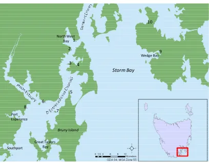
Figure 2-1 Study region. Locality of other areas mentioned in this document, 1. Tinderbox, 2. The Sheppards, 3. Roberts Point, 4. Sykes Cove, 5. Simpsons Point, 6. Ninepin Point, 7. Satellite Island, 8. Roaring Bay, 9. Parsons Bay, 10. Sloping Main ... 14
Figure 2-2 Distribution of subtidal habitats, foreshore pollution, and fish farm leases throughout the study region. . ... 19
Figure 2-3 Relationship between sites sampled, exposure, fish farm leases and the distribution of subtidal reef habitats in the study region... 20
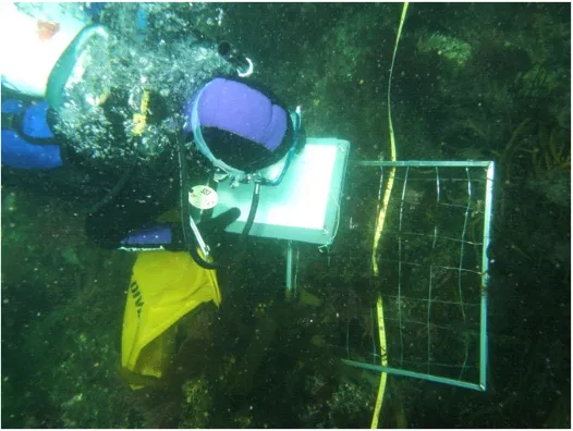
Figure 2-4 Manual quadrat sampling technique ... 22
Figure 3-1 The 2D MDS solution for the manual quadrat data. Square-root transformed data
and Bray Curtis distance measure were used. Data labels represent site numbers for each sample. ... 30
Figure 3-2 The 2D MDS solution for the photographic quadrat data. Square-root
transformed data and Bray Curtis distance measure were used. Data labels represent the site number for each sample. ... 30
Figure 3-3 Variation in percentage cover of algal layers, richness and diversity with distance using photo-quadrat methods and manual quadrat methods. . ... 33
Figure 3-4 Variation in percentage cover of algal layers, richness and diversity with exposure using photo-quadrat methods and manual quadrat methods. . ... 34
Figure 3-5 Variation in percentage cover of algal layers, richness and diversity with depth using photo-quadrat methods and manual quadrat methods. ... 35
Figure 4-1 a) PCO ordination showing exposure categories. Ordination is based on Bray Curtis similarity matrix of square root data. b) Fitted environmental vectors based on Pearsons correlation. ... 37
matrix of square root species abundance data. b) Fitted vectors of species variables correlating with CAP axis 1 (Pearsons correlation coefficient > 0.25) ... 40
Figure 4-4 Boxplots of percentage cover of indicator variables (raw data) against distance categories. ... 44
Figure 4-5 Percentage cover of opportunistic green algae throughout the sample sites on 2m depth transects. ... 49
Figure 4-6 Percentage cover of opportunistic algae in total throughout the sample sites on 2m depth transects. ... 50
Figure 4-7 Percentage cover of epiphytic algae in total throughout the sample sites on 2m
depth transects. ... 51
Figure 5-1 A reef site 100 m from a fish farm at Port Esperence ... 64
Table 3-1 Average percent cover of algal layers, total algal cover, richness and diversity measured using photographic quadrats and manual quadrats ... 31
Table 3-2 Comparison of the estimates of components of variation given by PERMANOVA analysis on manual quadrat data and photographic quadrat data. ... 36
Table 4-1 Pearson correlation values for environmental variables with the first three PCO axis ... 38
Table 4-2 Table of results, and estimates of components of variation for PERMANOVA on square-root species abundance data and Bray-Curtis distance matrix.. ... 39
Table 4-3 Pariwise comparisons for distance groups within sheltered sites and swell exposed sites. Tested using PERMANOVA using 9999 permutions. ... 39
x Table 4-6 Average abundance and occurrence of indicator species groups over the 73
transects... 42
Table 4-7 Significant environmental variables affecting the abundance of predicted macroalgal indicators. Adjusted R-squared values, F ratios and P values are shown, calculated from a fully factorial general linear model of the factors distance, depth and exposure against transformed univariate response variables. ... 45
Table 4-8 Indicator group average abundances over distance categories. Pair-wise test
groupings presented for significant terms where there was no significant interaction term between distance and exposure or depth. ... 46
Table 4-9 Indicator group average abundance and pair-wise groupings for distance and
exposure relationship.. ... 47
List of Appendices
Appendix 1 Significance tests for the difference between methods over the factors distance, depth, and exposure. Difference between the percentage estimates (MQ – PQ) was tested for the 6 algal layers, richness and diversity in each sample (N = 36). ... 79
Appendix 2 PCO ordination showing depth categories. Ordination is based on Bray Curtis similarity matrix of square root data. Fitted environmental vectors based on Pearson correlation. ... 80
Appendix 3 Average percentage cover of taxa from all samples (N = 73) against distance categories at each level of exposure. Algal layer codes are: en = encrusting, ep = epiphyte, lc = lower canopy, m = middle-storey, u = under-storey, uc = upper canopy. ... 81
Appendix 4 Box plots of percentage cover of indicator variables (raw data) against exposure categories. ... 85
Appendix 5 Box plots of percentage cover of indicator variables (raw data) against depth categories.. ... 86
on 5 m depth transects. ... 88
Appendix 8 Percentage cover of filamentous algae in total throughout the sample sites on 2 m depth transects. ... 89
Appendix 9 Percentage cover of Chaetomorpha spp. algae in total throughout the sample sites on 2 m depth transects. ... 90
Chapter 1 - Introduction
1
Chapter 1
Introduction
1.1 Background
1.1.1 Macroalgal environmental indicators
Coastal ecosystems, as the natural transition zones from land to sea, experience a high degree of pressure from anthropogenic activity. Humans have altered hydrological cycles and the flux of nutrients to coastal habitats (2002), causing system-wide impacts to estuaries, embayments, and large areas of semi-enclosed seas in many developed countries (Boesch 2002). In particular, excessive nutrients and increased rates of sedimentation have caused changes to habitat structure and diversity in temperate reef ecosystems (Worm et al. 1999; Airoldi 2003; Connell et al. 2008; Krause-Jensen et al. 2008). These changes impact on the delivery of ecosystem services to society (Costanza et al. 1997), as well as marine conservation objectives for reef areas, which are regarded as key habitats. Consequently there is a need to monitor and assess the ecological changes occurring as a result of altered water quality (Airoldi 2004).
Monitoring of nutrient levels is not solely effective in quantifying pollution pressure or impact in dynamic marine environments. The release of nutrients from a pollution source may vary diurnally, by quantity and by the nature of dispersal, creating a need for frequent sampling (Dalsgaard & Krause-Jensen 2006). Nutrient concentrations in the water column are also influenced by algal uptake (Goodsell et al. 2009). In addition, ecological impacts can rarely be predicted from nutrient concentrations, as there may be large differences among estuarine-coastal systems in their sensitivity to nutrient enrichment (Cloern 2001). Macroalgal communities on reef integrate the
effects of long term exposure to altered local environmental conditions, as they are sessile and respond to pollution over time (Munda 1993; Pinedo et al. 2007). Consequently, macroalgae are now regarded as relevant and useful indicators of environmental impact (Morand & Briand 1996; Juanes et al. 2008).
A well documented consequence of excessive nutrients in coastal reef environments is the disproportionate growth of certain types of productive, fast growing
the expense of habitat forming perennial species (Valiela et al. 1997; Worm & Sommer 2000; Gorgula & Connell 2004). These fast growing algae have been termed, ‘opportunistic’, ‘bloom forming’ or ‘nuisance’ macroalgae (Littler & Littler 1980; Valiela et al. 1997; McGlathery 2001; Krause-Jensen, 2007a).
In temperate waters, opportunistic green algae in the genera Ulva, (which now includes the genus Enteromorpha), Cladophora, and Chaetomorpha (Lavery &
McComb 1991) are the most common macroalgae reported to form blooms (Valiela et al. 1997). These algae are typically ephemeral, with a filamentous or sheet-like form, a relatively undifferentiated thallus, and a high thallus area to volume ratio (Littler & Littler 1980). Such attributes allow for fast growth and rapid reproduction when environmental conditions are ideal for growth (Littler & Littler 1980). These algae often have a high demand for nitrogen (Barr & Rees 2003), and their growth is favoured under a variety of pollution types (Guinda et al. 2008), such as sewage pollution (Soltan et al. 2001; Arevalo et al. 2007), sedimentation (Eriksson & Johansson 2005), and pollution from urbanisation (Gorgula & Connell 2004; Mangialajo et al. 2007). In eutrophic systems, dense blooms of opportunistic algae can form, and influence nutrient dynamics beyond their role as nutrient sinks (Lavery & McComb 1991), substantially altering marine community structure and function (Nelson et al. 2008).
Macroalgal blooms have been associated with the decline in coral cover in tropical waters (Fabricius et al. 2005; Littler & Littler 2007), as well as the loss of seagrass and changes in macroalgal community composition in temperate marine systems (Valiela et al. 1997; McGlathery 2001; Arevalo et al. 2007). Many opportunistic species grow as epiphytes on habitat forming algae, with epiphytic overgrowth
increasing with nutrient enrichment over large spatial scales (Russell et al. 2005). Prolonged epiphytic fouling has the potential to impair the growth of canopy-forming
Chapter 1 - Introduction
3 total macroalgal cover (due to the loss of canopy forming perennials) (Wells et al. 2007).
On South Australian temperate reefs, algal turfs (filamentous assemblages of algae <5 mm in height) have replaced canopy forming algae along urbanised coastlines,
with canopy algae declining up to 70% in cover on reefs (Connell et al. 2008). Experimental tests showed that algal turf could rapidly colonise and retain space at
high rates of sedimentation and nutrient enrichment (Gorgula & Connell 2004). A potential mechanism for the loss of canopy-forming algae is the inability for recruitment to occur amongst algal turf (Gorgula & Connell 2004), as described by Kennelly (1987) and Airoldi (2003). Additionally, recruits of the opportunistic alga
Ulva and Cladophora in the Baltic Sea have been experimentally shown to have a
high tolerance for sedimentation, whilst the perennial brown alga Fucus vesiculosus and Sphacelaria arctica did not (Eriksson & Johansson 2005). Benthic communities in the Baltic Sea change along a gradient of eutrophication, with canopy forming algae replaced by bloom forming algae towards pollution sources (Worm et al. 1999; Worm & Lotze 2006).
Recent experimental studies highlight the importance of other environmental and ecological variables that interact with the growth and dominance of opportunistic macroalgae when nutrient enrichment occurs. Opportunistic algal growth tends to decrease with increasing grazing pressure (Bokn et al. 2003; Worm & Lotze 2006), increasing canopy cover (Bokn et al. 2003; Eriksson et al. 2007), physical
disturbance (Worm et al. 2002), short water residence times (Valiela et al. 1997), or where recruitment is limited by the lack of a propagule bank (Worm et al. 1999; Worm et al. 2001). Light limitation also occurs seasonally or when over-shading by
phytoplankton blooms occur, decreasing the depth penetration of algal growth (Krause-Jensen et al. 2007b; Krause-Jensen et al. 2008).
nutrient dynamics, as they are often the subjects of conservation and do not necessarily respond in a simple manner to biogeochemical processes. It is now widely recognised that macroalgal richness, opportunistic species and cover of macroalgae provide relevant and useful indicators when monitoring environmental
disturbance on temperate reefs (Guinda et al. 2008; Juanes et al. 2008). The suitability of these indicators has been tested through the application of macroalgal
indices for environmental monitoring purposes within the European Water
Framework Directive (Wilkinson et al. 2007; Guinda et al. 2008), and observed in long-term studies of macroalgal assemblages (Shepherd et al. 2009).
1.1.2 Fish farming in coastal environments
Whilst much attention has been focussed on terrestrial derived pollution,
eutrophication from marine fish farms is also a threat to coastal aquatic ecosystems.
In 2006, aquaculture contributed 47% to the world’s fish production, and continues to grow (FAO 2009). Finfish culture in open water cages accounts for a significant part of total aquaculture production and has rapidly expanded in many coastal systems since the 1980s and 90s (HEST 2000; Sowles & Churchill 2004; Pérez et al. 2008). An increasing need exists to monitor the impacts from fish farm derived nutrient and organic matter pollution as the industry continues to expand.
Farmed finfish (excluding mullet and rabbitfish) rely on nutrient-rich compound aquafeeds as an external food source (Tacon 2004). This type of intensive fish husbandry has the potential to alter sediment and water chemistry in and around the farm area (Woodward et al. 1992). Although improved feeding technology has provided a reduction in wasted feed input, Sanderson et al. (2008) suggested that about 70% of the nitrogen and 80% of the phosphorus input to a salmon farm is released to the environment as feed wastage, fish excretion, faeces production and respiration.
Chapter 1 - Introduction
5 under and around cages has been widely documented. Negative impacts include: altered benthic infaunal species composition, increased sulphate reduction, the growth of bacterial mats of Beggiatoa spp. on the sediment surface, decreased oxygen and increased fluxes of ammonia, methane and hydrogen sulphide from
sediments (Holmer & Kristensen 1992; Black 2001; Nickell et al. 2003; Navarro et al. 2008). The presence of these conditions can have deleterious effects on fish
growth (Black, 1996); consequently the monitoring of the chemical environment is most often incorporated into fish farming practice, as is the periodic fallowing of farmed areas (Pereira et al. 2004).
Whilst the impacts of particulate waste from marine fish farms on sediments have been widely studied, impacts on the pelagic environment have not (Navarro et al. 2008). This is despite most of the nitrogen input to fish farms being lost to the environment in dissolved form, through fish excretion and remineralisation from sediments (HEST 2000). Additionally, the effect of particulate waste on sediments is often localised (< 30 m) (Ye 1991), whilst relatively broad scale and cumulative impacts may occur as a result of dissolved nutrients dispersing throughout the receiving ecosystem (Sowles & Churchill 2004).
In the pelagic environment, high ammonia and dissolved organic nitrogen levels were correlated with elevated abundances of heterotrophic microorganisms near fish farms, indicating that these microbes may be directly or indirectly affected by nutrients from fish farms (Navarro et al. 2008). Elevated abundances of
phytoplankton have also been found surrounding fish farms (Buschmann et al 2001). However this is not always the case, as many studies failed to find clear associations between phytoplankton abundance and the presence of fish farms (HEST 2000;
Alongi et al. 2003; Navarro et al. 2008; Pitta et al. 2009). This variation has been attributed to several factors. Pitta et al. (2009) recently demonstrated that
nutrients over a longer time period (Munda 1993). Growth in macroalgae may also be easier to monitor than the nutrients themselves, as concentrations of dissolved nutrients vary significantly over the day, requiring intense sampling (Dalsgaard & Krause-Jensen 2006).
The link between macroalgal growth and fish farm effluent is well established, due to the development of integrated aquaculture schemes. In these cases,
nitrogen-assimilating macroalgae reduce environmental pollution from fish farms whilst creating a profitable resource (Neori et al. 2004). The production of 92 tons of salmon can yield 385 tons (of Ulva) or 500 tons (of red algae) fresh weight of seaweed through assimilation of nutrient waste (Neori et al. 2004). Research into such polyculture systems have found that macroalgae such as Ulva (Hernández et al. 2008) effectively uptake fish farm derived nutrients, and that many macroalgal species have a preference for ammonia-nitrogen which is released from fish as metabolic waste (Sanderson et al. 2008).
From the perspective of conservation management, macroalgae of natural benthic communities near fish farms are also likely to respond to elevated nutrient levels, with potential implications for the diversity and composition of species (indicative of those already observed in eutrophic systems). Few studies have addressed this issue (Ruokolahti 1988; Ronnberg 1991; Ronnberg et al. 1992; Boyra et al. 2004; Vadas et al. 2004; Hemmi et al. 2005), although it is one of ecological and economical
significance. Ronnberg (1992), and Hemmi et al. (2005) investigated the growth of epiphytes on Fucus in the Baltic Sea, and found an increased growth and biomass of epiphytes on Fucus near fish farms, with a shift from brown and red epiphytes to green epiphytes towards fish farms. Vadas et al. (2004) found increases in the
foliose green alga Ulva near fish farms in Cobscook Bay, Maine. Boyra et al. (2004) also found significant differences between intertidal macrobenthic assemblages near
Chapter 1 - Introduction
7 Such effects could be expected to occur on a large scale, relative to most fish farm impacts on benthic communities which result from enriched particulate matter, and occur at the scale of tens of metres (Ye 1991). Due to advection, the effects of impaired water quality are likely to be detectable beyond fish farm lease boundaries
(HEST 2000). Given this, the possibility of broad scale effects of open cage fish culture on benthic macrophytic communities should be considered as a part of
ecosystem based aquaculture management. The issue is of particular relevance where numerous fish farms exist in close proximity, and where the fish farm industry is likely to expand.
This study investigates the scale and nature of fish farm impacts on temperate macroalgal communities in south-eastern Tasmania, where salmon farming has become a dominant form of aquaculture. The most concentrated area of salmon farming in Tasmanian is in the semi-enclosed water body of the D’Entrecasteaux channel and the adjoining Huon Estuary, where the industry rapidly expanded throughout the late 1980s and 90s. The waters of the area are considered relatively pristine, and fish farming may be considered a major source of anthropogenic nutrient input into the area (Macleod & Helidoniotis 2005).
Farmed salmon are carnivores, and are solely reliant on an external source of fish feed, which contains a high amount of protein. The Huon Estuary Study Team (2000) estimated that of the nitrogen contained in fish feed, 36% is retained as harvested fish, and the remaining 64% released into the estuary through metabolic waste or uneaten feed. Of this 13% is particulate and 87% is dissolved nitrogen (HEST 2000).
Biogeochemical models created for the Huon Estuary predicted that the impact of
fish farm derived nutrients would vary seasonally. In winter, dissolved inorganic nitrogen (DIN) levels are already high (due to the presence of nutrient rich marine
waters), flushing rates are high and biological uptake is low due to low light availability and low temperatures (HEST 2000). By contrast, in summer
for phytoplankton biomass). Simulations showed that doubling the 1997 fish farm loads would raise dissolved inorganic nitrogen (nitrate, nitrite and ammonia) levels by 50%, and carry risk of increased phytoplankton blooms (HEST 2000).
Consequently, the industry voluntarily put a moratorium on the amount of feed used
in the Huon Estuary (Crawford 2003), however significant growth of the industry has continued in the adjacent D’Entrecasteaux Channel. Between 1996/97 and 2006/07
Tasmanian salmon production levels have tripled from 7,647 to 23,637 tonnes
(ABARE 2008), with most of the growth occurring in the D’Entrecasteaux Channel.
The Tasmanian salmon aquaculture industry recognises that economic sustainability requires environmental sustainability, which in turn requires an understanding of the impacts of fish farms (McLeod et al. 2004). Collaborative studies between industry and scientists have investigated; (i) the impacts of organic enrichment to the
sediments near fish farms, (ii) appropriate monitoring techniques to detect these impacts, and (iii) the positive effects of fallowing practices (McLeod et al. 2004). A benthic monitoring program has incorporated this research to monitor for
unacceptable impacts of organic enrichment to the seafloor extending to 35 m from aquaculture leases. The CSIRO have undertaken biogeochemical modelling of the whole D’Entrecasteaux Channel system, including fish farm inputs. These models are extrapolated to predict the occurrence of phytoplankton blooms and conditions leading to eutrophication of the system.
The effects of fish farms on water column nutrients and dissolved oxygen are likely to extend hundreds of metres from farm sites (HEST 2000), and may impact upon macroalgal community composition in reef habitats. Such effects would be considered relatively broad-scale in comparison to other benthic impacts of fish
farms. Given the recent growth of fish farming in the D’Entrecasteaux region, knowledge is needed on the full extent and nature of impacts from fish farms so that
cumulative and regional effects can be considered as a part of aquaculture
Chapter 1 - Introduction
9 Impacts to reef habitats from fish farms in the D’Entrecasteaux Channel have not yet been researched, neither has the potential use of macroalgae as a monitoring tool been investigated. Despite this, significant reef habitats are located along the coast of this region, with two areas designated as “no-take” marine reserves (Tinderbox
and Ninepin Point). These reserves are managed for biodiversity conservation, recreation, and scientific research, three aims that could be compromised by
eutrophication associated with excessive regional nutrient input. This thesis seeks to contribute to the understanding of broad scale biological responses to fish farming in the D’Entrecasteaux Channel. Such knowledge is relevant to ecosystem based management in the study area and other locations with intensive fish farming operations. Outcomes are also relevant to the long term conservation of reef biodiversity.
1.1.3 Monitoring macroalgae
Ecological data is inherently variable, and large sample sizes are generally needed to provide the statistical power needed to describe significant patterns. An obvious issue with intensive monitoring programs is the cost and expertise required for data collection. Upon designing a sampling regime, there is often a trade off between the resolution of the data and the sample size obtained. Ultimately the choice of a sampling method strongly depends on the specific question to be answered (Dumas et al. 2009).
of SCUBA safety requirements, the physical pressures of SCUBA diving, and the costs of field data collection.
Digital sampling methods can be advantageous through speeding up data collection
in situ and eliminating the need for species identification in situ. They also provide
permanent sample records which may be re-sampled at a later date, directly compared as part of a future time series (Teixidó et al. 2009), or used as a form of
visual communication about the underwater characteristics of a sample/site (a picture speaks a thousand words). Additionally, the image analysis process is not under significant time pressure and additional information resources may be utilised. One drawback of this technique is that the image quality can be affected by environmental conditions such as water clarity, swell, and light intensity. Species may also be obstructed in a photo by shadows, canopy layer algae, or light reflection.
Nevertheless, photographic and video methods have been increasingly utilised as a consequence of improved technologies that have allowed the collection of high resolution digital images (Alvaro et al. 2008). Regardless, few previous studies have investigated the use of photographic techniques for sampling macroalgal communities. Some recent studies have demonstrated that photographic sampling can provide enough resolution to identify inter-tidal algal species (Ducrotoy & Simpson 2001), sub-tidal biotypes (Alvaro et al. 2008), and species groups of tropical benthic biota (Dumas et al. 2009), all of which are potentially useful
indicators for environmental monitoring. These studies have advocated the possible application of digital sampling techniques for monitoring benthic communities where expertise can be used for the analysis of samples, but is not necessarily available for field data collection.
This study utilises the application of photographic monitoring techniques to assess the impacts of fish farms on subtidal temperate macroalgal community composition.
A comparison of this method with manual sampling techniques is also conducted, in order to compare the application and data resolution of these two different
Chapter 1 - Introduction
11
1.2 Research aims
The rationale behind this project is to provide insight into broad scale ecological impacts of fish farming, whilst investigating the application of a digital monitoring technique that may prove useful in a general management context for monitoring macroalgal assemblages.
Primary aims of this project are:
∗ to reduce current knowledge gaps concerning the nature and extent of salmonid fish farm impacts on reef systems,
∗ to identify responses of macroalgal communities on Tasmanian temperate reefs to altered water quality, and
1.3 Thesis structure
Chapter 2 provides further details of the environmental context and seasonal
dynamics of the study area. It also outlines the design of the study, the sampling protocol, the methods used, and the statistical analyses performed to answer the research questions previously outlined.
Chapter 3 compares photographic and manual sampling methodologies.
Chapter 4 reports the results of the research on the impact of fish farms on
macroalgal community composition. Details are given for the nature, significance and distribution of the observations made throughout the study region.
Chapter 2 – Methods
13
Chapter 2
Methods
2.1 Study region
This study is focussed within the D’Entrecasteaux channel and Port Esperance, in south-eastern Tasmania (Figure 2-1). Since the mid 1980’s this region has been the main scene for the development of marine fish farming practices in Tasmania. Sites are also included on the western side of the Tasman Peninsula, near fish farms located in Wedge Bay. The D’Entrecasteaux Channel, Port Esperance, and Wedge Bay, are all part of the Bruny Bioregion, identified as part of the Interim Marine and
Coastal Regionalisation of Australia (IMCRA) scheme (Edgar et al. 1997).
General descriptions of hydrology, ecology and biogeochemical dynamics in these areas have been presented in several research publications and management reports, including those compiled for aquaculture management. The Huon Estuary Study (HEST 2000) was designed to improve understanding of chemical, physical, and biological dynamics of the estuary with particular emphasis on the potential impact of salmon farming. Jordan et al. (2002) provided an overview of hydrodynamics, nutrients and habitats in North West Bay, whilst Clementson et al. (1989)
investigated the temporal dynamics of chemical and biological parameters in Storm
Bay. An overall description and mapping of inshore habitats throughout the south-east region of Tasmania was presented by Barrett et al. (2001), for the purpose of Marine Protected Area (MPA) planning. A description of subtidal benthic macroalgae in the D’Entrecasteaux Channel was also provided by Sanderson (Sanderson 1984), and a description of seasonal variations in south-east Tasmanian phytal animal communities was provided in Edgar (1983a). The State of the D’Entrecasteaux Channel report (Phillips 1999) also provided an overview of the waterway and its catchments, their uses, values and threats.
The study area is part of Tasmania’s southern Natural Resource Management (NRM) region, which is managed by both local and state government. NRM planning
(2008). The index of ‘foreshore pollution pressure’ provides information about the distribution of stormwater, sewage, heavy industry, intensive agriculture, marina, and rural or aquaculture runoff along the coastline (Migus 2008).
Storm Bay
Wedge Bay North West
Bay
Port Esperance
Southport
.3
.7 8.
1.
6.
.5
.9
Bruny Island
Great Taylors Bay
.10
[image:25.595.130.538.150.468.2].4 2.
Figure 2-1 Study region. Locality of other areas mentioned in this document, 1. Tinderbox, 2. The
Sheppards, 3. Roberts Point, 4. Sykes Cove, 5. Simpsons Point, 6. Ninepin Point, 7. Satellite Island, 8. Roaring Bay, 9. Parsons Bay, 10. Sloping Main
2.1.1 D’Entrecasteaux region
The D’Entrecasteaux Channel is the narrow body of water between Bruny Island and the mainland of south eastern Tasmania, extending around 50 km from the north, to the south, (Figure 2-1). It is a multi-use area popular for boating, sailing, and
Chapter 2 – Methods
15 The channel receives water from Storm Bay in the north, the Southern Ocean in the south, and freshwater from the Huon and North West Bay rivers. Flushing rates are variable throughout the channel, and the maximum tidal range is 1 metre (DPIWE, 2002). The depth generally exceeds 10 m and reaches 53 m in some places (Phillips 1999). The northern end of the channel adjoins the Derwent Estuary between Pierson Point and Dennes Point, and the coast near Tinderbox is subject to some swell action, receiving water from the adjacent Storm Bay. The middle region of the
channel is largely sheltered, protected from oceanic swell by Bruny Island. Here, winds may be a major influence on the movement of surface waters. In addition, current speeds increase where water flows though narrow parts of the channel with shallow depths. The southern third of the channel is influenced by swell from the adjoining Southern Ocean, and is also influenced by the inflow of tannin stained freshwater from the Huon River. Distinctive macroalgal communities that exist at the mouth of the Huon Estuary, are adapted to low light conditions created by the overlying tannin stained waters.
Rocky shores along the coastline are primarily of sedimentary or dolerite origin. In the middle region of the channel, reefs associated with the shoreline, are low profile, rarely extending beyond 5 m depth (Barrett et al. 2001). Deeper reefs occur in areas with higher levels of exposure or current flow. Macroalgal communities found on the reef consist of temperate species. The degree of water movement over the reef influences the dominant algal species present, and the depth they extend to, with a general transition from Phyllospora comosa, Lessoniacorrugata and Ecklonia
radiata, to Fucoid and Sargassum species with decreasing wave exposure (Barrett et
al. 2001).
2.1.2 Wedge Bay
consist of sedimentary rocks or dolerite, and share most species of macroalgae with reefs in the D'Entrecasteaux Channel.
2.1.3 Seasonal dynamics
The Bruny bioregion experiences a cold temperate marine climate, and strong
seasonal influences owing to its position within the Subtropical Convergence. Water temperatures peak at 19oC in February and drop to approximately 9oC in July (Jordan et al. 2002). In winter and spring nutrient-rich subantarctic waters have a particularly large influence across southern Tasmania (Harris et al. 1987). The influence of these waters decreases over the summer period, as the oligotrophic waters of the East Australian Current (EAC) extend southwards. The strength of the EAC is subject to substantial inter-annual variability, but summer conditions within the study region are nevertheless comparatively warmer, stratified and nutrient poor than winter conditions. Nitrate levels in North West Bay and the upper D’Entrecasteaux Channel (Jordan et al. 2002), Storm Bay (Clementson et al. 1989), and at the mouth of the
Huon Estuary (HEST 2000) have been observed to show patterns indicative of these oceanographic processes, where nitrogen concentrations are high in winter and
decrease throughout spring and summer.
Chapter 2 – Methods
17
2.2 Experimental design
2.2.1 Site selection
Potential sites were identified in ArcGIS 9.3 (ESRI) by overlaying the following factors on a digital coastline map for the Bruny Bioregion:
∗ marine farming leases currently licensed for finfish farming (supplied by DPIW)
∗ benthic marine habitats of the region displaying coastal subtidal reef (supplied by the habitat mapping section of Tasmanian Aquaculture and Fisheries Institute)
∗ foreshore pollution pressure (supplied by NRM South)
∗ an index of exposure calculated for possible samples sites
Data were analysed using the Mercator projection, Geocentric Datum of Australia 1994, and Map Grid of Australia zone 55.
In order to investigate the impacts of fish farming, sample sites were selected at different distances from fish farming lease areas. In ArcGIS, buffer zones were created around active fish farm lease areas at distances of; 100 m, 400 m, 2 km and 5 km (Figure 2-2). These distances were chosen because the effects of fish farms are likely to decrease along an exponential gradient with distance from fish farms. Possible sample sites for the 100 m, 400 m, and 2 km distance categories were identified throughout the channel where these distances intersected with subtidal reef habitat, and where the area did not have significant levels of foreshore pollution pressure from sources other than fish farms. Reference sites were positioned on coastal reef areas, without significant foreshore pollution pressure, at distances from fish farms of 5 kilometres or more.
channel) and Hobart Airport (for sites on the Tasman Peninsula). It consisted of averages of wind speed and direction over the period January 1995 to December 2007. Wind energy (WE) was calculated as the square of the average wind speed (in knots) for each sector multiplied by the proportion of time the wind blew in that sector (Burrows et al. 2008). The exposure index value for numerous possible sites was then calculated as the average of WE multiplied by F at each site, plus the addition of a constant for sites directly or indirectly exposed to open ocean swell, as
in Barrett et al. (2001). For sites indirectly exposed to swell, this constant was set at the maximum exposure value for coasts affected only by local wind waves. For sites directly exposed to swell this constant was set at 1.5 times the maximum exposure value for coasts affected only by local wind waves. The distinction between swell exposed sites and sheltered (non swell exposed) sites was identified from exposure maps generated by Barrett et al. (2001), and provided a 2 level categorical version of the exposure index to be used for statistical tests.
In order to determine the effect of fish farming at different levels of exposure, sites ranging in wave exposure were included in each of the four distance categories (Figure 2-3). Sites were also spread throughout the study region as much as possible, in order to encompass the effect of fish farming over a regional scale (Figure 2-3). Selection of sample sites occurred through a process of elimination, with the aim to maximise these two variables (exposure range and spatial coverage) within each distance class. The selection of 100 m sites was limited by the availability of fish farms leases near a shoreline with reef. Choice of 5000 m reference sites was limited because of the density of fish farms within the D’Entrecasteaux area. Two reference sites were chosen at Southport, having similar aspect to those near fish farms in Port Esperance. Similarly, a reference site north of Sloping Main had similar exposure conditions to those in Wedge Bay. Ten priority sample sites were identified for each distance class, with alternative back-up sites also identified in case these were
Figure 2-2 Distribution of
subtidal habitats,
foreshore pollution, and
fish farm leases
throughout the study
region. Buffers around
Figure 2-3 Relationship
between sites sampled,
exposure, fish farm
leases and the
distribution of subtidal
reef habitats in the
Chapter 2 – Methods
21
2.3 Data Collection
2.3.1 Species Identification
Macroalgae were identified in the water to the highest possible taxonomic resolution. In cases where macroalgae could not be identified to species in situ, they were
grouped at generic level or into a functional group. For example filamentous algae were grouped into red, green and brown groups. Despite this coarse level of identification, the majority of filamentous green algae are likely to be Cladophora spp., the majority of filamentous browns are likely to be Hinksia spp., and the majority of reds are likely to be Polysiphonia spp. The coverage of benthic sessile invertebrates such as sponges, bryozoans, cnidarians and ascidians were also recorded.
2.3.2 Photographic quadrats
A total of 73 photo quadrat transect samples, from 44 sites, were collected throughout the D’Entrecasteaux channel and around Nubeena. GPS coordinates extracted from ArcGIS were used to locate predetermined field sites. Each site was first scoped with a depth sounder to determine the reef depth and extent. If the site was determined unsuitable due to a lack of reef, an alternative a priori identified site was sampled instead. Sampling was conducted between 17 November and 17 December, 2008.
As the effect of fish farms on macroalgal composition may vary with depth, sites
2.3.3
Manual quadrats
[image:33.595.202.465.354.552.2]To compare the use of the ‘manual-quadrat’ sampling technique with the use of ‘photo-quadrats’, manual quadrat samples were also conducted at a subset of field sites. A total of 36 manual quadrat transects were conducted from 35 sites. Manual quadrat samples were collected along one (or both) of the transect lines used for the photo quadrat samples at 5 m intervals (n=10 per transect), using a 0.25 cm2 quadrat with a grid of 7 wires crossing perpendicularly. Within each quadrat, the species occurring under 50 grid positions (one corner of the quadrat plus 49 intersection points) were recorded (Figure 2-4). Macroalgal species from all layers, encrusting to understorey to canopy, were recorded under each position. Time constraints on the dive meant that abundant species were estimated to some degree in most quadrats, i.e. if a species covered about half the quadrat, 25 points were recorded.
Figure 2-4 Manual quadrat sampling technique
2.4 Data Analyses
2.4.1 Photographic quadrats
Chapter 2 – Methods
23 100 pixels. Points where the underlying algae could not be identified to species were lumped into a higher category, such as ‘Sargassum sp.’, or ‘foliose red algae’. For the instances where the area was in shadow, too blurry or covered by transect line, ‘shadow’ was recorded.
Results for each transect were then exported to Microsoft Excel 2007. Percentage coverage (per transect) was calculated for each cover type. Adjustments were made so that obstruction by ephemeral epiphytic algae did not overly bias the coverage
estimate for the more permanent underlying algal community. Percentage data for the underlying community was calculated as:
Percentage (i) = points covered by type i * 100 / (total number of points - the points attributed to ephemeral coverage – the points in shadow)
Percentage data for ephemeral species was calculated as:
Percentage (i) = points covered by type i * 100 / (total number of points – the points in shadow)
2.4.2 Statistical Analysis
2.4.2.1 Comparing manual quadrats with photo quadrats
Data from the 36 manual quadrat (MQ) transect samples were paired with the appropriate subset of data from the photographic quadrat (PQ) transect samples. This dataset was analysed on a compositional, multivariate basis to compare the community information gathered by different methods. Bray-Curtis similarity matrices of the square root data for MQ and PQ methods were generated. The correlation between these matrices was tested in Primer 6+ using the 2STAGE function, selecting the Spearman rank correlation option. Non-metric MDS plots were also generated for MQ and PQ data sets in Primer 6+ to visualise how each method described the relationship between sites.
levels: 2 m and 5 m) and distance (4 levels: 100 m, 400 m, 2000 m, and 5000 m), in order to see whether the similarity between PQ and MQ methods varied over these factors. Results should be interpreted with caution as interaction terms could not be included, hence assumed non-significant, due to the sample size being too small to provide appropriate replication for a full model.
Algal species were then organised into groups according to their height dominance on the reef, so that the methods could be compared for each algal layer. Six layer
categories were generated:
• Upper canopy: canopy species that grow tall/erect, e.g. Macrocystis pyrifera, and Sargassum fallax (seasonally forming a tall canopy in sheltered sites) These may be captured differently in photo quadrats than canopy species which spread out over other algal layers
• Lower canopy: other canopy layers, e.g. E. radiata, P. comosa, D. potatorum
• Middle storey: includes most foliose red algae, and species such
Carpoglossum confluens,
• Under storey: prostrate growing plants such as Sonderapelta coriacea,
Homeostrichus olsenii, and Caulerpa beds
• Encrusting: encrusting algae, sponges, and cnidarians including: crustose coralline algae, encrusting Peyssonnelia spp., and the octocoral
Erythropodium hicksoni
To investigate the agreement between the sampling methods at each algal layer, the percentage cover estimate of each algal layer, was calculated for MQ and PQ data for each sample. Shannon diversity (H’) and Margalef species richness (d) variables were also calculated using the diverse function in Primer 6+. The differences
Chapter 2 – Methods
25 those without a normal distribution. Again, results should be interpreted with
caution as interaction terms could not be included, due to the sample size being too small to provide appropriate replication for a full model.
Finally, to test the use of photo-quadrats in detecting the impact of fish farming on macroalgal assemblages, the estimates of components of variation were compared from PERMANOVA analyses (see section 2.4.2.2) conducted on each multivariate data set. The components of variation estimate the importance of each term in
explaining the overall variation in dataset (Anderson et al. 2008), and thus can be used to compare the relative success of photo-quadrats in detecting the effect of each factor. The components of variation are analogous to the sums of squared fixed
effects (divided by the appropriate degrees of freedom) in a univariate AVOVA, for
fixed terms (Anderson et al. 2008). Factors included in the model were exposure, depth and distance (all fixed).
2.4.2.2 Community composition
Using the full dataset collected by photo-quadrats (N = 72), the percentage
abundance data of macroalgae and sessile invertebrates on each transect sample was square root transformed for multivariate procedures so that analysis was not overly biased towards the dominant species but still relied on variations in abundance. All multivariate tests based on resemblance matrices of the species variables used Bray-Curtis as the distance measure. Exposure was included in categorical tests by separating swell-exposed sites from non-swell exposed sites, creating a two-level factor.
Multivariate ordination procedures were conducted in Primer 6+ (Primer-E 2008) to visualise the distance between sites according to their benthic community
composition. Both non-metric multidimensional scaling (MDS), and principal coordinates analysis (PCO) ordinations were examined for 2D and 3D solutions.
alternative ordination procedure to non-metric MDS, which sets an a priori number of axes, and preserves the rank order of inter-point dissimilarities, rather than the dissimilarity values themselves. Ordination plots were explored for patterns and clusters, with the use of data labels and vector overlays. Vectors were produced in Primer using Pearson correlation of graph axes and the independent variables of distance, exposure and depth (these variables were first normalised).
To test the null hypothesis that community composition was not significantly
different between samples with different attributes, a PERMANOVA test was conducted using the PERMANOVA+ extension in Primer 6 (Primer-E 2008). PERMANOVA is a multivariate analogue of analysis of variance, which can be based on any distance matrix, and uses permutation methods to calculate significance values (Anderson 2001). In this case the model included the fixed categorical factors of depth, distance and the exposure index (swell-exposed versus non swell-exposed), and all interaction terms. Calculation of the Pseudo-F ratio and P value (α=0.05) was based on 999 permutations of the residuals under a reduced model. The components of variation attributed to each factor were displayed, which explain the relative importance of different terms in the model towards explaining the overall variation (Anderson et al. 2008, p. 54). The calculation of components of variation in PERMANOVA can give negative values to insignificant terms in the model
(Anderson et al., 2008). Terms with negative estimates of components of variation were consecutively pooled with the residuals starting with the one with the smallest MS, as suggested in Anderson et al. (2008). A restricted set of appropriate a
posteriori pair-wise tests was also conducted if the term distance or its interaction
with another term was found to be significant. First, 100 m sites were tested against 5000 m reference sites, to test for a significant difference. If this test was significant then 400 m sites were tested against 5000 m sites, and so on. This was done
separately at the two levels of depth and/or exposure if the interaction terms were
significant. This method acknowledged the use of 5000 m sites as reference sites and the order of the distance scale used (instead of assuming distance values were
Chapter 2 – Methods
27 In order to identify taxa that were correlated with the effect of distance, a constrained ordination procedure was conducted using the CAP function in PERMANOVA+ extension (Primer-E 2008). The CAP procedure involved a canonical discriminant analysis (between distance groups) on the PCO axes. The CAP axes are fitted through the multivariate data cloud to best discriminate between predefined groups. Diagnostics are conducted by permutation, using two test statistics (trace and largest root), and cross-validation of groups by the “leave one out” procedure. Species
variables were then correlated with the CAP axis using Pearsons Correlation Coefficient.
2.4.2.3 Nutrient pollution indicators
Following earlier authors (Steneck & Dethier 1994; Krause-Jensen et al. 2007b; Juanes et al. 2008), species were separated into categories representing their functional growth habits. ‘Opportunistic greens’ were green algal species that respond to elevated nutrients with rapid growth. This class included Chaetomorpha spp. (Juanes et al. 2008), Cladophora spp. (including filamentous green algae)
(Juanes et al. 2008), Enteromorpha spp. (Munda 1993), and Ulva spp (Munda 1993). ‘Opportunistic total’ were the opportunistic greens, brown filamentous algae, red filamentous algae(including Ceramium spp), and algal turf (Gorgula & Connell 2004; Juanes et al. 2008). ‘Epiphytic species’ included Chaetomorpha billardierii, filamentous algae, Colpomenia spp. and Asparagopsis armata. ‘Canopy brown’ species were identified as those perennial brown algae which form a canopy over the mid-storey, under-storey and encrusting species. Individual species which may respond negatively to pollution have not been identified a priori from other studies as these are likely to be perennial ‘competitive’ algae (Littler & Littler 1980; Krause-Jensen et al. 2007b) which vary by region.
The affect of pollution on the diversity and richness of macroalgae communities is also well cited (Munda 1993; Ducrotoy 1999; Wells et al. 2007; Guinda et al. 2008;
Juanes et al. 2008). Shannon diversity (H’) and Margalef species richness (d) variables were calculated using the diverse function in Primer 6+.
using univariate tests. Indicators were only tested individually where they had a high rate of occurrence amongst the samples (occurring >19 samples). General linear models were performed in Minitab15, using distance, depth, and exposure categories, and all interaction factors. Variables were transformed and tested for normality and heteroskedacity using the Ryan-Joiner test and model diagnostics. Tukeys pairwise tests were used to determine which classes were significantly different from each other.
Chapter 3 – Comparison of sampling techniques
29
Chapter 3
Results – Comparison of sampling
techniques
3.1 Relationship between sites
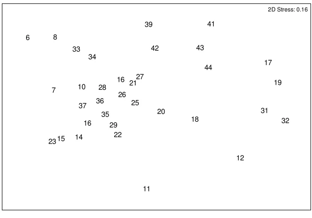
A comparison of data gained from a subset of 34 sites indicated that both manual quadrat and photographic quadrat data distinguished sites from one another in a similar pattern. There was a high correlation between MQ and PQ resemblance matrices for macroalgal community data (Spearman correlation = 0.86377). MDS ordinations of MQ data (Figure 3-1) and PQ data (Figure 3-2) show a similar
relationship between sample sites for a 2D solution. The placement of samples along
MDS axis 1 on the MQ plot was highly correlated with that on the PQ plot (Pearson correlation = – 0.955, P < 0.001). Similarly, sample coefficients on MDS axis 2 were highly correlated between the two methods (Pearson correlation = 0.701, P < 0.001).
6 7 8 10 11 12 14 15 16 16 17 18 19 20 21 22 23 25 26 27 28 29 31 32 33 34 35 36 37 39 41 42 43 44
[image:41.595.175.493.77.296.2]2D Stress: 0.15
Figure 3-1 The 2D MDS solution for the manual quadrat data. Square-root transformed data and Bray Curtis distance measure were used. Data labels represent site numbers for each
sample. 6 7 8 10 11 12 14 15 16 16 17 18 19 20 21 22 23 25 26 27 28 29 31 32 33 34 35 36 37 39 41 42 43 44
2D Stress: 0.16
Figure 3-2 The 2D MDS solution for the photographic quadrat data. Square-root transformed data and Bray Curtis distance measure were used. Data labels represent the site number for
[image:41.595.174.491.379.600.2]Chapter 3 – Comparison of sampling techniques
31
3.2 Algal community structure
The average cover of epiphytes, lower canopy and middle storey algae was very similar using MQ and PQ methods (Table 3-1). Photo-quadrats estimated a
[image:42.595.119.545.336.769.2]significantly higher cover for upper canopy than manual quadrats. The difference between methods was most pronounced for understorey and encrusting layers, where photographic quadrats detected significantly less coverage than manual quadrats (Table 3-1). MQ sampling detected significantly more total algal cover, and slightly more algal richness, and diversity. Standard error values for each variable were similar using MQ and PQ methods.
Table 3-1 Average percent cover of algal layers, total algal cover, richness and diversity measured using photographic quadrats and manual quadrats
Variable Method Average % cover Standard Error Standard Deviation T-value P-value
epiphyte MQ 39.1 5.24 30.6 -1.17 0.252
PQ 41.4 4.44 25.9
difference -2.3
upper canopy
MQ 29.0 3.90 22.7 -3.02 0.005
PQ 35.6 4.06 23.7
difference -6.6
lower canopy
MQ 7.77 1.96 11.4 -0.40 0.693
PQ 8.02 1.98 11.6
difference -0.25
mid-storey MQ 16.7 2.80 16.3 1.73 0.094
PQ 14.1 2.43 14.2
difference 2.7
under-storey
MQ 52.8 4.40 25.7 2.99 0.005
PQ 37.9 4.86 28.3
difference 14.9
encrusting MQ 21.3 4.15 24.2 4.62 0.000
PQ 3.65 1.52 8.88
difference 17.6
total algal cover
MQ 166.8 5.86 34.2 3.37 0.002
PQ 140.7 4.38 25.6
difference 26.1
richness MQ 5.22 0.24 1.39 2.46 0.017
PQ 4.75 0.32 1.86
difference 0.47
diversity MQ 2.72 0.07 0.395 4.81 0.000
PQ 2.52 0.07 0.411
Variation in algal structure, richness and diversity over distance were similar for both methods (Figure 3-3). The difference between methods over distance did not vary significantly for any of the variables, according to general linear models and Kruskal-Wallis tests (Appendix 1). However there appeared to bea tendency for photographic sampling to disproportionately overestimate upper-canopy cover when
epiphytic cover was high (100 m sites). Additionally, manual quadrats detected a slight increase in diversity and richness at reference sites (where lower-canopy cover was high), but this was not apparent using photo-quadrats. For encrusting algae, the difference between photo-quadrat data and manual quadrat data was larger at 100 m sites and reference sites. Manual sampling also detected a pattern of increased cover in under-storey algae at distances more than 100 m from fish farms, whilst photo-quadrats did not. Trends were ambiguous for middle-storey algae, which varied around 15 % cover across distance categories. Patterns detected over distance were relatively similar using both methods for epiphytes and lower canopy.
Chapter 3 – Comparison of sampling techniques 33 15 25 35 45 55 65 Epiphytes 15 25 35 45 55 Upper canopy 0 10
20 Lower canopy
5 15 25 35 Mid-storey 20 30 40 50 60 70 Under-storey 0 10 20 30
40 Encrusting algae
2.5 3.5 4.5 5.5 6.5
100 400 2000 5000
MQ PQ Richness 2.0 2.2 2.4 2.6 2.8 3.0
100 400 2000 5000
MQ PQ
Diversity
[image:44.595.113.537.180.585.2]Distance Distance
Figure 3-3 Variation in percentage cover of algal layers, richness and diversity with distance using photo-quadrat methods and manual quadrat methods. Differences between methods in trends over exposure were tested in a general linear model including exposure, depth and distance or
using Kruskal-Wallis tests for variables without a normal distribution.
10 20 30 40 50 60 Epiphyte 10 20 30 40 50 Upper canopy 4 6 8 10 12 14 Lower canopy 5 10 15 20 25 30 Mid-storey 0 10 20 30 40 50 60 70 Under-storey 0 10 20 30 40 50 Encrusting
H = 13.76 P = 0.000
3.5 4 4.5 5 5.5 6
sheltered swell exposed
MQ PQ Richness 2.2 2.4 2.6 2.8 3
sheltered swell exposed
MQ PQ
Diversity
Exposure Exposure
[image:45.595.126.534.145.653.2]F = 6.38 P = 0.017
Figure 3-4 Variation in percentage cover of algal layers, richness and diversity with exposure using photo-quadrat methods and manual quadrat methods. Differences between methods in trends over exposure were tested in a general linear model including exposure, depth and distance or
using Kruskal-Wallis tests for variables without a normal distribution.
Chapter 3 – Comparison of sampling techniques 35 20 25 30 35 40 45 50 55 Epiphyte 20 25 30 35 40 45 Upper canopy 0 5 10 15 20 25 Lower canopy 0 5 10 15 20 25 Mid-storey 25 35 45 55 65 75 Under-storey 0 10 20 30 Encrusting 3.5 4 4.5 5 5.5 6 2 5 MQ PQ Richness 2.2 2.4 2.6 2.8 3 2 5 MQ PQ Diversity
[image:46.595.121.530.144.645.2]Depth (m) Depth (m)
Figure 3-5 Variation in percentage cover of algal layers, richness and diversity with depth using photo-quadrat methods and manual quadrat methods. Differences between methods tested were
tested in a general linear model including exposure, depth and distance.
3.3 Detecting distance effects
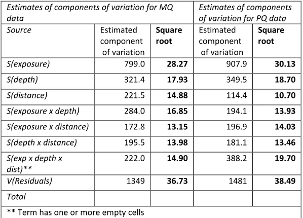
The components of variation in PERMANOVA indicated that the two methods attributed a similar amount of variation in the data to each of the model factors and
[image:47.595.184.483.455.670.2]their interaction terms (Table 3-2). The difference between the components of variation was greatest for the factor distance. Components of variation derived from the PERMANOVA on the manual quadrat data attributed 14.9 % of the variation in the data to the factor of distance. Comparatively, the photographic method picked up a weaker signal for distance (10.7 %). The difference between methods for the interaction of exposure and distance was comparatively small. Photographic methods also attributed a slightly smaller amount of variation to the exposure and depth interaction. Slightly more of the data was explained by the PERMANOVA model when manual quadrat data was used, as the component of variation for the residual term is slightly smaller.
Table 3-2 Comparison of the estimates of components of variation given by PERMANOVA using manual quadrat data and photographic quadrat data.
Estimates of components of variation for MQ data
Estimates of components of variation for PQ data
Source Estimated
component of variation
Square root
Estimated component of variation
Square root
S(exposure) 799.0 28.27 907.9 30.13
S(depth) 321.4 17.93 349.5 18.70
S(distance) 221.5 14.88 114.4 10.70
S(exposure x depth) 284.0 16.85 194.1 13.93
S(exposure x distance) 172.8 13.15 196.9 14.03
S(depth x distance) 195.5 13.98 181.1 13.46
S(exp x depth x dist)**
222.0 14.90 388.2 19.70
V(Residuals) 1349 36.73 1481 38.49
Total
Chapter 3 – Results: the effect of fish farms
37
Chapter 4
Results - The effect of fish farms
4.1 Community composition
A total of 120 taxa were identified from 73 samples in the photo-quadrat analysis. Community composition was patterned over an exposure gradient, with a clear distinction between swell-affected sites and non-swell-affected sites (Figure 4-1).
The effect of distance was independent from that of exposure (Figure 4-1 and 4-2). Both the continuous and categorical variables for exposure achieved a high
correlation with PCO axis one, which explained 31.6 % of the variance (Table 4-1). Distance had a higher correlation with PCO axis 2 which explained 11.6% of the variance in the data. The distribution of samples from each distance class along PCO axis 2 appears different at different levels of exposure, indicating an interaction effect. An interaction term between the two variables achieved a high correlation with the first two axes.
Distance Depth
Exposure Exposure category
distance*exposure
-60 -40 -20 0 20 40
[image:48.595.133.538.415.630.2]PCO1 (31.6% of total variation) -40 -20 0 20 40 60 P C O 2 (1 1 .6 % o f to ta lv a ri a tio n ) exposure category Sheltered sites Swell-exposed sites
Figure 4-1 PCO ordination showing exposure categories. Ordination is based on Bray Curtis similarity matrix of square root data. Fitted environmental vectors based on Pearson
Distance Depth
Exposure Exposure category
distance*exposure
-60 -40 -20 0 20 40
[image:49.595.130.541.83.308.2]PCO1 (31.6% of total variation) -40 -20 0 20 40 60 P C O 2 (1 1 .6 % o f to ta l va ri a ti o n ) distance 100 400 2000 5000
Figure 4-2 PCO ordination showing distance categories. Ordination is based on Bray Curtis similarity matrix of square root data. Fitted environmental vectors based on Pearson
correlation. The circle represents perfect correlation of 1.
Table 4-1 Pearson correlation values for environmental variables with the first three PCO axis
The PERMANOVA analysis (Table 4-2) revealed significant effects for the factors:
exposure (Pseudo-F=25.70, P=0.001), distance (Pseudo-F=2.41, P=0.001), depth (Pseudo-F=2.70, P=0.001), and the interaction factors: exposure by distance
(Pseudo-F=2.41, P=0.001), and exposure by depth (Pseudo-F=2.46, P=0.001). The components of variation attributed to each factor revealed that exposure explained the most variation within the data (34.8%), followed by the interaction factor exposure by distance (16.4%). Distance alone explained a further 11.6%.
Distance Depth Exposure Exposure
category
Distance* Exposure PCO AXIS1
(31.6% of total variation)
-0.0282 0.1079 -0.8708 -0.8622 -0.4262
PCO AXIS2
(11.6% of total variation)
0.2301 0.1106 0.0218 0.0301 0.3284
PCO AXIS3
(9% of total variation)
[image:49.595.124.535.425.532.2]