i
Validation of the SatGEM Velocity
Dataset using Argo Data
by
Christopher Roach
Bachelor of Science, University of Tasmania
A thesis submitted in partial fulfilment of the requirements of the Bachelor of Antarctic Studies with Honours Institute of Antarctic and Southern Ocean Studies (IASOS)
i
Declaration
I hereby declare that the thesis contains no material which has been accepted for the award of any other degree or diploma in any tertiary institution and that to the best of my knowledge and belief, the thesis contains no material previously published or written by another person except where due reference is made in the text of the thesis.
Christopher Roach
ii
The 4D SatGEM velocity model of the Southern Ocean has been derived from satellite altimetry and a Gravest Empirical Mode (GEM) model of temperature and salinity. The validity of the SatGEM model is assessed in this study by numerical forward modelling of Argo float trajectories through the 4D velocity fields.
Univariate statistical analysis of simulated and actual path lengths, together with analysis of the misfit between simulated and actual surfacing positions, suggests that the SatGEM model provides an adequate representation of the gross features of the Southern Ocean. However, on a local scale there is significant variability in misfit due to a combination of statistical fluctuations, the limited SatGEM model resolution and complex local velocity fields.
A high proportion of large relative misfit cycles are apparent for short Argo path lengths suggesting that the Argo float trajectories in these areas may be strongly influenced by complex small-scale flow features that cannot be adequately resolved in the SatGEM model. Argo float cycles with path lengths in excess of 50km and small relative misfits are effectively randomly distributed. However statistically significant clusters of large relative misfit cycles are apparent particularly in areas of known small-scale eddy current development such as east of the Kerguelen Plateau and also in the Brazil-Falklands Convergence where GEM models based on satellite altimetry are known to be inaccurate. The angular misfit for medium and small relative misfit Argo cycles is normally distributed suggesting that variability in this case arises due to statistical processes. The uniform distribution of angular misfit for large relative misfit cycles is suggestive of more random chaotic processes likely related to flow bifurcations in zones with complex velocity structure. In these cases the relative misfit is highly sensitive to the initial descent position of the float in the velocity model.
iii
I would like to acknowledge and thank the following people:
My supervisors, Professor Nathan Bindoff and Dr Helen Philips for the guidance and assistance they provided over the course of my honours project. Nathan, thanks for finding the time out of your busy schedule over the last month to help with my interpretation of results. Helen, thanks for reading all the drafts I sent you, I hope you didn’t mind my all too frequent emails clogging your in box.
Andrew Meijers for creating the SatGEM fields; providing advice on navigating the dataset and giving me access to the sea surface height fields used in SatGEM creation.
Thanks to my dad, Michael, for all the late nights spent proof reading my numerous rough drafts and many helpful suggestions during the analysis.
Dr Julia Jabour, Dr Kelvin Micheal and the other staff of the Institute for Antarctic and Southern Ocean Studies and the Antarctic Climate and Ecosystems CRC for the support provided during the coursework.
To my fellow IASOS honours students, Hamish and Nick and to all the masters’ students I shared the office with.
I would also like to acknowledge Phil Morgan, Lindsay Pender and the other CSIRO staff who developed and made publically available the SEAWATER toolkit for Matlab (http://www.cmar.csiro.au/datacentre/ext_docs/seawater.htm).
The data used in this study were collected and made freely available by the International Argo Project and the national programs that contribute to it.
iv
Abstract ii
Acknowledgements iii
1. Introduction 1
1.1 Background 1
1.2 Aims and Objectives 1
1.3 Methodology 2
2. Literature Review 4
2.1 The Southern Ocean 4
2.2 The Argo Program 8
2.3 Estimating Subsurface Structure from Surface Measurements 11 2.4 Development of the Gravest Empirical Mode Technique 13 2.5 A High Resolution GEM of the Southern Ocean 18
3. Datasets 27
3.1 The Velocity Dataset 27
3.2 Argo Data 29
4. Model Development 32
4.1 Model Development and Implementation 32
4.2 Model Components 33
4.3 Model Output 43
5. Data Preparation and Model Validation 45
5.1 Data Pre-Processing and Selection of Model Settings 45
5.2 Testing the Model 46
6. Analysis Methods 52
6.1 Output Data Processing and Definitions 52
6.2 Correlation Coefficients and R2 Values 53
6.3 Relative Misfit and Relative Path Length 53
6.4 Variance and Histograms of ε, Pargo, Psim and θ 54
6.5 SatGEM Performance, Frontal Features and SSH 54
6.6 Depth Relationships 55
6.7 Temporal Relationships 55
6.8 Comparison with Random Paths 55
7. Results 57
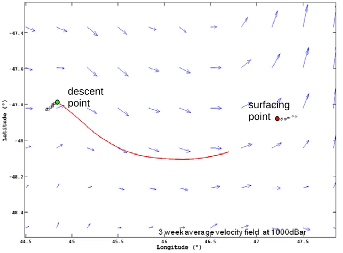
7.1 Example Trajectories 57
7.2 Geographic Distribution of Float Data 60
7.3 Path Length and Misfit 61
7.4 Histograms and Statistics 68
7.5 Correlation Coefficients and R2 Values 73
7.6 Frontal Features and SSH 77
7.7 Temporal Variability 83
7.8 Depth Relationships 85
7.9 Comparison with Random Data 86
8. Discussion and Conclusions 89
8.1 The Numerical Model 89
8.2 SatGEM Validation 89
8.3 Further Work 90
9. References 92
v
Appendix 3: descend 104
Appendix 4: parking_depth 106
Appendix 5: profile 108
Appendix 6: time_elapsed 110
Appendix 7: gen_lon_axis 111
List of Figures
Figure 2.1: Major currents and other features of the Southern Ocean.. 4
Figure 2.2: Schematic map of the principal fronts of the Southern Ocean. 5
Figure 2.3: Schematic diagram of the overturning circulation. 7
Figure 2.4: Outline of a typical Argo float cycle. 10
Figure 2.5: Real and simulated temperature and salinity sections along the
WOCE SR3 line. 16
Figure 2.6: Temperature residuals and salinity residuals in φ –longitude
space. 17
Figure 2.7: Cross section of GEM T field at 145E. 20
Figure 2.8: Fraction of variance captured by the static GEM T and S fields 21
Figure 2.9: Real and simulated temperature and salinity sections for the
WOCE P16S survey line 23
Figure 2.10: Percentage variance captured by time varying (SatGEM) T and
S fields.. 24
Figure 3.1: Flow chart showing the algorithm used in single_cycle 36
Figure 3.2: Flow chart showing details of the single_float algorithm 38
Figure 3.3: Flow chart showing the algorithm used in descend,
parking_depth and profile. 40
Figure 5.1: Test trajectories for 1 minute, 5 minute, 15 minute, 30 minute, 1
hour and 2 hour time steps. 46
Figure 5.2: Interpolated velocities vs depth for two descent phases and
expected velocities vs depth 47
Figure 5.3: Histogram of residuals between expected velocity and velocities
produced by depth interpolation. 48
Figure 5.4: Sample output from a test run of the model in a spatially
uniform time-varying field. 49
Figure 5.6: Histograms of residuals between expected velocities and
interpolated velocities. 50
Figure 5.7: One trajectory of the model (red) in a temporally static,
vertically uniform but spatially varying velocity field compared with
streamline output for the same field. 51 Figure 6.1: Schematic diagram of Argo trajectory variables. 52
Figure 7.1: Example of a simulated Argo float trajectory in a relatively
simple velocity field with corresponding small misfit in surfacing position. 57
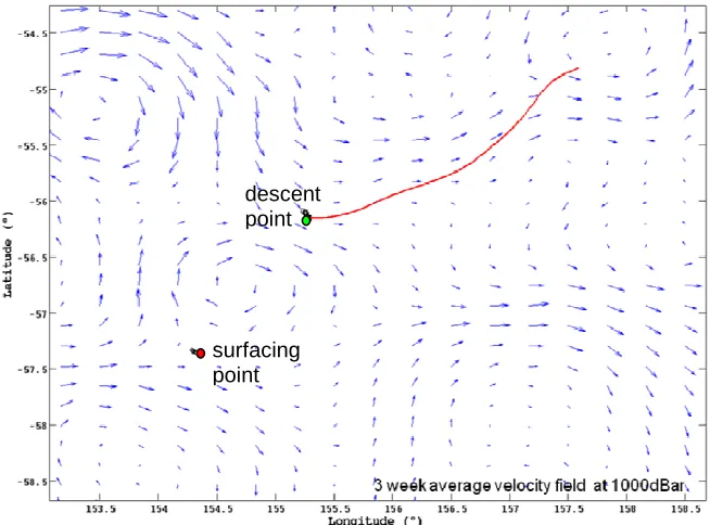
Figure 7.2: Example of a simulated Argo float trajectory in a relatively
vi
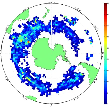
Figure 7.4: Circumpolar density of data points (by descent location) in 2° by
2° cells. 60
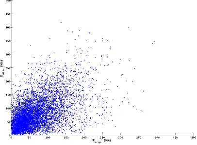
Figure 7.5: Scatter plot of |Psim| vs |PArgo|. 61 Figure 7.6: Argo path lengths (km) gridded on to a ¼° by ¼° grid. 62
Figure 7.7: Simulated path lengths (km) gridded on to a ¼° by ¼° grid. 63
Figure 7.8: Scatter plot of misfit (ε) vs |PArgo|. 64 Figure 7.9: Scatter plot of εr vs |PArgo|. 65 Figure 7.10: Circumpolar distribution of all float cycles sorted into three
categories based on εr. 66
Figure 7.11: Misfits (km) gridded on to a ¼° by ¼° grid. 67
Figure 7.12: Relative misfits gridded on to a ¼° by ¼° grid. 68
Figure 7.13: Histograms of component of Pargo and Psim 69 Figure 7.14: Histograms of latitudinal and longitudinal components of
misfits. 70
Figure 7.15: Histograms of misfit components 71
Figure 7.16: Histogram of the angle between Pargo and Psim 72 Figure 7.17: R2 between |Psim| and |PArgo| for 5x5 cells. 74 Figure 7.18: R2 for Latitudinal and Longitudinal components of Psim and
PArgo 75
Figure 7.19: Distribution of float cycles with large and small misfits 78
Figure 7.20: Ratio of float cycles with εr>1.25 and PArgo>50km to all float
cycles on a cell by cell basis for a 5° x 5° grid. 79
Figure 7.21: Scatter plots of εr vs SSH for all data (top) and Pargo>50km
(bottom). 80
Figure 7.22: Ratio of cycles with low and high εr to total number of cycles
vs SSH 81
Figure 7.23: Fraction of cycles with high and low relative misfit
components along SSH contours and across SSH contours. 82
Figure 7.24: Relative misfit as a function of date shown on a linear axis and
log axis 83
Figure 7.25: Fraction of data in 3 month bin with relative misfits of under
0.3 and over 1.25 84
Figure 7.26: Argo cycles per 3 month period, 2002-2007. 84
Figure 7.27: Scatter plots of relative misfit vs depth at descent location 85
Figure 7.28: Fraction of cycles with high and low relative misfit vs depth at
descent location 86
vii
Table 2.1: Defining Features of Southern Ocean water masses 6
Table 3.1: Data from Argo meta files used within the model 31
Table 3.2: Data from Argo traj files used within the model 31
Table 4.1: Input arguments required by single_float. 34
Table 4.2: Input arguments for the function descend. 39
Table 4.4: Input arguments for the function parking_depth. 42
Table 6.1: Peak SSH values associated with frontal features. 55
Table 7.1: Correlation coefficients and R2values for 30° longitudinal segments of the Southern Ocean and for the ACC
76
Table 7.2: Correlation Coefficients and R2 values for Psim and Pargo using the
SatGEM model and a synthetic dataset of random paths.
1
Chapter 1: Introduction
1.1 Background
Over the past two decades a number of significant advances have occurred in the field of physical oceanography. Major programs like the World Ocean Circulation
Experiment (WOCE) and the Argo program have dramatically increased the resolution of the hydrographic coverage of the world’s oceans. The coverage and quality of satellite altimetry data has improved substantially and new analysis techniques have been developed.
The Gravest Empirical Mode (GEM) method is an example of a new analysis technique which seeks “low dimensional projections of the leading order dynamics of the ocean” (Sun and Watts 2001). GEM techniques have been combined with the use of inverted echo sounders or satellite altimetry to create reconstructions of the sub-surface temperature, density and salinity structure of regions of the ocean with a high degree of accuracy (Meinen and Watts 2000; Sun and Watts 2001; Watts et al. 2001; Mitchell et al. 2004; Nardelli and Santoleri 2005). With the extension of GEM techniques from 2D to 3D datasets (Sun and Watts 2001; Meijers et al. 2009b) and improvements in resolution it has become possible to use the resulting temperature, salinity and density fields to produce density driven (geostrophic) velocity fields. These velocities by definition lie parallel to streamlines and proxies for streamlines such as contours of sea surface height (SSH).
1.2 Aims and Objectives
While GEM-derived geostrophic velocities have been used to estimate transport since Meinen and Watts (2000) first applied the GEM-techniques to the North Atlantic the creation of high resolution, temporally varying 3D velocity fields is a recent
development (Meijers et al. 2009b, 2009a). These new velocity fields for the Southern Ocean (SatGEM fields) have undergone only limited tests and validation. The
principal aim of this study is to attempt to further validate the SatGEM velocity fields by comparison with velocity information derived from Argo float data.
2
mixing may either not be well resolved or else missed entirely by the SatGEM fields. The temporal and spatial scale of the SatGEM fields also means that features with duration of less than 7 days or smaller than 1/3° cannot be resolved. Features up to twice these dimensions may be only poorly resolved.
In contrast to the SatGEM fields subsurface drifters such as Argo floats are sensitive to the contribution of all ocean current systems. As a result in regions in which flow components not resolved by the SatGEM process are significant a degree of divergence between Argo data and the SatGEM fields is to be expected. The second major aim of this project is identify and investigate major discrepancies between the two datasets as a means to identify regions where processes other than geostrophic flow may make a significant contribution to the overall velocities.
Identification of regions of non-geostrophic flow is important in understand processes such as the Meridional Overturning Circulation which is a major element of the global climate system.
A final goal of this study is to examine relationships between external variables such as sea surface height, depth and time on the performance of the SatGEM velocity model.
1.3 Methodology
3
4
Chapter 2: Literature Review
2.1 The Southern Ocean
Currents and Fronts
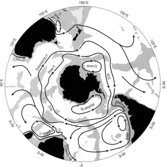
[image:12.595.160.488.295.624.2]A number of currents play a role in the dynamics of the Southern Ocean. On the northern fringes of the Southern Ocean the subtropical gyres dominate. Further south lies the Antarctic Circumpolar Current (ACC) and adjacent to the Antarctic land mass itself gyres occur in the Weddell and Ross Seas. A map of these features is shown in Figure 2.1.
Figure 2.1: Major currents and other features of the Southern Ocean.
From Rintoul et al. (2001).
5
water around the globe and forming a vital link between the ocean basins. The ACC is deep reaching and as a result its path is heavily influenced by the bottom topography.
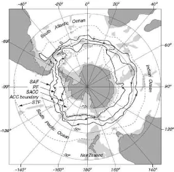
[image:13.595.169.508.325.662.2]The boundaries between the various regions of the Southern Ocean are marked by sharp transitions between water masses known as fronts (Stewart 1997). Generally, four major circumpolar or near circumpolar fronts (Figure 2.2) are recognized (Orsi et al. 1995): the Subtropical Front (STF, blocked by South America); the Subantarctic Front (SAF); the Polar Front (PF) and the Southern ACC Front (sACCf or SACC). The criteria used to define these fronts have varied considerably from study to study, for examples see Belkin and Gordon (1996). This has resulted in discrepancies in the locations of fronts (Sokolov and Rintoul 2007). In addition to the circumpolar fronts two minor fronts (the Scotia front and an unnamed front) separate the Weddell and Ross gyres from the ACC.
Figure 2.2: Schematic map of the principal fronts of the Southern Ocean.
From Stewart (1997), after Orsi et al. (1995). Shaded areas indicate depths of 3000m
6
Based on studies in the Drake Passage it was long believed that transport along the ACC was concentrated in a number of continuous and deep jets associated with the circumpolar fronts (Rintoul et al. 2001). The advent of high resolution models; remote sensing of the jets and higher resolution observations have since shown that the ACC is considerably more complex and is actually composed of (Hughes and Ash 2001): “a complex interweaving of jets, breaking and joining, beginning and ending”. A number of these jets are associated with the temperature and salinity features which older studies have used to define frontal location and are thought to account for some of the discrepancies in frontal positions in those studies. Similar studies (Sokolov and Rintoul 2007) also indicate that frontal structure is also more complex than previously believed.
The Overturning Circulation and Water Masses
While the circumpolar transport of the ACC is the dominant feature of the Southern Ocean the weaker meridional overturning circulation plays a very significant role in global climate. The circulation is dominated by six major water masses, the names and properties of which are shown in Table 2.1.
Table 2.1: Defining Features of Southern Ocean water masses.
The densest of these water masses is the cold and saline AABW which originates on the continental margins of Antarctica, most notably in the Weddell Sea. Further up the
Water Mass Temperature
(°C) Salinity (psu) Other Characteristics Sources Subantarctic Mode Water (SAMW)
4-15 34.2-35.8 (Hanawa and
Talley 2001)
Antarctic Intermediate
Water (AAIW)
3-5 (Potential
temperature)
34.2-34.4 (Gordon 2001)
Upper Circumpolar
Deep Water (UCDW)
1-2 (Potential
temperature)
34.2-34.4 Oxygen
minimum
(Gordon 2001)
(Orsi et al. 1995)
North Atlantic Deep
Water (NADW)
4 35 (Stewart 1997)
Lower Circumpolar
Deep Water (LCDW)
1-2 (Potential
temperature)
34.2-34.4 Salinity
maximum
(Gordon 2001)
(Orsi et al. 1995)
Antarctic Bottom Water
(AABW)
<-1 (Potential
temperature)
7
water column sits the LCDW, NADW and UCDW, south of the Polar Front both these water bodies extend to the surface. North of the Polar Front the AAIW and subsequently (north of the SAF) the SAMW dominate the near surface layers of the Southern Ocean.
[image:15.595.115.542.340.561.2]The overturning circulation (Figure 2.3) is largely dependent on the balance between the southwards flow of the deep waters and the northward flow of AABW and surface waters north of the PF (Rintoul et al. 2001). It has been surmised that this process is at least partially driven by Ekman (wind driven) transport: Over much of the Southern Ocean westerly winds dominate (causing northward Ekman transport), reaching a maximum in the vicinity of 50°S; further south winds are weaker and more variable. This results in divergent Ekman transport which causes upwelling of the deep waters.
Figure 2.3: Schematic diagram of the overturning circulation. From Speer et al.
(2000).
8
2.2 The Argo Program
One of the major problems for Oceanographers has been the limitations on quality, quantity, geographic and temporal coverage of data. The development of the
expendable bathythermograph (XBT) in the 1960s and the World Ocean Circulation Experiment in the 1990s (Roemmich et al. 1998) have done much to improve the extent and quality of coverage, however many limitations still remain. XBTs are principally deployed from ships of opportunity, and as such, the resulting data is mainly restricted to major shipping lanes and the measurements only provide
temperature profiles. The WOCE survey provided high quality data across the entire water column, but even given seven years of work the spatial coverage remained sparse. A solution to some of these problems has been developed in the form of the Argo program.
The Argo program is a multi-national project to deploy and maintain an array of profiling floats to give global coverage of the upper ocean (Roemmich et al. 2001). The array consists of over 3000 floats spread throughout the world’s oceans, each capable of taking temperature and salinity profiles to depths of around 2000m. The array produces over 100,000 profiles per year (Park et al. 2005). As part of the requirements of the Argo program these temperature, salinity and trajectory data are made available to the public via a number of data centres. These data are available in both near real time and delayed time, the latter with more stringent quality controls.
History
The Argo program is the latest in a long line of oceanographic experiments to make use of sub-surface floats. The use of sub-surface floats was pioneered by John Swallow in 1955 (Gould 2002) when he produced the first SOFAR (SOund Fixing And Ranging) floats. These floats consisted of a simple length of aluminium tubing with an electronic circuit and batteries sealed within the tubing and a transducer hanging below, producing a periodic acoustic signal. By triangulating the signal from multiple receivers it was possible to establish the float’s location.
9
ranges of up to 700km (Warren and Wunsch 1981). During the 1980s RAFOS (reverse SOFAR) floats were developed (Gould 2002). Like the SOFAR floats the RAFOS system relied on acoustic techniques to locate the float. However, unlike the SOFAR system RAFOS had the receivers fixed to the float and the signals transmitted from fixed stations. The float would then store the location data generated by
triangulating the sound sources until a pre-set time when it would surface and transmit the data to a satellite.
With the advent of the WOCE program during the 1990s RAFOS floats were supplemented by the introduction of Autonomous Lagrangian Circulation Explorer (ALACE) floats (Gould 2002). ALACE floats could be set to maintain a desired depth for a period of time before surfacing then descending and repeating the process. Unlike the earlier generations of floats, ALACE floats did not make use of acoustic tracking; data on the location of a given float was obtained solely from fixes obtained by satellite when the float periodically surfaced. This had the downside of losing some of the details of movements in between the surfacing times. Towards the end of WOCE a number of ALACE floats were equipped with sensors for obtaining profiles of temperature and/or salinity while surfacing; producing Profiling ALACE floats (PALACE).
10 Argo Floats
With the exception of some limited use of fixed profiling devices in the Arctic the vast majority of data collected by the Argo project is sourced from profiling floats. Currently the vast majority of deployed Argo floats are of three main models: APEX, SOLO and Provor. All of these float models have similar characteristics: a nominal life time of 4 years or between 150 and 170 cycles and a maximum operating depth of about 2000m. All Argo floats use an external hydraulically operated bladder to control depth. By adjusting the volume of the bladder the volume and hence density of the float can be changed, allowing the float to rise or sink until neutral buoyancy is achieved.
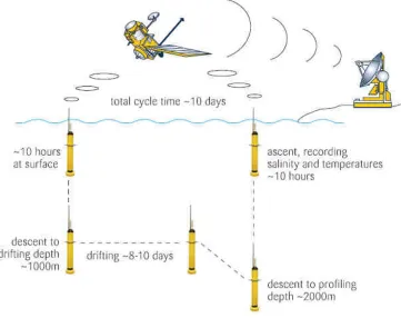
[image:18.595.138.499.326.612.2]An Argo float cycle (Figure 2.4) consists of four distinct phases. First is the surface phase during which data is transmitted to satellites.
Figure 2.4: Outline of a typical Argo float cycle. From Gould (2006).
11
greater depth. On average an Argo float cycle lasts for 9.5 days, of which 9 hours are spent on the surface (Lebedev et al. 2007).
Despite the use of the PALACE floats to estimate velocities of the deep Ocean during WOCE the use of Argo floats for a similar purpose has been limited.
2.3 Estimating Sub-Surface Structure From Surface Measurements
There are currently several major methods by which surface measurements can be used to model the sub-structure of a given region of ocean. Most older methods are based around the use of Single Empirical Orthogonal Function (sEOF) decomposition of hydrological profiles to indentify a correlation between the sEOF modes and a surface measurement (Nardelli and Santoleri 2005). More recently developed methods are based around the use of the Gravest Empirical Mode (GEM) technique, in which a ‘unique’ profile is associated with specific values of a function of the integrated density anomaly of a column of water.
The use of sEOFs to reconstruct a temperature or salinity profile from surface data originated in the late 1980s (Carnes et al. 1994). A typical method used for sEOF reconstructions was described by Pascual and Gomis (2002):
A set of profiles located at (x,y) with data recorded at a number (N) of common pressure levels is denoted by αx,y(p). By subtracting the mean historical profile from each profile in αx,y(p) a set of anomaly profiles, α’x,y(p), can be created.
From the profiles in α’x,y(p) a NxN matrix can be constructed and rearranged so as to
obtain a set of orthogonal eigenvectors (the EOFs) and the ratio of a given eigenvector to the sum of the eigenvectors will yield the fraction of variance explained by that particular EOF. Profiles can then be reconstructed from the equation:
∑
= i
i i
y x
estimated , (p) 1A(x,y)EOF(p)
α
Where A1 to Ai are the magnitudes of the corresponding EOFs.
Thus, if the amplitudes of each EOF can be associated with a surface property a profile of a given variable can be reconstructed. In practice it is usually not necessary to use all EOFs as a reduced number will usually account for the majority of the variance.
12
acoustic travel time or dynamic height. This approach allows the creation of a look up table of profiles of the variables; with each profile corresponding to a particular value of the function of density. In theory a given value of the function of density could correspond with a vast number of different temperature (T) and salinity (S) profiles. However the GEM technique works because it has been established empirically (Meinen and Watts 2000) that for some regions of the ocean each value of the density function is associated with a set of very similar profiles.
In addition to the GEM and sEOF methods two other techniques, coupled pattern reconstruction (CPR) and multivariate EOF reconstructions (mEOF), have been introduced in recent years. While initial work in the North Pacific (Nardelli and Santoleri 2005) suggests both these methods may result in greater accuracy than sEOFs and GEMs there has not been sufficient studies to establish the utility of mEOFs and CPRs more generally.
Comparison of GEM and sEOF Techniques:
There have been few direct comparisons of the ‘real world’ effectiveness of GEM and sEOF techniques. Sun & Watts (2001) applied a 2D EOF analysis and a geopotential height GEM to a number of transects in the Southern Ocean. While details of the EOF are not fully discussed in the paper, it is stated (Watts et al. 2001): “the resulting first mode of the EOF analysis was the same (for practical purposes) as the GEM fields”.
Nardelli and Santoleri (2005) conducted a comparison of sEOF, GEM, CPR and mEOF models’ performance for the North Pacific given varying “training times” (length of data availability). The two GEMs used displayed a similar level of error to existing climatologies for both salinity and temperature and showed little
improvement with extension of the training period. GEMs also displayed little
13
than the GEMs. Despite the apparently superior performance of sEOFs, Nardelli & Santoleri (2005) noted that: “sEOF-R methods are more likely to produce completely wrong predictions if they are trained with datasets that are not optimal”.
2.4 Development Of The Gravest Empirical Mode Technique:
A GEM Of The North Atlantic Current:
The first GEM (Meinen and Watts 2000) was applied to a transect across the North Atlantic Current (NAC) stretching from 43°N 49°W to 42°N 44°W. The experiment made use of four current meter moorings and six PIES (inverted echo sounders fitted with pressure sensors) spread along an oceanographic transect in addition to 191 CTD casts in the surrounding region. This particular GEM used the round trip acoustic travel time (τ) of a 10 kHz pulse emitted from a PIES as the parameterised variable.
Data preparation involved correcting the τ time series for seasonal variations in the thermocline and then calibrating the seasonally corrected τ time series to
equivalent time series for a fixed pressure level of 2000 dbars. Additionally, a number of CTD profiles were used to simulate τ (denoted as τsim) for each profile. At a fixed pressure level a cubic smoothing spline was applied to T as a function of τsim. Values of T were then calculated for a regular grid of τ from the spline. This procedure was repeated on other pressure levels at an interval of 25 dbars up to a limit of 5000 dbars. This resulted in the creation of a regular grid of T as a function of τ and pressure. A similar method was also employed to generate profiles of the specific volume anomaly (δ).
In order to test the usefulness of the GEM method Meinen and Watts (2000) used two approaches; estimation of T sections from return times using the GEM, and comparison of T estimates at individual PIES with data from nearby moored
instruments.
14
sounders had been available along the full transect. For the August 1993 data the GEM-based simulation showed a good degree of agreement with the CTD-section with the exception of near the surface where the GEM-field failed to capture seasonal effects. Over much of the two sections the temperature difference is less than 0.25°C and only reaches 1°C near the thermocline while below the 300 dbar level the rms difference between the CTD-measured field and the GEM based recreation was 0.15°C. While Meinen and Watts (2000) did not provide similar figures for the November 1994 section they did note that the GEM-based simulation did manage to capture several important features such as a thickening of a lens of warm water near the centre of the Mann Eddy and steep isotherms offshore of the eddy. Additional comparisons were made between temperature measurements made from current meter moorings within one kilometre of a PIES. Data from the moored temperature sensors and the PIES/GEM based predictions were averaged over a period one week to reduce the effects of small scale variability and the results were compared. Below 1500m the rms difference was approximately 0.1°C, while in the vicinity of the thermocline (<300m) the difference was about 0.7°C.
To further quantify how well the GEM performed Meinen and Watts (2000) calculated the ratio of noise variance to total variance. For this comparison three measures of variance were defined for T. Total variance, measuring the spread of measured temperatures about the mean GEM field temperature for a given pressure:
[
]
1 A ) p ( T T ) p ( A 1 a 2 G . meas 2 T , tot − − =σ
∑
=Noise variance, measuring the spread of the difference between measured temperatures and predicted temperatures:
[
]
1 A ) , p ( T T ) p ( A 1 a 2 sim G meas 2 T , n − τ − =σ
∑
=Signal variance, measuring the spread of T for simulated return times about the mean GEM field temperature for a given pressure:
[
]
1 A ) p ( T ) , p ( T ) p ( A 1 a 2 G sim G 2 T , G − − τ =σ
∑
=15
( )
) ( ) ( ) ( ) ( ) ( 2 , 2 , 2 , 2 , 2 , p p p p p p F T tot T n T tot T tot T G T σ σ σ σ σ − = =For all these expressions A denotes the total number of CTD casts, Tmeas denotes
temperatures measured and TG denotes GEM temperature predictions. Bars over a
value indicate averages. Meinen and Watts (2000) also developed similar expressions for δ.
Between 100 and 1500 dbar the GEM accounted for more than 95% of the variance. Between 1800 and 2500 dbar, this figure dropped to about 80% before steadily declining to below 20% near 4500 dbar. Calculations were also conducted for the specific volume anomaly (δ) yielding similar results.
A Circumpolar GEM:
In contrast to Meinen and Watts’ GEM of the NAC , Sun and Watts (2001) made use of surface geopotential height instead of acoustic return time. This paper describes two GEMs: a 2D GEM along the WOCE SR3 line and a second low resolution 3D circumpolar GEM.
The 2D GEM of the WOCE SR3 line made use of six oceanographic transects along the WOCE SR3 line (45S to 56S) between 1991 and 1996. The ‘geopotential height’ (or more correctly, the dynamic ‘height’), was taken between the surface and the 3000dbar level such that:
∫
=3000
0 3000 δdp
φ
This value was calculated for each CTD cast based on the T and S profiles obtained from that cast. All property values at each pressure level were then plotted against
φ3000 and a cubic smoothing spline was fitted to the data. From this the GEM fields TG(p, φ), SG(p, φ) and δG(p, φ) were generated. From these fields it was possible to
16
Figure 2.5: Real (left) and simulated (right) temperature (°C, top) and salinity (psu,
bottom) sections along the WOCE SR3 line. From Sun and Watts (2001).
While the 2D SR3 line GEM succeeded in capturing most of the structure of the transect across the ACC, it is probable that if the same fields were applied on transects across another section of the ACC it would yield poor results. Thus Sun and Watts modified their GEM further by introducing longitude (denoted as λ) as a third dimension.
17
1500 dbars (Figure 2.6) shows a general trend of larger errors for higher dynamic height (generally found in the north of the range).
Figure 2.6: Temperature residuals (°C, top) and salinity residuals (psu, bottom) in ϕ
–longitude space. Higher ϕ values generally occur in the Northern regions of the
Southern Ocean. From Sun and Watts (2001).
18 A 2D GEM Of The Subantarctic Front:
At the same time as developing the circumpolar GEM discussed above Watts, Sun and Rintoul (2001) applied Meinen and Watts (2000) acoustic return time GEM technique (with the addition of a seasonal model to improve performance in the upper 300m) to a region of the Southern Ocean spanning the Subantarctic front (SAF). In addition they also implemented a GEM parameterization based on geopotential height. The creation of the geopotential height based GEM was not discussed in detail but was probably similar to the approach applied by Sun and Watts (2001) to the circumpolar GEM. Construction of the acoustic return time GEM made use of three data sources: 142 T&S profiles from eight CTD transects along the SR3 line; Time series data from two lines of Inverted Echo Sounders (IES) each spanning 270km across the Subantarctic Front and a set of 102 hydrocasts of the upper 300m, covering a region between 45°-55°S and 120°-160°E and spanning the period from 1956 to 1981. The ‘main’ SAF model used a similar method to Meinen and Watts (2000) NAC GEM with the addition of an empirical seasonal model which was used to remove seasonal variation from the data.
Watts, Sun and Rintoul (2001) found that the GEM temperature, salinity and density anomaly fields contained all the major structural features found across the SAF. Between 150 and 3000 dbar the GEM fields encapsulated 97% of temperature variance and 96% of specific volume anomaly variance. The GEM performed somewhat less well with regards to the variance in salinity, explaining only 93%.
2.5 A High Resolution 3D GEM of the Southern Ocean
The studies discussed above showed that dynamic height (or a suitable proxy such as geopotential height) and acoustic return time based GEM methods could be applied to certain regions of the Southern Ocean but it was only recently (Meijers et al. 2009b) that a high resolution three dimensional, ocean-wide GEM has been developed.
Data Preparation
19
measurements with at least one above 100dbar and one below 2000dbar. The Argo data were also sub-sampled to only include profiles with adequate resolution in T & S profiles, a quality control flag of 1 and a maximum depth of at least 1900dbar. This reduced the data to 16432 WOCE profiles and 14413 Argo profiles. Both WOCE and Argo profiles were then interpolated onto regular pressure levels.
In order to minimise errors caused by the convergence or proximity of water masses with similar dynamic height but different structures, these sets of profiles were further sub-sampled to remove any from north of the Subtropical Front (STF, at 200dbar T greater than 12°C and S greater than 35psu). This further reduced the number of available profiles to 24571. Finally, the remaining profiles were
subsampled to include an equal number of observations from each month in order to reduce the summer bias seen in historical data. This left 15912 profiles for the creation of the GEM while the remaining 9659 were available to validate the GEM-based reconstructions.
GEM Field Creation
In contrast to previous methods (Sun and Watts 2001) which employed a set of meridionally oriented 2D-GEMs drawing T and S data from surrounding longitudinal data windows Meijers et al. (2009b) used objective mapping techniques to map T and S data onto regular grids in longitude and dynamic height space. This objective mapping was performed on 36 pressure levels from the surface to 5400dbar. For this mapping dynamic height was defined relative to the 2000dbar level as:
∫
= 100
2000 2000 δdp
φ
The upper limit of 100dbar was chosen to minimise the influence of the seasonal thermocline. This lower limit of 2000dbar gave a range of dynamic heights along the southern limit of the area of interest (~66S) of 0.5 to 1.9 dynamic meters. From this and the requirement to adequately resolve frontal features a dynamic height spacing of 0.01m was chosen. For the latitude-longitude grid a uniform spacing of 1/3° was selected.
20
(
)
2 j i 0 2apriori T T
2 1
lim −
= σ
→ ϕ
Where Ti and Tj indicate temperatures at two adjacent ‘stations’ and φ represents the
‘distance’ between the stations (in this case a dimensionless value between two points
in dynamic height-longitude space).
Following a similar method to that adopted by Watts, Sun & Rintoul (2001) an
empirical model was also fitted to seasonal variations in the upper 300dbar of the
water column. Values obtained from this were then subtracted from the original data
and the above process repeated to generate the final GEM fields. This substantially
improved the near-surface performance of the GEM.
Performance Of The GEM Fields
Meijers, Bindoff and Rintoul (2009b) found that the GEM T and S fields accounted
for most of the variance as well as capturing major features of the Southern Ocean.
Several ‘slices’ across the fields were produced at specific longitudes (for an example
see Figure 2.7), all of which showed a cooling and freshening of circumpolar deep
water east of the Drake Passage and a strong AAIW fresh tongue.
Figure 2.7: Cross section of GEM T field at 145E. From Meijers et al. (2009b).
While these fields do not contain information on the latitudinal location, the tendency
for smaller dynamic heights to be found to the south and the relationship between
21
identify a temperature inversion near the Polar Front and regions of deep mode water extending to depth north of the SAF.
The residuals between the hydrographic data not used during the creation of the GEM and collocated GEM predictions were plotted as a function of depth. Despite the occasional extreme outliers in the data generally the T rms residual in the upper 300dbars lay between 0.25 and 0.9°C; the residual reduced at greater depths, reaching 0.2°C below 500dbar and 0.1°C below 1000dbar. Above 300dbar the salinity errors ranged from 0.045psu to 0.103psu and at depths greater than 500dbar S errors were 0.025psu or less. These values generally lay close to the a priori errors.
The percentage variance in T and S captured by the GEM fields is shown in Figure 2.8.
Figure 2.8: Fraction of captured by the static GEM T (solid line) and S fields (dashed
line) by depth. From Meijers et al. (2009b).
22 Combining the GEM Fields and Satellite Altimetry
In principle combining the GEM fields and sea surface data from satellite altimetry to create time evolving T and S fields should be relatively easy. In practice it is
surprisingly difficult: Satellite altimetry gives the variation of SSH relative to a long-term mean rather than the dynamic or geopotential height. In principle it would be possible to convert from one to the other if the geoid height was known, however the geoid is not known to sufficient accuracy for this method to be useful. As a result Meijers et al. (2009b) had to generate an empirical relationship between SSH and φ by comparing in situ hydrological profiles to altimetry from the same location and time.
To do this Meijers et al. (2009b) made use of two additional data sources: The AVISO delayed time maps of mean sea level anomaly (MSLA) and the CSIRO Atlas of Regional Seas (CARS). AVISO combined altimetry data from four satellite
missions to produce 728 weekly maps (with a 1/3° by 1/3° grid) of MSLA over the period from 1st October 1992 to 20th September 2006. CARS is based on a number of datasets including ARGO, World Ocean Database 2001 and WOCE WHP 3.0. Data derived from these sources were mapped onto a 1/2° by 1/2° regular grid.
CARS was used to produce a Mean Dynamic Topography (MDT) from dynamic heights. The MDT data were then interpolated to the locations of all
available hydrographic data and the resulting values subtracted from measured in situ data to produce steric anomalies (pressure or density driven anomalies in sea surface height, which are associated with dynamic ‘height’). These steric anomalies were then compared with AVISO SSH data observed at the same time and position. A linear equation was then fitted to the data:
0017 . 0 52 .
0 +
= x
y
Where y is the steric height anomaly and x is the observed SSH anomaly. Meijers, Bindoff and Rintoul (2009b) state that “The near 2:1 gradient is due to the limited range of integration (100-2000dbar) of the in situ anomalies, whilst the satellite observes the anomaly due to the full depth integration”. This SSH anomaly to steric anomaly relationship does not change significantly across the longitude and latitude range covered by Meijers’ GEM.
23
S profiles were calculated from the GEM fields. As the GEM fields were created from T and S profiles which had been filtered to remove seasonal signals the seasonal trends in the near surface layers of the ‘reconstructions’ had to be added back in using an empirical model. An example of a hydrographic section and a SatGEM
reconstruction is shown in Figure 2.9.
Figure 2.9: Real and simulated temperature (left) and salinity (right) sections for the
24 The Time Varying T and S Fields
Meijers et al. (2009b) tested the accuracy and utility of the time varying T and S fields (henceforth, referred to as SatGEM fields) by examining the SatGEM’s ability to reproduce independent hydrographic observations and recreate observed frontal positions in the waters south of Australia.
While the SatGEM T and S rms errors were typically larger than the residuals displayed by the static GEM T and S fields and the a priori error, the errors were still small. In the upper 300dbar the T rms error ranged between 0.6 and 1.16°C before decreasing to 0.45°C near 500dbar and 0.11°C beneath 1500dbar. The salinity error varied from 0.132psu at the surface to under 0.03psu beneath the 1000dbar level. Despite the slight decrease in performance relative to the static GEM fields and the a priori error, on average these estimates remained more accurate than estimates based on the CARS climatology (Figure 2.10).
Figure 2.10: Percentage variance captured by time varying (SatGEM) T and S fields.
From Meijers, et al. (2009b).
25
The ability of the SatGEM to reconstruct hydrographic observations was tested against an independent T and S section taken during 2005 along the WOCE P16S line (150°W). The SatGEM section succeeded in recreating many of the major features (Meijers et al. 2009b) including: sharp temperature changes associated with the northern and southern SAFs; a temperature inversion associated with the Polar Front (PF) and a low salinity ‘tongue’ of Antarctic Intermediate Water (AAIW). The SatGEM section also proved to have some limitations. A warm anomaly at the 400dbar level near 55°S was only partially recreated in the simulated sections while the SatGEM produced weaker T and S gradients across the northern SAF than the hydrographic section. Similarly, the SatGEM section did not fully capture the shallowing of isotherms north of 49°S. Despite these issues Meijers et al. (2009b) concluded that the SatGEM did “... a very good job of recreating the section”. When compared to reconstructions based on CARS and the World Ocean Atlas 2005
climatologies the SatGEM section identified the frontal regions with greater accuracy and also had smaller variations from the observed temperatures.
The time varying T and S fields were subsequently used by Meijers et al. (2009a) to calculate produce time varying fields of geostrophic velocities. The details of this are addressed in Section 3.
Use of SatGEM Fields to Identify Fronts
Meijers et al. (2009b) applied the SatGEM fields to the region of the Southern Ocean to try to identify key frontal features. Front were identified using the technique described by Sokolov and Rintoul (2007), by defining a front as a region with a SSH gradient above a particular value. This value was taken as 0.25 m/100 km in Sokolov and Rintoul (2007) and 0.3 m/100 km in Meijers et al. (2009b). Sokolov and Rintoul (2007) also observed that these zones of high SSH gradient generally are associated with particular contours of SSH.
After identifying a front by SSH gradient and determining the associated SSH contours for the region between 130° and 160°E, temperature and salinity data from the SatGEM fields at each SSH value was compared to hydrographic frontal
definitions. Meijers et al. (2009b) found that with the exception of the Northern branch of the SAF frontal features defined by SSH coincided well with the
26
typically produced higher temperatures (by 0.5-1°C) than corresponding definitions of the front there remained a significant overlap.
27
Chapter 3: Datasets
3.1 The Velocity Dataset
Developing the Velocity Fields
From the time varying T and S fields Meijers, at al. (2009a) were able to create density and geopotential height anomaly fields. Assuming purely geostrophic driven transport the coriolis force balances forces due to pressure gradients (Stewart 1997) and thus the velocity of a parcel of water at any given moment will be tangential to pressure contours and so, also to density and SSH contours. Thus, the relative latitudinal and longitudinal velocity components (v and u) could be calculated using the ‘thermal wind’ equations:
y f 1 u x f 1
v surf surf
∂ φ ∂ = ∂ φ ∂ − =
Where f denotes the coriolis parameter, ∂x and ∂y denote the latitudinal and longitudinal separation between grid points and φsurf denotes the dynamic height as referenced to the sea surface as defined by the Mean Dynamic Topography. As these velocities are based on dynamic heights relative to the surface, in order to obtain absolute velocities Meijers et al. (2009a) also calculate the surface geostrophic velocities and added the resulting values to the relative geostrophic velocity fields for all pressure levels.
28 Performance of SatGEM Velocity Fields
As a test of the velocity dataset Meijers et al. (2009a) compared estimates of the average velocity of an Argo float with a parking depth of 1000dbar over one cycle with SatGEM velocities at the mid-point of the direct path between the Argo float’s descent and surfacing points. From this Meijers et al. (2009a) determined correlation coefficients on a region by region basis. The longitudinal correlation coefficients ranged between 0.49 and 0.72 with a global value of 0.58. The latitudinal values were lower, ranging from 0.30 to 0.62 with a global value of 0.48.
The Dataset
The velocity dataset produced by Meijers et al. (2009a) was provided as 38 matlab files, two corresponding to Ekman velocities at 25 and 50dbar and 36 corresponding to geostrophic velocities at pressure levels between 25dbar (approximately 25 meters) and 5400dbar (~5400m). Between 200dbar and 2500dbar these depth levels are spaced at 100dbar intervals; above 200dbar the spacing is 50dbars with the exception of the 25dbar level. At depths greater than 2500dbar the separation becomes more irregular. Each of these matlab files contains two 728 by 187 by1079 matrices holding the u and v velocity components. The ‘axes’, or co-ordinate system, of each matrix correspond to the date, latitude and longitude respectively. A section across one of these matrices at a given time value produces a velocity field for that date and depth.
29
3.2 Argo Data
Following the receipt of data from an Argo float, the data undergoes a number of tests to filter bad data such as incorrect dates, locations, T, S and velocities (defined as greater than 3 m/s) as well as unusually large spikes in values before being released to realtime datasets. Further tests, corrections and manual inspections are applied before the release of the delayed time data. Details of these procedures are discussed in Wong et al.(2009). The data is generally released in netCDF by one of two global data centres (GDACs).
Generally, there are at least four files associated with an Argo float:
• <float id>_meta - general float information.
• <float id>_prof - data from all profiles to pass quality control.
• <float_id>_tech - technical information for each cycle and trajectory.
• <float_id>_traj – trajectory data such as surface fixes and times. In some cases files containing individual profiles are also stored. In addition to the float specific files the GDACs also hold a three ‘directory files’ in ascii format, detailing general data on single profile files and float trajectory and meta files. Of these files only the Meta files, trajectory files and trajectory directory file are of direct relevance to this experiment. Full details of the file formats can be found in the Argo Data Management: User Manual (Carval et al. 2008).
The Argo data used with the Meijers et al. (2009a) velocity model was obtained from a digital library operated by the Tasmanian Partnership For Advanced Computing (TPAC) at the University of Tasmania.
GDAC Directory Files
The directory file used as part of this project was sourced from the French GDAC Coriolis (http://www.coriolis.eu.org/cdc/default.htm). The trajectory directory file contains data on all floats accessible through the DAC. This data is formatted as a comma separated list, with each row laid out as follows:
file, latitude_max, latitude_min, longitude_max, longitude_min, profiler_type, institution, date_update
30
of Argo float or other sampling device used (see section 3.8 of Carval et al. (2008) for details). Institution contains a two letter code used to denote the institution that
deployed the float in question. Date_update contains a 14 digit number specifying the date on which the trajectory netCDF file was updated (the right most four digits specify the year, the next two digits specify month, then day and so on).
Meta File
General data on a given float is contained within the Meta file. Full details of the contents and format of the Meta file can be found in section 2.4 of Carval et al. (2008). An Argo meta file consists of six sections: definitions; general information; float characteristics; deployment and mission information; sensor information; calibration information and trajectory information. The definitions and general information sections are also found in the traj file.
The definitions section consists of values defining the number of different cycle types programmed into the float; the number of parameters recorded and technical information like the number of bytes allocated to storage of strings or dates. The general information section contains such details as when the meta file was created; when it was updated; etcetera. The float information specifies the model of Argo float and details of the data transmission and positioning systems. The
31
Table 3.1: Data from Argo meta files used within the model
Trajectory File
Like the meta files, traj files can be sub-divided into several sections: definitions; general information; locations/measurements; cycle information and history
information. The definition and general information sections are essentially the same as in the meta files. The location/measurements section contains dates, locations and cycle number of recorded transmissions. The cycle information records data on the dates and times of the start and end of each phase of each cycle. The history section records previous changes to the file. Dates and times in the locations and cycle information sections are expressed as decimal days since a reference date, usually the 1st of January 1950. Data from each of the traj files used are listed in Table 3.2
Table 3.2: Data from Argo traj files used within the model
Variable Description Units
CYCLE_TIME Total time for one entire cycle Hours
PARKING_TIME Time spent at parking pressure Hours DESCENDING_PROFILING_TIME Time spent descending to
parking pressure
Hours ASCENDING_PROFILING_TIME Time spent profiling back to
surface from
DEEPEST_PRESSURE
Hours
SURFACE_TIME Time spent on the surface Hours
PARKING_PRESSURE Pressure at which float ‘parks’ at between the end of a descent and the start of a profile
dBar
DEEPEST_PRESSURE Deepest pressure sampled dBar
LAUNCH_LATITUDE LAUNCH_LONGITUDE
Location at which the float was launched
degrees
Variable Description Units
LATITUDE, LONGITUDE
Arrays containing latitudes and longitudes of surface fixes
Degrees Degrees
CYCLE_NUMBER Array specifying cycles
numbers for surface fixes
JULD Julian dates of surface fixes Day
JULD_ASCENT_START, JULD_ASCENT_END
Julian dates for start and end of ascent for each cycle
Day JULD_DESCENT_START
JULD_DESCENT_END
Julian dates for start and end of descent for each cycle
Day JULD_START_TRANSMISSION Julian dates for the start of data
transmission for each cycle
32
Chapter 4: Model Development
4.1 Model Development and Implementation
Over the course of its development the numerical model developed as part of this study went through a number of iterations. The initial intention was to make use of Matlab’s default streamline function to trace a float’s trajectory. The presence of multiple pressure levels and the time varying nature of the velocity fields ultimately rendered this option impractical. As a result, it was decided to instead calculate the trajectory by assuming that for a sufficiently short time step the displacement of a float can be considered as linear. Code for this purpose was developed in Matlab.
As many of the names of routines and variables utilised in the Matlab code are similar, typographic conventions have been adopted for the rest of this thesis to discriminate between them. Matlab functions or routines are named in bold italics; variables or data loaded from Argo netCDF files are named in CAPITALs; working variables are shown in italics and output variables in underlined italics.
The numerical model was initially implemented by writing two functions, the first served as a harness routine (single_float) which managed the velocity fields and called the second function as needed; the second function (parking_depth) calculated the displacement for each time step. This initial implementation was limited to a single pressure level and used step-wise transitions between velocity fields.
Subsequently additional functions were added to handle transitions between pressure levels (descend and profile) and related modifications were made to the harness function. Next linear interpolation between the weekly velocity fields was introduced. This entailed considerable changes to the routines parking_depth, descend, profile and single_float. In order to reduce the duplication of code within single_float the process of updating date and time variables was passed off to a new function, time_elapsed.
33
and forced the introduction of another function, gen_lon_axis, to handle the creation and management of longitude axes needed for the interpolation.
The model was then tested with a wide range of Argo data and a number of problems were identified. The majority of these issues were associated with
unexpected features in the Argo data such as: invalid, null or illogical entries in variables such as CYCLE_TIME and JULD_ASCENT_START; or variables not actually stored in a given netCDF file. It was possible to develop methods to work around the majority of these issues. For example, in the event that individual descent, drift and profile times could not be calculated from the JULD variables in the traj file for a given float cycle the code would default to using the programmed times listed in the meta file. If that also failed (as happened with a number of floats) the model would then apply a generic division of the cycle times.
The final stage of development involved the adaptation of the model to automatically load and run a large batch of floats. This involved developing another function (model_main) to control the loading of SatGEM velocity matrices and to feed the files paths the location of trajectory and meta files of each float within TPAC’s library into single_float.
4.2 Model Components
The numerical model consists of five major and a couple of minor routines. The major routines are discussed in detail below and the relevant code is provided in Appendix A. Code and brief descriptions of the minor modelling functions can also be found in Appendix A. Routines were also developed to ease the data processing and
visualisation but these are not included.
Model Main
Model_main serves as the initialisation script for the entire model. It does not take
any input arguments. Upon start-up it loads two .mat files: paths.mat and
GEM_msla_axis.mat. The former contains a set of cell arrays each of which lists file paths for floats which underwent a particular ‘type’ of cycle (e.g. 1000dbar drift followed by 2000dbar profile). The latter contains the latitude, longitude and time coordinate system (or axes) used during the creation of the SatGEM velocity datasets.
Model_main then proceeds to generate the velocity field axes (center_lon,
34
generating a 429 element vector (gemdate) containing the number of days elapsed since the start of the SatGEM fields for each time ‘slice’ of the SatGEM velocity matrices. Next the function loads the velocity matrices of the surface (approximated with the 25dbar level as no 0dbar level was avalible), parking pressure and profiling pressure for the current batch of floats. Then the function enters the first of a series of while loops: for each pass through the loop model_main feeds the general data (velocity fields, coordinate systems, etc.) and one file path into single_float. Once all floats paths in a given cell array are done the while loop terminates; velocity matrices are loaded for new pressure levels and the function enters the next while loop, which repeats the process outlined above.
Single Float
Single_float serves as the harness function for the trajectories of an individual float.
[image:42.595.132.555.381.627.2]The input arguments accepted are listed in Table 4.1. An overview of the algorithm applied in single_float is shown in Figure 4.1.
Table 4.1: Input arguments required by single_float.
Upon launch the function loads the meta and trajectory files for the input float. From this it extracts the parking pressure; deepest pressure; surface locations (and
associated cycle numbers and times); programmed and estimated or recorded times spent in each phase of a cycle. Next, where possible single_float generates vectors containing the time spent by the float in each phase for each cycle. Then the velocity
Arguments Format Description Units
center_lon 1079 element vector
Longitude axis degrees
center_lat 187 element vector
Latitude axis degrees
gemdate 429 element vector
Time axis Julian days
since start of GEM
cycles scalar Maximum number of cycles to
run (used in testing and debugging)
u_surf, u_park, u_deep
429x187x1079 matrix
Velocity matrices cm/s
v_surf, v_park, v_deep
429x187x1079 matrix
Velocity matrices cm/s
35
field just before the float’s launch is identified and the offset in hours between the float launch and the velocity field is calculated. Both these values are used to create the two element vector date_time_index (weeks since start of GEM; hours since most recent velocity field was loaded). After creating NaN filled arrays to store locations, status and cycle number at all time steps the function enters the main while loop which operates until either the cycle index (i) exceeds the input argument cycles or when the start date of the current cycle comes within three weeks of the end of the GEM coverage.
Upon entering the while loop single_float finds values within
CYCLE_NUMBER which equal the cycle index. If no such values are found the cycle index is incremented until such a value is found and then date_time_index is recalculated. Upon identifying such a value the function proceeds to load the start co-ordinates into the vector curloc which specifies the current location of the float. Next, the model checks if the location lies within the latitude range covered by the SatGEM fields (i.e. between 35S and 70S), in the event it does not the function increments the cycle index and returns to the start of the while loop.
36
37
The first of these considers the entire longitude range in degrees East (i.e. treats 160W as 200E) while the second does so in degrees west (i.e. treats 160E as 200W). These longitude axes are used to enable a float to ‘wrap’ back around from one end of the longitude range to the other. For example, if the float starts at 179E when the float passes 180E the longitude axis is switched. This procedure is necessary to work around the limitations of Matlab’s interpolation functions. Next the velocity matrices are subsampled to produce smaller matrices consisting of three velocity fields with limits defined by the auxiliary axes.
At this point the single_float commences calculating trajectories. This process calls three similar sections of code and functions for the descent, drift at parking depth and profiling phases. The algorithm common to all these sections is outlined in Figure 4.2.
This process starts by identifying the time limit on the time to be spent in this particular phase. This value is obtained from one of the following: the entry in the associated time vector calculated earlier; the time specified in the meta file or a fraction of the total cycle time derived from a generic cycle outlined in Carval et al. (2008). Then the function enters a while loop which runs while the time elapsed during the current phase is less than or equal to the time limit. Within this while loop the function selects the appropriate auxiliary longitude axis and then calculates the next location. Then the time elapsed within this phase is incremented by the length of a time step and the location is stored within the NaN arrays mentioned above.
Date_time_index is then updated and the process either returns to the start of the while
38
Figure 4.2: Flow chart showing details of the single_float algorithm as used to
39 Descend
The function descend returns the location of the float at the end of a time step while the float is sinking from the surface to the parking pressure or from the parking pressure to the deepest pressure of the profile. A general overview of the algorithm common to the functions descend, parking_depth and profile is shown in Figure 4.3. Input arguments for the function are specified in Table 4.2.
Table 4.2: Input arguments for the function descend.
Descend calculates the current depth of the float and the current time in weeks since
the start of the GEM. This conversion of the time is necessary as the variable
time_axis which gives the time values of the velocity fields (each of which are ‘slices’ of the SatGEM velocity matrices) used in the interpolation, are in a ‘weeks since GEM start’ format. The input location is checked to ensure it lies within the latitude range of the GEM fields. If so, the process continues as outlined below, if not the interpolation is skipped the velocity components are set to 0.
Arguments Format Description Units
curloc Three element vector
First Element: Latitude Second Element: Longitude Third Element: Status (NaN if previous velocity was invalid)
degrees degrees
timestep Scalar Length of time step hours
date_time_index Two element vector
First element: number of weeks since start of GEM fields. Second element: hours since most recent velocity field loaded.
weeks hours
lat Vector Latitude axis for velocity fields degrees lon Vector Longitude axis for velocity fields degrees time_axis Vector Time axis for velocity fields in
weeks since the start of GEM.
weeks u4d1, u4d2 3d matrices Reduced longitudinal velocity
fields.
cm/s v4d1, v4d2 3d matrices Reduced latitudinal velocity
fields.
cm/s
time Scalar Time since start of descent hours
time_sink Scalar Time taken for full descent hours
40
Figure 4.3: Flow chart showing the algorithm used in descend, parking_depth and
41
Descend then interpolates the v and u components of the upper and lower velocity fields for the current time and location using Matlab’s Interp3 function. If any of the four resulting velocity components returns a NaN, that value is set to 0 cm/s for further calculations and status is set to NaN. Next the velocity components at the current depth are calculated using linear interpolation (specifically Matlab’s Interp1 function) and the results are used to calculate the displacement of the float. This displacement is converted into degrees of latitude and longitude using a function sourced from the CSIRO’s Sea Water toolset. These displacements are then added to the location to curloc(1) and curloc(2). The output is a variable new_loc which has the same format as curloc (i.e. three element vector: latitude, longitude and status). If the longitude component of new_loc (new_loc(2)) gives a value of, for example, 185W then the longitude is converted to the corresponding longitude in 180W to 180E (in this example to 175E) before the result is returned.
In principal Descend could easily be modified to use more than two depth levels. This was not done for two reasons. Firstly, memory constraints meant it would not be practical to have more than three or four depth levels pre-loaded and any attempt to load up additional depth levels as needed would have had a major negative effect on runtime. Secondly, as an Argo float would typically only spend about 10 hours out of a 10 day cycle descending, the errors in displacement due to this