Analysis of Students’ Misconception Based on Rough Set
Theory
Tian-Wei Sheu, Tzu-Liang Chen, Ching-Pin Tsai, Jian-Wei Tzeng, Cing-Ping Deng, Masatake Nagai
Graduate Institute of Educational Measurement and Statistics, National Taichung University of Education, Taichung, Chinese Taipei. Email: [email protected], [email protected], [email protected], [email protected],
[email protected], [email protected]
Received January 27th, 2013; revised April 25th, 2013; accepted May 2nd, 2013
Copyright © 2013 Tian-Wei Sheu et al. This is an open access article distributed under the Creative Commons Attribution License, which permits unrestricted use, distribution, and reproduction in any medium, provided the original work is properly cited.
ABSTRACT
The study analyzed students’ misconception based on rough set theory and combined with interpretive structural model (ISM) to compare students’ degree of two classes. The study then has provided an effective diagnostic assessment tool for teachers. The participants were 30 fourth grade students in Central Taiwan, and the exam tools were produced by teachers for math exams. The study has proposed three methods to get common misconception of the students in class. These methods are “Deleting conditional attributes”, “Using Boolean logic to calculate discernable matrix”, and “Cal- culating significance of conditional attributes.” The results showed that students of Class A had common misconcep- tions but students of Class B had not common misconception. In addition, the remedial decision-making for these two classes of students is pointed out. While remedial decision-making of two classes corresponded to structural graph of concepts, it can be found the overall performance of the Class B was higher than Class A.
Keywords: Misconception; Rough Set Theory; Interpretive Structural Model; Diagnostic Assessment; Structural Graph
1. Introduction
“Misconception” is also called as the “Alternative Con- ception” or the “Alternative Frame”. A number of schol- ars have shown that before a formal education, students have possessed the systematic structure of science phe- nomena. There is a basic difference between systematic structure and learning knowledge structure [1]. The Min- istry of Education [2] of Taiwan has emphasized that teachers should investigate reason of the mistake which student easily make in learning. In recent years, the di- agnostic teaching has been developing. Many experi- ments based on diagnostic teaching have been imple- mented [3-6].
There are many methods to do cognitive diagnosis. In quantitative approaches, although the Item Response Theory is frequently used, the requirement of a large sample size is existing limitation of the theory. In quail- tative approaches, interview is common way. However, teachers are often unable to do individual remedial teaching because of a limited number of teachers. More- over, in order to identify misconceptions in learning, then make an accurate diagnosis of student’s problems, a number of scholars have designed various kinds of diag-
nostic tests [7,8]. However, the development of one va- lidity and reliability testing program requires the process of interview, paper-pencil test items design, pretest, and revise. This process consumes time, budget as well as resource. Therefore, it is difficult to operate above meth- ods in teaching site and teachers cannot receive feedback from the diagnostic exams on time.
areas. Many studies have shown that the use of rough set theory not only formulate a clear decision-making pro- jects [12], but also enhance the effectiveness of the re- search while doing optimization [19,20]. Among them, the research related to education of Qu and Wang [16] provided a basis of personalized teaching strategies in distance learning website by analysis of reduct and at-tribute significance.
Rough set theory assume analyzed objects set implicit knowledge itself and knowledge is considered to be a classification ability for the object [21]. The main aim of rough set theory is to retrieve the rules in information system though difference set of lower and upper ap- proximations in set theory and the concept of conditional probability [22-26]. Information system is composed from various objects and their corresponding attributes. The rules can describe each object under the conditional attribute which can be classified. Rough set theory can get the same knowledge as the original decision-making system without losing any information. At this time, the state has a minimum condition attributes, and maintain the simplest form which has same classification ability as the original decision-making system [21]. Relative to the probability statistics, the empirical theory of fuzzy sets and other mathematical tools, rough set theory not only can find objects relationship but also have an advantage which other theories have not. Statistic needs the prob- ability distribution, the empirical theory needs basic trust given, fuzzy sets needs membership function, but rough sets do not obey any assumptions. It means that rough sets do not need quantity description given in advance of certain characteristics or attributes or probability distri- bution related statistics [21].
In view of the above reasons, although the rough set theory is rarely used in education, but its characteristics (Rough set theory does not obey any assumptions and can get the same knowledge as the original decision- making system under not lose any information.) are very suitable for small class teaching in the stage. Therefore, the study analyzed students’ misconception based on rough set theory and combined with interpretive struc- tural model (ISM). The sample of the study was 30 fourth grade students in Central Taiwan, and the exam tools were produced by teachers for math exams. This study analyzed individual misconceptions of two classes, set appropriate remedial teaching decision-making ac- cording various degree, and combined ISM structural graph to compare degree of two classes in order to pro- vide teachers an effective tool while doing teaching di- agnosis.
2. Fundamental Theory
In this section, researchers do a brief introduction of fundamental theory used, including Rough Set Theory,
and Interpretive Structural Modeling.
2.1. Rough Set Theory
Rough set theory is proposed in 1982 by Pawlak. It is a mathematical tool to deal with problems of vagueness and uncertainty [21]. It does not need to give quantity description or statistical probability distribution of some characteristics or attributes in advance and do not have to obey any assumptions. Rough set theory assumes that objects set analyzed itself imply the knowledge and knowledge is considered to be a classification ability of the object. The main purpose is to extract rules which can describe each object classified under which attributes from information system, the rules [27,28]. The follow- ing are the important concepts of rough set theory [21]:
2.1.1. Information System (IS)
Generally, the information posed by objects of study and its characteristics is known as an information system (IS), also known as the approximation space. Formally, in- formation systems is a four-tuple, defined as
, , ,
S U R V f , for short S
U R,
.U : It is universe, a non-empty finite set of unit, writ-ten U
x x1, , ,2 xn
.R: It is a non-empty finite set of attributes, written
1, 2, , m
R R R R .
r r R
V V
is written V
V V1, , ,2 Vm
, where Vi isthe range of attribute Ri.
:
f U X V is an information function, x U, r R , there is f x r
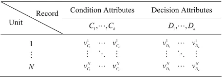
, Vr.If attribute sets R can be further broken down into condition attribute C and decision attribute D, and when it satisfies R C D C D , ,D, Information set can also be called a decision system or decision table (Table 1). If decision table contains only one decision attribute, it is called a single decision-making. Otherwise, it is called multi-decision.
2.1.2. Indiscernibility Relation
[image:2.595.309.538.657.737.2]Indiscernibility relation use ind X
represented and is an equivalence relation. U is divided into a finite number of equivalent set. It is indiscernibility between objects in each equivalent set. The first step of classification in the rough set is using ind X
to construct the basic set. ItTable 1. Decision system.
Condition Attributes Decision Attributes Record
Unit
1, , k
C C D1, ,Dn
1
N
1
1
1 1
k
k
C C N N C C
v v
v v
1
1
1 1
n
n
D D N N D D
v v
v v
is expressed as a mathematical model
, , ,
,
,
ind X x y U U a X f x a f y a ,
where X U X, .
2.1.3. Upper Approximation and Lower Approximation
Positive domain pos XR
or lower approximation of X is a set of elements which completely determined to clas- sify set X in U under R. It is defined as
:
R
pos X RX
Y U R Y X .Negative domain negR
X or Upper approximation of X is a set of elements which could not completely de- termined to classify set X in U under R. It is defined as
:
R
neg X RX
Y U R Y X .If RX RX , boundary bn XR
exists. Boundary is a set of elements which probably classify set X in U un- der R. It means the set neither completely determined to classify set X nor completely determined to classify set U X . It is defined as bn XR
RX RX .2.1.4. Dispensable and Independent
R is a set in equivalence relations. While r R , if
ind R ind R r , it is said r in R can be omitted. On the contrary, if ind R
ind R
r
, it is said r in R can be independent.2.1.5. Dependents and Significant of Attributes
Assume in decision system, positive domain pos XR
of decision attribute D under condition attribute C is di-vided by knowledge of C. It is defined as
C
X U D
pos D C X
. And dependent of attribute
C D means dependence of decision attribute D on
condition attribute C. It is defined as C
C
pos D DU
.
While C
D 1, it is said D is completely derivableunder C; while 0C
D 1, it is said D is partial de-rivable under C; while C
D 0, it is said D is notcompletely derivable under C. Dependent of attribute can decide significant of attribute. The usual practice is deleteing a attribute Ci and calculating the impact of positive domain under C. It is defined as
, 1
i i
C C C C C
i C D
C C
D D D
C
D D
.
2.1.6. Reduct and Core of Rough Sets
For decision system given, if RC is independent and
ind R ind C , it is said R is a reduct red
C of C.An attribute set maybe have various reduct. Intersection of reduct is said core of C, represented core
C
red C
. Core can be interpreted as the most important part of knowledge, can not delete while reduct.2.1.7. Decision Rule Having the Most Efficient
After calculations of reduct and core in decision system, rules can be extracted by the reduction of the decision system. The type of rules is if “characteristic value after reduction of sentence” then “a classification of decision attribute”. These rules express extracted knowledge from raw data.
2.2. Interpretive Structural Modeling (ISM)
Interpretive Structural Modeling (ISM) is proposed in 1976 by Warfield. The mathematical analysis transforms the relationship between the different types of elements into the associated constructor class diagram in a com- plex system [29]. While analyzing, using the Hierarchical Digraph in Graphic Theory describes the relationship between different types of elements. As a result, ISM transform fragmental and abstractive elements into the specific and comprehensive associated constructor class diagram in a complex system to clarify the structure of the complex situations [30].
While calculating, the relationship between the various elements must be arranged. Causality analysis table is established by binary matrix. Binary data of “1” and “0” means that the elements of related or unrelated. The ma- trix is represented by symbol A. To use Graphic Theory, the adjacency matrix A plus the unit matrix I becomes “contains its own causality matrix” represented by sym-bol B. Though B B 2B3Bn1Bn (Bn expresse B multiplied by n times), B is trasformed into reachable matrix represented by symbol T. It means T Bn. Finally, all the structural elements in the event are transformed into the associated structural hierarchy chart to obtain a distribution position of various structural elements [29].
In recent years, the studies of applying ISM in educa- tion are very much. Such as making structural graph of learning interest factors in mathematics, and proposing guidance programs for students of different learning [31], structured analysis of the teaching content [32], propos- ing learning path of concepts by combining students’ misconceptions and ISM structural graph of concepts [33].
3. Research Methods
In this section, researchers first do reliability test in order to ensure the data is quite reliable and then drew research procedures.
3.1. Reliability Test of Data
This paper took two fourth grade classes in the same school for example. The number of items was 24, the average of students of each class was 15, and the num- ber of concepts were 7. Before analyzing, the researchers first test reliability of students’ responses for two classes. The results showed that Cronbach’s α value of Class A is 0.854 and Cronbach’s α value of Class B is 0.849. These data represent high reliability.
3.2. Research Procedures
The study analyzed students’ misconception based on rough set theory and combined with ISM to compare students’ degree of two classes. Research structure was shown in Figure 1.
4. Results and Discussion
Based on research structure, this section divides into several parts. About problems, researchers analyze the structural graph of concepts based on ISM. About stu- dents’ responses of Class A and B, researchers analyze the SCD table, find common misconceptions, and then formulate the remedial decision-making. Finally, re- searchers compare students’ degree of two classes.
4.1. Production and Analyses of the Structural Graph of Concepts Based on ISM
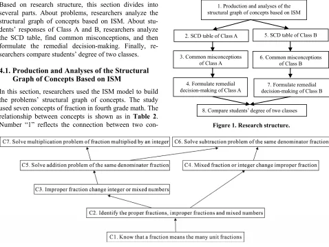
In this section, researchers used the ISM model to build the problems’ structural graph of concepts. The study used seven concepts of fraction in fourth grade math. The relationship between concepts is shown as in Table 2. Number “1” reflects the connection between two con-
cepts and the lack of connection is indicated as “0”. Researchers used ISM software to estimate a matrix calculation to obtain the causal linking structure between concepts which was the ISM structural graph of concepts (Figure 2). From Figure 2, structural graph of concepts has 5 layers, the lowest layer is the basic concept of this unit, and the top layer is the most difficult concept. When teachers teach this unit, there are three distinct teaching sequences, including C1 C2 C4 C6, C1 C2 C3 C5 C6 and C1 C2 C3 C5 C7.
4.2. SCD Table of Class A
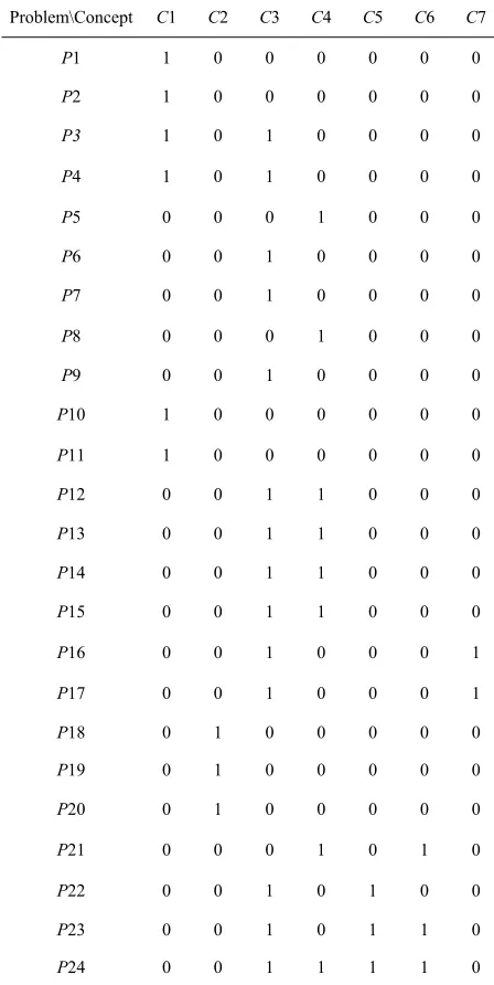
First, teachers judged the correlation between concept and problem. If there is a connection between concept and problem, then a corresponding column will reflect the number “1” and a lack of connection will show a “0” (Table 3). In this paper, students of two classes did same test, so they had the same problem-concept relationship.
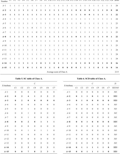
Students’ responses of Class A are shown in Table 4. “1” represents students answered correctly, “0” repre- sents students answered incorrectly. In this paper, if stu- dents’ score was lower than average score, researchers
1. Production and analyses of the structural graph of concepts based on ISM
2. SCD table of Class A
3. Common misconceptions of Class A
5. SCD table of Class B
6. Common misconceptions of Class B
7. Formulate remedial decision-making of Class B
8. Compare students’ degree of two classes 4. Formulate remedial
[image:4.595.58.536.369.727.2]decision-making of Class A
Figure 1. Research structure.
Table 2. Concept-concept relationship.
Concept\Concept C1 C2 C3 C4 C5 C6 C7
C1. Know that a fraction means the many unit fractions 0 1 1 1 1 1 1
C2. Identify the proper fractions, improper fractions and mixed numbers 0 0 1 1 1 1 1
C3. Improper fraction change integer or mixed numbers 0 0 0 0 1 1 1
C4. Mixed fraction or integer change improper fraction 0 0 0 0 0 1 0
C5. Solve addition problem of the same denominator fraction 0 0 0 0 0 1 1
C6. Solve subtraction problem of the same denominator fraction 0 0 0 0 0 0 0
[image:5.595.58.282.284.730.2]C7. Solve multiplication problem of fraction multiplied by an integer 0 0 0 0 0 0 0
Table 3. Problem-concept relationship.
Problem\Concept C1 C2 C3 C4 C5 C6 C7
P1 1 0 0 0 0 0 0
P2 1 0 0 0 0 0 0
P3 1 0 1 0 0 0 0
P4 1 0 1 0 0 0 0
P5 0 0 0 1 0 0 0
P6 0 0 1 0 0 0 0
P7 0 0 1 0 0 0 0
P8 0 0 0 1 0 0 0
P9 0 0 1 0 0 0 0
P10 1 0 0 0 0 0 0
P11 1 0 0 0 0 0 0
P12 0 0 1 1 0 0 0
P13 0 0 1 1 0 0 0
P14 0 0 1 1 0 0 0
P15 0 0 1 1 0 0 0
P16 0 0 1 0 0 0 1
P17 0 0 1 0 0 0 1
P18 0 1 0 0 0 0 0
P19 0 1 0 0 0 0 0
P20 0 1 0 0 0 0 0
P21 0 0 0 1 0 1 0
P22 0 0 1 0 1 0 0
P23 0 0 1 0 1 1 0
P24 0 0 1 1 1 1 0
set for students who need remedial teaching. Because average score is very close to 22 points, students who get 22 points were set. Finally, researchers judged the stu- dents who need remedial teaching are A−2, A−3, A−8,
A−14, and A−15.
In this paper, SCD table was formulated based on IS of rough set theory. SCD table is decision system, where S
represents the students; Condition attributes C represents concepts that are required learning in this unit; decision attribute D represents whether teachers do remedial teaching. Before formulating SCD table, SC table must first be needed (Table 5). SC table was obtained by combining problem-concept relationship (Table 3) and students’ responses of Class A (Table 4). It represents the number of incorrect responses in C1 to C7, respec- tively. For example: In Table 4, researchers can find A−5 had wrong response in P17, and C3 and C7 must be equipped to answer correctly. Thus, a corresponding column will reflect the number “1” in SC table of Class A.
In SC table, the number of some concepts that students answered incorrectly was a great difference. If doing rough set computing according SC table, the rules could not be obtained. In other words, it is unable to identify common misconceptions of the students. Thus in this paper, researchers assumed if students answered incur- rectly once at a certain concept, then it can be regarded as to got the wrong answer accidentally; if students an- swered incorrectly more than twice at a certain concept, then it can be regarded as to have the misconception. Based on the hypothesis, SC table was converted to SCD table (Table 6). In SCD table, students answered incor- rectly more than twice and then a corresponding column will reflect the number “1”; it will be showed a “0”, conversely.
The indiscernibility relation can be obtained according to the rough set theory. It is equivalence relation of S under the condition attributes. The result of the calcula- tion is as follows.
Table 4. Students’ responses of Class A.
Student\
Number P1 P2 P3 P4 P5 P6 P7 P8 P9 P10 P11 P12 P13 P14 P15 P16 P17 P18 P19 P20 P21 P22 P23 P24 Score
A−1 1 1 1 1 1 1 1 1 1 1 1 1 1 1 1 1 1 1 1 1 1 1 1 1 24
A−2 1 1 1 1 1 1 1 1 1 1 1 1 1 1 1 0 0 0 0 1 1 1 0 0 18
A−3 1 1 1 1 1 1 1 1 1 1 1 1 1 1 1 1 1 0 0 1 1 1 1 1 22
A−4 1 1 1 1 1 1 1 1 1 1 1 1 1 1 1 1 1 1 1 1 1 1 1 1 24
A−5 1 1 1 1 1 1 1 1 1 1 1 1 1 1 1 1 0 1 1 1 1 1 1 1 23
A−6 1 1 1 1 1 0 1 1 1 1 1 1 1 1 1 1 1 1 1 1 1 1 1 1 23
A−7 1 1 1 1 1 1 0 1 1 1 1 1 1 1 1 1 1 1 1 1 1 1 1 1 23
A−8 1 1 1 1 1 1 1 1 1 1 1 1 1 1 1 0 1 1 1 1 1 1 0 1 22
A−9 1 1 1 1 1 1 1 1 1 1 1 1 1 1 1 1 1 1 1 1 1 1 1 1 24
A−10 1 1 1 1 1 1 1 1 1 1 1 1 1 1 1 1 1 1 1 1 1 1 0 1 23
A−11 1 1 1 1 1 1 1 1 1 1 1 1 1 1 1 1 1 1 1 1 1 1 1 1 24
A−12 1 1 1 1 1 1 1 1 1 1 1 1 1 1 1 1 1 1 1 1 1 1 1 1 24
A−13 1 1 1 1 1 1 1 1 1 1 1 1 1 1 1 1 1 1 1 1 1 1 1 1 24
A−14 1 1 1 1 1 1 1 0 1 1 0 1 1 1 1 0 1 0 0 1 0 1 0 0 16
A−15 1 1 1 1 0 1 1 0 1 1 1 0 0 0 0 0 1 1 1 1 0 1 0 0 14
[image:6.595.56.538.115.734.2]Average score of Class A 21.9
Table 5. SC table of Class A.
C S\Attribute
C1 C2 C3 C4 C5 C6 C7
A−1 0 0 0 0 0 0 0
A−2 0 2 4 1 2 2 2
A−3 0 2 0 0 0 0 0
A−4 0 0 0 0 0 0 0
A−5 0 0 1 0 0 0 1
A−6 0 0 1 0 0 0 0
A−7 0 0 1 0 0 0 0
A−8 0 0 2 0 1 1 1
A−9 0 0 0 0 0 0 0
A−10 0 0 1 0 1 1 0
A−11 0 0 0 0 0 0 0
A−12 0 0 0 0 0 0 0
A−13 0 0 0 0 0 0 0
A−14 1 2 3 3 2 3 1
A−15 0 0 7 8 2 3 1
Table 6. SCD table of Class A.
C D
S\Attribute
C1 C2 C3 C4 C5 C6 C7 YES\NO
A−1 0 0 0 0 0 0 0 NO
A−2 0 1 1 0 1 1 1 YES
A−3 0 1 0 0 0 0 0 YES
A−4 0 0 0 0 0 0 0 NO
A−5 0 0 0 0 0 0 0 NO
A−6 0 0 0 0 0 0 0 NO
A−7 0 0 0 0 0 0 0 NO
A−8 0 0 1 0 0 0 0 YES
A−9 0 0 0 0 0 0 0 NO
A−10 0 0 0 0 0 0 0 NO
A−11 0 0 0 0 0 0 0 NO
A−12 0 0 0 0 0 0 0 NO
A−13 0 0 0 0 0 0 0 NO
A−14 0 1 1 1 1 1 0 YES
[image:6.595.238.528.440.733.2]
1
1, 2, 3, 4, 5, 6, 7, 8, 9, 10, 11, 12, 13, 14, 15
S ind C
A A A A A A A A
A A A A A A A
21, 4, 5, 6, 7, 8, 9, 10, 11, 12, 13, 14, 15 ,
2, 3, 14 S ind C
A A A A A A A
A A A A A A
A A A
31, 3, 4, 5, 6, 7, 9, 10, 11, 12, 13 ,
2, 8, 14, 15 S ind C
A A A A A A
A A A A A
A A A A
41, 2, 3, 4, 5, 6, 7, 8, 9, 10, 11, 12, 13 ,
14, 15 S ind C
A A A A A A A
A A A A A A
A A
5 61, 3, 4, 5, 6, 7, 8, 9, 10, 11, 12, 13 ,
2, 14, 15 S ind C S ind C
A A A A A A
A A A A A A
A A A
71, 3, 4, 5, 6, 7, 8, 9, 10, 11, 12, 13, 14, 15 ,
2 S ind C
A A A A A A A A
A A A A A A
A
To take the intersection from S ind C
1
to
7
S ind C , equivalence relations of S were obtained. It represents students of Class A were classified as six categories based on C1 to C7. The result of the calcula- tion is as follows.
1, 2, 3, 4, 5, 6, 7 1, 4, 5, 6, 7, 9, 10, 11, 12, 13 ,
2, 3, 8, 14, 15 S ind C
S ind C C C C C C C
A A A A A
A A A A A
A A A A A
If D is YES, to calculate equivalence relation based on conditional probability and indiscernibility relation can obtain the following results.
If
1 YES
2, 3, 8, 14, 15 X S D S
A A A A A
Upper approximation and the lower approximation are
1 1 2, 3, 8, 14, 15
RX RX A A A A A
Boundary is bn XR
1 Complement is
1 1, 4, 5, 6, 7, 9,
10, 11, 12, 13
S RX A A A A A A
A A A A
Similarly, if D is NO, to calculate equivalence relation based on conditional probability and indiscernibility rela-tion can obtain the following results.
If
2 NO1, 4, 5, 6, 7, 9, 10, 11, 12, 13
X S D S
A A A A A A
A A A A
Upper approximation and the lower approximation are
2 2
1, 4, 5, 6, 7, 9, 10, 11, 12, 13
RX RX
A A A A A A
A A A A
Boundary is bn XR
2 Complement is
2 2, 3, 8, 14, 15
S RX A A A A A
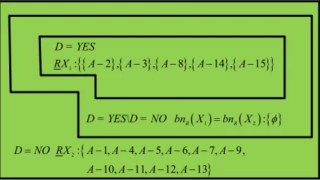
Results of the above calculations were drawn as Fig- ure 3. A−2, A−3, A−8, A−14, and A−15 who need reme- dial teaching can be determined in Class A; A−1, A−4,
A−5, A−6, A−7, A−9, A−10, A−11, A−12, and A−13 who need not remedial teaching can be determined in Class A. In addition, it is no sure whether remedial students in Class A.
4.3. Common Misconceptions of Class A
In order to find core of Class A, researchers do reduce of
D = YES\D = NO bn XR 1 bn XR 2 :
2: 1, 4, 5, 6, 7, 9,
10, 11, 12, 13 D NO RX A A A A A A
A A A A
D = YES
1: 2 , 3 , 8 , 14 , 15
[image:7.595.310.537.590.718.2]RX A A A A A
SCD table of Class A according to rough set theory. Core means common misconception of Class A. Three ways were provided as cross-validation while calculating.
First, researchers reduce data of SCD table. According to S ind C
1
, students could not be divided into two groups and S ind C
5
S ind C
6
, hence SCD table be simplified (Table 7).4.3.1. Deleting a Condition Attribute
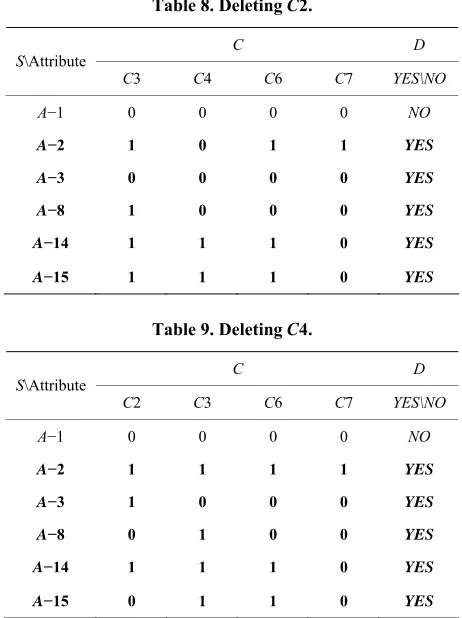
The first way is to delete a condition attribute in SCD summary table and to check whether there will be new conflicts. The following is the result of deleting and checking of each attribute. Researchers delete C2 and C4 as an example (Tables 8 and 9). After deleting C2, there was a new contradiction between A−1 and A−3. It repre- sented C2 could not be omitted.
1) After deleting C3, there was a new contradiction between A−1 and A−8. It represented C3 could not be omitted.
2) After deleting C4, there was no new contradiction. It represented C4 can be omitted.
3) After deleting C6, there was no new contradiction. It represented C6 can be omitted.
4) After deleting C7, there was no new contradiction. It represented C7 can be omitted.
By the analysis, C2 and C3 could not be omitted.
red C maybe were all sets containing C2 and C3. From SCD summary table of Class A, the student can be classified correctly and remedial teaching decision can be made whether just based on C2 and C3. Hence
red C C C2, 3 . It means core
C C C2, 3
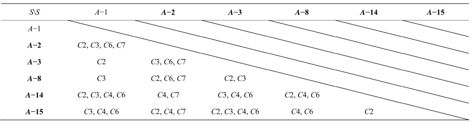
.4.3.2. Using Boolean Logic to Calculate Discernable Matrix
[image:8.595.307.538.88.397.2]The second way is to use Boolean logic to calculate discernable matrix. First, discernable matrix of Class A must be established. The researchers compared between students through the two-phase way and recorded differ- ent condition attributes in the matrix. For example, in
[image:8.595.57.287.591.735.2]Table 7, after comparing student A−1 and A−2, they have
Table 7. SCD summary table of Class A.
C D S\Attribute
C2 C3 C4 C6 C7 YES\NO
A−1 0 0 0 0 0 NO
A−2 1 1 0 1 1 YES
A−3 1 0 0 0 0 YES
A−8 0 1 0 0 0 YES
A−14 1 1 1 1 0 YES
A−15 0 1 1 1 0 YES
Table 8. Deleting C2.
C D S\Attribute
C3 C4 C6 C7 YES\NO
A−1 0 0 0 0 NO
A−2 1 0 1 1 YES A−3 0 0 0 0 YES A−8 1 0 0 0 YES
A−14 1 1 1 0 YES
A−15 1 1 1 0 YES
Table 9. Deleting C4.
C D S\Attribute
C2 C3 C6 C7 YES\NO
A−1 0 0 0 0 NO
A−2 1 1 1 1 YES A−3 1 0 0 0 YES
A−8 0 1 0 0 YES A−14 1 1 1 0 YES
A−15 0 1 1 0 YES
difference in C2, C3, C6, and C7. And so on, Table 10
can be completed.
By discernable matrix, the union of each student and other students can be calculated. It means that student maybe produce misconception in that concept. And then, to take the intersection of all union in the matrix is possible red
C of Class A. Result of the calculation is as follows.
red
2 3 6 7 2 3
2 3 4 6 3 4 6
3 6 7 2 6 7 4 7
2 4 7 2 3 3 4 6
2 3 4 6 2 4 6 4 6 2
C
C C C C C C
C C C C C C C
C C C C C C C C
C C C C C C C C
C C C C C C C C C C
red C C2C3 C4C7 C4C6
red C C2C3C4 C6C7
If attribute set is dependent, the smallest set of attrib-ute is red
C . Based on this rule,
7 4 6
3
S ind C S ind C S ind C S ind C
Table 10. Discernable matrix of Class A.
S\S A−1 A−2 A−3 A−8 A−14 A−15
A−1
A−2 C2, C3, C6, C7
A−3 C2 C3, C6, C7
A−8 C3 C2, C6, C7 C2, C3
A−14 C2, C3, C4, C6 C4, C7 C3, C4, C6 C2, C4, C6
A−15 C3, C4, C6 C2, C4, C7 C2, C3, C4, C6 C4, C6 C2
It can be obtained from indiscernibility calculation in SCD summary table of Class A while decision attribute
D is YES (The calculation process is as follows.). Hence
C4, C6, and C7 were not included in the red
C ,
red C C C2, 3 is obtained. It represented
core C C C2, 3 .
3
2, 8, 14, 15
S ind C A A A A
4
14, 15
S ind C A A
6
2, 14, 15
S ind C A A A
7
2
S ind C A
4.3.3. Calculating Significant of Condition Attributes
Using dependent of attribute can decide significant of attribute. The caculation of significant is removing a at-tribute Ci from C and finding the influencing degree of
Cpos D generated by C. Before calculating significant, dependent must be first calculated.
First, C
D must be calculated. And then C
D 1 is obtained. The calculation process is as follows.
1, 4, 5, 6, 7, 9, 10, 11, 12, 13 ,
2 , 3 , 8 , 14 , 15
S ind C
A A A A A
A A A A A
A A A A A
1, 4, 5, 6, 7, 9, 10, 11, 12, 13 ,
2, 3, 8, 14, 15
S ind D
A A A A A
A A A A A
A A A A A
1, 2, 3, 4, 5, 6, 7, 8, 9, 10, 11, 12, 13, 14, 15 Cpos D
A A A A A A
A A A A A
A A A A
Substituting formula of dependent,
15 1 15 C C pos D D S Then calculating S ind C C
1 , ,
S ind C C
7
individually. The calculation process are as follows.
11, 4, 5, 6, 7, 9, 10, 11, 12, 13 ,
2 , 3 , 8 , 14 , 15 S ind C C
A A A A A
A A A A A
A A A A A
21, 3, 4, 5, 6, 7, 9, 10, 11, 12, 13 ,
14 , 15 , 2 , 8 S ind C C
A A A A A A
A A A A A
A A A A
31, 4, 5, 6, 7, 8 9, 10, 11, 12, 13 ,
2 , 3 , 14 , 15 S ind C C
A A A A A A
A A A A A
A A A A
41, 4, 5, 6, 7, 9, 10, 11, 12, 13 ,
2 , 3 , 8 , 14 , 15 S ind C C
A A A A A
A A A A A
A A A A A
5 61, 4, 5, 6, 7, 9, 10, 11, 12, 13 ,
2 , 3 , 8 , 14 , 15 S ind C C S ind C C
A A A A A
A A A A A
A A A A A
71, 4, 5, 6, 7, 9, 10, 11, 12, 13 ,
2 , 3 , 8 , 14 , 15 S ind C C
A A A A A
A A A A A
A A A A A
To imitate the calculation of C
D , using of
1 , ,
7
S ind C C S ind C C , and S ind D
cal- culate individually pos DC
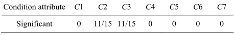
removing a attribute. Af- ter that, dependent of each attribute is obtained based on formula of dependent. Dependent of each attribute is shown in Table 11.Finally, the dependent of each attribute substitutes
formula of significance
, 1
i
C C i
C D
C D C
D
, re-
searchers got sequence of significance that is C1 = C4 =
C5 = C6 = C7 < C3 = C2. Significance of each attribute is shown in Table 12.
From Table 12, C1, C4, C5, C6, and C7 were redun- dant and could be removed. Researchers got
red C C C2, 3 , so core
C C C2, 3
.The calculation of the above three got the same results. It showed students of Class A had common misconcep- tion in C2 and C3 in fraction of unit. In Class A, teacher can do remedial teaching directly for two parts “Identify the proper fractions, improper fractions and mixed num- bers” and “Improper fraction change integer or mixed numbers”.
4.4. Formulate Remedial Decision-Making of Class A
By the analysis of Class A, it was seen C2 and C3 could not be omitted. In order to do the remedial teaching more efficiently, researchers extracted rules according two condition attributes. In this paper,
xP said that sets of students having same attribute value about attribute P.About Student A-1, reduct is C C20 30NO. The
calculation is shown as following.
2
1 1
1 1, 8, 15 1 ,
D
C D
A A
A A A A A
so C3 could not be omitted.
A1
C3
A1,A 3
A1
D, so C2 could not be omitted.About Student A−2 and A−14, reduct is
1 1
2 3 YES
C C . The calculation is shown as follow- ing.
Table 11. Dependent of each attribute.
Condition attribute C1 C2 C3 C4 C5 C6 C7
[image:10.595.57.286.701.736.2]Dependent 1 4/15 4/15 1 1 1 1
Table 12. Significant of each attribute.
Condition attribute C1 C2 C3 C4 C5 C6 C7
Significant 0 11/15 11/15 0 0 0 0
2
2 2, 3, 8, 14, 15
2 2, 3, 14 2 ,
D
C D
A A A A A A
A A A A A
so C3 could be omitted.
A2
C3
A2,A8,A14,A15
A2
D, so C2 could be omitted.About Student A−3, reduct is C21YES . The calculation is shown as following.
2
3 2, 3, 8, 14, 15
3 2, 3, 14 3 ,
D
C D
A A A A A A
A A A A A
so C3 could be omitted.
A3
C3
A1,A 3
A3
D, so C2 could not be omitted.About Student A−8 and A−15, reduct is C31YES.
The calculation is shown as following.
2
8 2, 3, 8, 14, 15
8 1, 8, 15 8 ,
D
C D
A A A A A A
A A A A A
so C3 could not be omitted.
A8
C3
A2,A8,A14,A15
A8
D, so C2 could be omitted.Take union of reduct of each student above, remedial decision-making of Class A obtained is the following two points:
1) If C2 = 1 or C3 = 1, then student needs remedial teaching.
Based on the ISM structural graph of concepts, C2is simpler than C3. Therefore, in the remedial process, teachers can adjust remedial instruction according to the students’ level. If students have a lower level, remedy of
C2 can be given first; if students have a higher level, remedy of C3 can be given directly.
2) If C2 0 and C7 0 , then student do not need remedial teaching.
4.5. SCD Table of Class B
Similarly, students’ responses of Class A are shown in
Table 13. “1” represents students answered correctly, “0” represents students answered incorrectly. If students’ score was lower than average score, researchers set for students who need remedial teaching. Researchers judged the students who need remedial teaching are B−1, B−8, and B−9.
Table 13. Students’ responses of Class B.
Student\
Number P1 P2 P3 P4 P5 P6 P7 P8 P9 P10 P11 P12 P13 P14 P15 P16 P17 P18 P19 P20 P21 P22 P23 P24 Score
B−1 1 1 1 1 0 1 1 1 1 1 1 1 1 1 1 1 0 1 1 1 1 0 0 0 19
B−2 1 1 1 1 1 1 1 1 1 1 1 1 1 1 1 1 0 1 1 1 1 1 1 1 23
B−3 1 1 1 1 1 1 1 1 1 1 1 1 1 0 1 1 1 1 1 1 1 1 0 1 22
B−4 1 1 1 1 1 1 1 1 1 1 1 1 1 1 1 1 1 1 1 1 1 1 1 1 24
B−5 1 1 1 0 1 1 1 1 1 1 1 1 1 1 1 1 1 1 1 0 1 1 1 1 22
B−6 1 1 1 1 1 1 1 0 1 1 1 1 1 1 1 1 1 1 1 1 1 1 1 1 23
B−7 1 1 0 1 1 1 1 1 1 1 1 1 1 1 1 1 1 1 1 1 1 1 1 1 23
B−8 1 1 1 1 1 1 1 1 1 1 0 1 1 1 1 0 1 0 0 1 0 0 1 0 17
B−9 1 1 0 1 1 1 0 1 1 0 0 1 0 1 0 1 1 0 0 0 0 0 0 0 11
B−10 1 1 1 1 1 1 1 1 1 1 1 1 1 1 1 1 1 1 1 1 1 1 1 0 23
B−11 1 1 1 1 1 1 1 1 1 1 0 1 1 1 0 1 1 1 1 1 1 1 1 1 22
B−12 1 1 1 1 1 1 1 1 1 1 1 1 1 1 1 1 1 1 1 1 1 1 1 1 24
B−13 1 1 1 1 1 1 1 1 1 1 1 1 1 1 1 1 1 1 1 1 1 1 1 0 23
B−14 1 1 1 1 1 1 1 1 1 1 1 1 1 1 1 1 1 1 1 1 1 1 1 1 24
B−15 1 1 1 1 1 1 1 1 1 1 1 1 1 1 1 1 0 1 1 1 1 1 0 1 22
Average score of Class B 21.5
Table 14. SC table of Class B.
C S\Attribute
C1 C2 C3 C4 C5 C6 C7
B−1 0 0 4 2 3 2 1
B−2 0 0 1 0 0 0 1
B−3 0 0 2 1 1 1 0
B−4 0 0 0 0 0 0 0
B−5 1 1 1 0 0 0 0
B−6 0 0 0 1 0 0 0
B−7 1 0 1 0 0 0 0
B−8 1 2 3 2 2 2 1
B−9 3 3 7 4 3 3 0
B−10 0 0 1 1 1 1 0
B−11 1 0 1 1 0 0 0
B−12 0 0 0 0 0 0 0
B−13 0 0 1 1 1 1 0
B−14 0 0 0 0 0 0 0
B−15 0 0 2 0 1 1 1
Class B (Table 13). It represents the number of incorrect responses in C1 to C7, respectively.
According previous mode, SC table was converted to SCD table (Table 15). In other words, if students an- swered incorrectly once at a certain concept, then it can be regarded as to get the wrong answer accidentally; if students answered incorrectly more than twice at a cer- tain concept, then it can be regarded as to have the mis- conception.
Similarly, the indiscernibility relation can be obtained according to the rough set theory. It is equivalence rela- tion of S under the condition attributes. The result of the calculation is as follows.
1
1, 2, 3, 4, 5, 6, 7, 8, 10, 11, 12, 13, 14, 15 ,
9 S ind C
B B B B B B B
B B B B B B B
B
2
1, 2, 3, 4, 5, 6, 7, 10, 11, 12, 13, 14, 15 ,
8, 9 S ind C
B B B B B B B
B B B B B B
B B
[image:11.595.57.282.435.732.2]Table 15. SCD table of Class B.
C D S\Attribute
C1 C2 C3 C4 C5 C6 C7 YES\NO
B−1 0 0 1 1 1 1 0 YES
B−2 0 0 0 0 0 0 0 NO
B−3 0 0 1 0 0 0 0 NO
B−4 0 0 0 0 0 0 0 NO
B−5 0 0 0 0 0 0 0 NO
B−6 0 0 0 0 0 0 0 NO
B−7 0 0 0 0 0 0 0 NO
B−8 0 1 1 1 1 1 0 YES
B−9 1 1 1 1 1 1 0 YES
B−10 0 0 0 0 0 0 0 NO
B−11 0 0 0 0 0 0 0 NO
B−12 0 0 0 0 0 0 0 NO
B−13 0 0 0 0 0 0 0 NO
B−14 0 0 0 0 0 0 0 NO
B−15 0 0 1 0 0 0 0 NO
3
2, 4, 5, 6, 7, 10, 11, 12, 13, 14 ,
1, 3, 8, 9, 15 S ind C
B B B B B
B B B B B
B B B B B
4 5 6
2, 3, 4, 5, 6, 7, 10, 11, 12, 13, 14, 15 ,
1, 8, 9
S ind C S ind C S ind C
B B B B B B
B B B B B B
B B B
7
1, 2, 3, 4, 5, 6, 7, 8, 9, 10, 11, 12, 13, 14, 15
S ind C
B B B B B B B B
B B B B B B B
To take the intersection from S ind C
1
to
7
S ind C , equivalence relations of S was obtained. It represents students of Class A were classified as five categories based on C1 to C7. The result of the calcula- tion is as follows.
1, 2, 3, 4, 5, 6, 7 2, 4, 5, 6, 7, 10, 11, 12, 13, 14 , 3, 15 ,
1 , 8 , 9
S ind C S ind C C C C C C C
B B B B B B
B B B B B B
B B B
If D is YES, to calculate equivalence relation based on conditional probability and indiscernibility relation can obtain the following results.
If X1
S D S
YES
B1,B8,B9
Upper approximation and the lower approximation are
1 1 1, 8, 9
RX RX B B B Boundary is bn XR
1 Complement is
1 2, 3, 4, 5, 6, 7, 10,
11, 12, 13, 14, 15
S RX B B B B B B B
B B B B B
Similarly, if D is NO, to calculate equivalence relation based on conditional probability and indiscernibility relation can obtain the following results.
If
2 NO
2, 3, 4, 5, 6, 7, 10, 11, 12, 13, 14, 15
X S D S
B B B B B B B
B B B B B
Upper approximation and the lower approximation are
2 2
2, 3, 4, 5, 6, 7, 10, 11, 12, 13, 14, 15
RX RX
B B B B B B B
B B B B B
Boundary is bn XR
1 Complement is
2 1, 8, 9
S RX B B B
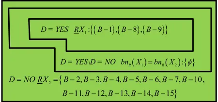
Results of the above calculations were drawn as Fig- ure 4. B−1, B−8, and B−9 who need remedial teaching can be determined in Class B; B−2, B−3, B−4, B−5,
B−6, B−7, B−10, B−11, B−12, B−13, B−14, B−15 who need not remedial teaching can be determined in Class B. In addition, it is no sure whether remedial students in Class B.
4.6. Common Misconceptions of Class B
In order to find core of Class B, researchers do reduct of SCD table of Class B again according to rough set theory. Core means common misconception of Class A. Simi-
D = YES RX1:
B1 , B8 , B9
D = YES\D = NO bn XR 1 bn XR 2 :
2 2, 3, 4, 5, 6, 7, 10,
11, 12, 13, 14, 15 D NO RX B B B B B B B
B B B B B
[image:12.595.311.536.609.715.2]larly, three methods were provided as cross-validation while calculating.
First, researchers reduce data of SCD table. Because
7
S ind C could not divide students into two groups and S ind C
4
S ind C
5
S ind C
6
, SCD table be simplified (Table 16).4.6.1. Deleting a Condition Attribute
The first way is deleting a condition attribute of SCD summary table and checking whether there will be new conflicts. The steps were the same as Class A. The fol- lowing results were obtained after calculation.
1) After deleting C1, there was no new contradiction. It represented C1 can be omitted.
2) After deleting C2, there was no new contradiction. It represented C2 can be omitted.
3) After deleting C3, there was no new contradiction. It represented C3 can be omitted.
4) After deleting C6, there was a new contradiction between B−1 and B−3. It represented C6 could not be omitted.
By the analysis, C6 could not be omitted. red
C maybe was all sets containing C6. From SCD summary table of Class B, it is easy to correctly classify students and to decide whether remedial teaching just only based on C6.Due to S ind C
4
S ind C
5
S ind C
6
, so red
C
C4 , C5 , C6
and core
C .4.6.2. Using Boolean Logic to Calculate Discernable Matrix
The second way is using Boolean logic to calculate discernable matrix. Similarly, discernable matrix of Class A must be established. The researchers compared be- tween students through the two –phase way and recorded different condition attributes in the matrix. And so on,
Table 17 can be completed.
By discernable matrix, the union of each student and other students can be calculated. And then, to take the intersection of all union in the matrix is possible
[image:13.595.59.286.614.735.2]red C of Class B. Result of the calculation is as fol- lows.
Table 16. SCD summary table of Class B.
C D S\Attribute
C1 C2 C3 C6 YES\NO
B−1 0 0 1 1 YES
B−2 0 0 0 0 NO
B−3 0 0 1 0 NO
B−8 0 1 1 1 YES
B−9 1 1 1 1 YES
red 3 6 2 1 2 3
2 3 6 1 2 3 6
2 6 1 2 6 1
C C C C C C C
C C C C C C C
C C C C C C
red C C1C2C3C6
If attribute set is dependent, the smallest set of attrib- ute is red
C . Based on this rule,
1 2 3
6
S ind C S ind C S ind C S ind C
it can be obtained from indiscernibility calculation in SCD summary table of Class B while decision attribute
D is YES (The calculation process is as follows.). Hence
C1, C2, and C3 were not included in the red
C . In addition to S ind C
4
S ind C
5
S ind C
6
, so red
C
C4 , C5 , C6
and core
C .
1 9
2 8, 9
3 1, 8, 9 6 1, 8, 9
S ind C B S ind C B B S ind C B B B S ind C B B B
4.6.3. Calculating Significant of Condition Attributes
To imitate the analysis of the Class A, using dependent of attribute can decide significant of attribute. Before calculating significant, dependent must be first calculated. Similarly, C
D must be calculated. And then
1 C D is obtained. The calculation process is as follows.
2, 4, 5, 6, 7, 10, 11, 12, 13, 14 , 3, 15
1 , 8 , 9
S ind C
B B B B B B
B B B B B B
B B B
2, 3, 4, 5, 6, 7, 10, 11, 12, 13, 14, 15 ,
1, 8, 9
S ind D
B B B B B B
B B B B B B
B B B
1, 2, 3, 4, 5, 6, 7, 8, 9, 10, 11, 12, 13, 14, 15 C
pos D
B B B B B B B B
B B B B B B B
Substituting formula of dependent,
15 1 15 CC
pos D D
S