2D-Shape Analysis Using
Conformal Mapping
The Harvard community has made this
article openly available.
Please share
how
this access benefits you. Your story matters
Citation
Sharon, E., and David Bryant Mumford. 2006. 2D-shape analysis
using conformal mapping. International Journal of Computer Vision
70(1): 55-75.
Published Version
doi:10.1007/s11263-006-6121-z
Citable link
http://nrs.harvard.edu/urn-3:HUL.InstRepos:3720034
Terms of Use
This article was downloaded from Harvard University’s DASH
repository, and is made available under the terms and conditions
applicable to Other Posted Material, as set forth at http://
2D-Shape Analysis Using Conformal Mapping
E. SHARON AND D. MUMFORD∗
Division of Applied Mathematics, Brown University, Rhode Island, Providence, 02912,
Received April 26, 2005; Revised November 9, 2005; Accepted November 9, 2005
First online version published in June, 2006
Abstract. The study of 2D shapes and their similarities is a central problem in the field of vision. It arises in
particular from the task of classifying and recognizing objects from their observed silhouette. Defining natural distances between 2D shapes creates a metric space of shapes, whose mathematical structure is inherently relevant to the classification task. One intriguing metric space comes from using conformal mappings of 2D shapes into each other, via the theory of Teichm¨uller spaces. In this space every simple closed curve in the plane (a “shape”) is represented by a ‘fingerprint’ which is a diffeomorphism of the unit circle to itself (a differentiable and invertible, periodic function). More precisely, every shape defines to a unique equivalence class of such diffeomorphisms up to right multiplication by a M¨obius map. The fingerprint does not change if the shape is varied by translations and scaling and any such equivalence class comes from some shape. This coset space, equipped with the infinitesimal Weil-Petersson (WP) Riemannian norm is a metric space. In this space, the shortest path between each two shapes is unique, and is given by a geodesic connecting them. Their distance from each other is given by integrating the WP-norm along that geodesic. In this paper we concentrate on solving the “welding" problem of “sewing" together conformally the interior and exterior of the unit circle, glued on the unit circle by a given diffeomorphism, to obtain the unique 2D shape associated with this diffeomorphism. This will allow us to go back and forth between 2D shapes and their representing diffeomorphisms in this “space of shapes”. We then present an efficient method for computing the unique shortest path, the geodesic of shape morphing between each two end-point shapes. The group of diffeomorphisms of S1acts as a group of isometries on the space of shapes and we show how this can be
used to define shape transformations, like for instance ‘adding a protruding limb’ to any shape.
Keywords: group of diffeomorphisms, group of shape transformations, shape representation, metrics between shapes, conformal, Riemann mapping theorem, Weil-Petersson metric, geodesic, fingerprints of shapes
1. Introduction
Many different representations for the collection of all 2D shapes1, and many different measures of
similar-ity between them have been studied recently (Hildreth, 1984; Kass et al., 1988; Ullman, 1989; Amit 1991; Yuille, 1991; Sclaroff and Pentland, 1995; Kimia et al.,1995; Geiger et al.,1995; Gdalyahu and Weinshall, 1999; Basri et al.,1998; Belongie et al.,2002;
Sebas-∗Research was supported by NSF grants DMS-0074276 and IIS-0205477.
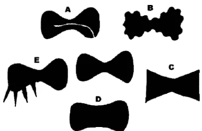
Figure 1. All the figures A, B, C, D and E are similar to the middle one, but they differ in different ways. Which shapes should be considered closer may depend on context. This illustration is due to B. Kimia.
Representing shapes in a simple way for classifi-cation is difficult because of two things: on the one hand, the set of all shapes is inherently infinite dimen-sional and, on the other hand, it has no natural linear structure. More precisely, the first assertion means that if we map every shape to a point of Rn by
assign-ing to it n features, there will always be many distinct shapes on which all these features coincide. You can-not capture all the variability of a shape in a finite set of features. The second assertion means that there is no vector space structure on the set of all shapes, no way of adding, subtracting and multiplying by scalars in this set which satisfies the vector space axioms2. So if we use an infinite number of features to describe shapes, such as all its moments or all its Fourier coef-ficients, then although we get a representation of the set of shapes in a vector space, there will be sequences of moments or Fourier coefficients which do not come from any shape. The upshot is that the set of all shapes is mathematically rather complicated. We feel this is the deep reason why shape classification algorithms in the literature have been less than perfectly satisfactory. Although the set of shapes is nonlinear and infinite dimensional, this does not prevent it from having its own geometry. The first step towards analyzing its ge-ometry is to endow this set with a metric, a numerical measure of the difference between any 2 shapes. Many metric approaches for the classification of shapes have also been suggested. The Hausdorff distance is perhaps the best known: this is a ‘sup’ or so called L∞norm. One can also take the area of the symmetric difference of the interiors of the 2 shapes: this is a L1type norm,
gotten by a simple integral. We may also measure in some way the difference of the orientations as well as the locations of the 2 shapes: these are first derivative
norms. One can play with these alternatives and work out which shapes in Fig. 1 are closer to the central shape in which metric.
In our method of representing shapes, every shape will define a sort of ‘fingerprint’, which is a diffeomor-phism of the unit circle to itself. Such a diffeomordiffeomor-phism is given by a smooth increasing function f :R→R which is differentiable and satisfies f (x+2π)=f(x)
+2πand two functions f1, f2define the same
diffeo-morphism if f1(x)≡f2(x)+2πn. The group of such
diffeomorphisms will be denoted by Diff(S1). The
con-struction is based on the existence of a conformal map-ping from the interior of any shapeto the interior of the unit disk via the Riemann mapping theorem. Like all conformal maps, it preserves the angles between any two intersecting curves and, moreover, it is unique up to composition with a M¨obius-transformation ambiguity. More precisely, we will show that every simple closed curve in the plane defines an equivalence class of diffeomorphisms f. These equivalence classes are the right cosets of these diffeomorphisms modulo the three dimensional subgroup of M¨obius maps3
PSL2(R), namely the maps from the complex unit circle
{z|z| =1}to itself given by z→(az +b)/( ¯bz+ ¯a). This set of equivalence classes is then written as the
quotient Diff(S1)/PSL2(R). In this assignment, two
shapes1,2 define the same diffeomorphism only
when one shape is gotten from the other by a trans-lation and scaling, i.e. 2 = a ·1 +(b,c). If S
is the set of 2D shapes and H is the group of maps (x,y)→(ax+b,ay+c), then the result of this
con-struction is a bijection between the two quotient sets:
Diff(S1)/PSL2(R)∼=S/H.
shapes by composing the coset representing them by a diffeomorphism on the left and this transformation will preserve the WP distance, take geodesics to geodesics and hence change the above morphing between any two shapes into the morphing between the transformed shapes.
It is essential in this framework to be able to move back and forth computationally between 2D shapes and the diffeomorphisms representing them. Moving from a given shape into the diffeomorphism representing it can be done by computational implementations of the Riemann mapping theorem. Several approaches to this exist in the literature, see3.1. Perhaps the most effec-tive way is by using a numerical implementation of the Schwarz-Christoffel formula, applied to a polygon that tightly approximates the shape (Driscoll, 1996). But going back from the diffeomorphism to the shape is a new computational challenge, known as the “welding” problem. It involves the construction of two conformal maps, one defined inside the unit circle and one out-side, which differ on the unit circle by the given diffeo-morphism. In this paper, we will give two approaches to computing the solution of welding problem. Having this transformation between the space of shapes and the group of diffeomorphisms, we then go on to compute geodesics in the WP-metric. We do this by computing the geodesics in the coset space Diff(S1)/PSL2(R) and
then using welding to move this into a morphing of two plane shapes.
2. Shapes as Diffeomorphisms of the Circle
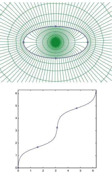
In this paper, by a “shape” we mean a simple closed smooth curve in the plane. Smooth means having derivatives of all orders (i.e. being C∞), and simple means that the curves do not intersect themselves. Ev-erything is based on the Riemann mapping theorem which states that it is possible to map the unit disc conformally to the interior of any such shape4. The conformal transformation is unique up to any preced-ing M¨obius transformations mapppreced-ing the unit disc to itself (that is, maps of the form z→(az+b)/( ¯bz+¯a)). Conformal means that the infinitesimal angle between each two crossing curves is equal to the infinitesimal angle between the transformed curves. The nature of these mappings is shown in Fig. 2, where the im-age of the radial grid on the unit disc (made out of concentric circles and lines through the origin) under this map is shown. Note that the image curves remain perpendicular.
0 1 2 3 4 5 6
[image:4.595.311.524.125.459.2]0 1 2 3 4 5 6
Figure 2. On the top, the conformal parametrization of the interior and exterior of an ellipse given by the Riemann mapping theorem, shown by plotting the images under−and+of circles around the origin and radial lines. On the bottom, the ‘fingerprint’. The circled points on the 2 figures are corresponding points. Note the large derivative of the fingerprint at the pointsθ=0,πcorrsponding to the ends of the major axis and the small derivative at the points
θ=π/2, 3π/2 corresponding to the ends of the minor axis.
2.1. Shapes to Diffeomorphisms
In this whole paper, we associateR2with the complex
planeCand hence we denote planar points by complex numbers u+iv. We often want to add in the ‘point at infinity’; adding this in, we get the extended complex plane, also called the Riemann sphere and denoted by
ˆ
C=. C∪ {∞}
Further, we denote the unit disc {z | |z| ≤ 1}by
− and the infinite region outside or on the unit disc
{z| |z| ≥1}(including∞) by+. Observe that using the transformation z→1/z we can identify+with
−. For every simple closed curveinCwe denote
Figure 3. The conformal map f, as described in Sec.2.2, maps the two halves of the z-sphere divided by the unit circle (left) onto the two parts of the w-sphere divided by(right), correspondingly, such that f−(z)=f+(ϕ(z)) on |z|=1.
denote by+its union with the infinite region outside
(including ∞). We can think of − and+ as a partition of the Riemann sphere into two parts along (see Fig.3).
Then by the Riemann mapping theorem, for all there exists a conformal map
−:−→−,
unique up to replacing−by−◦A for any M¨obius
transformations A :−→−, A=(az+b)/( ¯bz +
¯a). That is, for every two conformal maps(1)−, (2)− :
−→−we have that(2)−−1◦(1)− =A, where A is
a M¨obius map.
This works for+and+too as the point at infinity is no different from other finite points. Spelling this out, under 1/z, is transformed into the inverted simple closed curveso that+is identified with the interior
− of. Thus we can apply the Riemann mapping
theorem to get a from − and −. Composing this conformal map with inverse on both sides, i.e.
+(z) =1/(1/z), we get a conformal map of the
exteriors
+:+→+.
+ is also unique up to M¨obius transformations as above. But now we can do better with+: we take the unique M¨obius map A so that, replacing+ by+◦ A, we achieve the extra normalization that+carries
∞to∞, and that its differential carries the real posi-tive axis of the-plane at∞to the real positive axis of the-plane at∞. Thus, we eliminate the M¨obius ambiguity of + for every, and make+ unique. An example of this construction is shown at the top in Fig.2, where the curveis an ellipse.
The goal of this construction is to define the map
.=+−1◦−,
which it is defined on the unit circle S1. (Note that
−(S1)=, and
+−1()=S1.) : S1 → S1 is a diffeomorphism, which can be thought of as a peri-odic, real-valued function from [0, 2π] to [0, 2π], hav-ing a positive derivative everywhere. is a uniquely-identifying fingerprint of the shape. The fingerprint of the ellipse is also shown in Fig.2.
From the M¨obius-transformation ambiguity left in
− we can see that by the construction of every
simple closed curve induces a diffeomorphism : S1 → S1, which is unique up to composing on the
right by a diffeomorphism ˜A : S1→ S1coming from
the restriction to S1of any M¨obius transformation A :
−→−.
If, as in the introduction, we denote the coset space5 by Diff(S1)/PSL2(R) and we denote the space of sim-ple closed smooth curvesbyS, then our construction of gives us the ‘fingerprint’ map:
S →Diff(S1)/PSL2(R).
2.2. Diffeomorphisms to Shapes: Welding
Remarkably, this map is nearly a bijection. In fact, every coset ·PSL2(R) comes from some shape
and two shapes1,2give the same coset if and only
if they differ by a translation and scaling. If S is the quotient of shapes modulo translations and scalings, the final result is
S∼=Diff(S1)/PSL2(R). (1) To obtain, −and+corresponding to any coset, we first pick anyin the coset. The ‘high level’ way of findingis to construct an abstract Riemann surface
X by ‘welding’+ and−using the map to glue their boundaries together and apply the result that any Riemann surface which is topologically a 2-sphere – like X – is, in fact, conformally isomorphic to ˆCvia some map. Then ± are just the restrictions of to ± and the shape is nothing but the image of the unit circle in the welded surface X under. This construction is illustrated in Fig.3.
L. Bers [9, p., 10]. We sketch the proof without details. We use the standard abreviations:
fz =
1
2( fx−i fy), f¯z= 1
2( fx+i fy). The theorem states that for any c<1 and any complex valued functionµ(z) with|µ(z)| ≤c (called a Beltrami differential), the partial differential equation:
F¯z=µFz,
has a complex valued solution6. We get theµfrom as follows. First define G :−→−by:
G(r eiθ)=r ei(θ).
Then letµ = G¯z/Gz on− (one can readily check
that this works out to be eiθ1−
1+) andµ=0 on+.
With thisµ, solve the above equation for the function
F. Becauseµ=0 on+, F must be a conformal map on+, hence it extends to∞and we can normalize it to have positive real derivative there. Let + be
F on +. Note that G satisfies the equation on −
and, by standard arguments, any other solution there is G followed by an analytic function (that is a map with complex derivatives but which is not everywhere conformal because they can be zero). So let−be the analytic function F ◦ G(−1) on−. Then− ◦ G≡
+on the unit circle, as required. 2.3. Shapes with Base Points
We have now seen that shapes, up to scaling and translation, are represented by cosets·PSL2(R) ⊂
Diff(S1). An important variant of this representation
concerns shapes with base points, that is pairs {,
P} where P is a point in the interior of . The re-sult is that shapes with base points are represented by cosets · ROT(S1) ⊂Diff(S1) where ROT(S1) is
the group of rotationsθ→θ +φof the circle. Note that ROT(S1) ⊂PSL2(R) as the rotation through an-gleφis given by the map z→ (az+b)/( ¯bz+¯a) for
a =eiφ/2,b=0.
This representation is a simple extension of what we have already seen: having a base point P in the interior of the shapeallows one to normalize the conformal map−so that−(0)=P. This fixes−up to right multiplication by a rotation, henceis also determined up to such a right multiplication. This state of affairs
is often depicted by a ‘commutative diagram’:
Diff(S1)/R O T (S1)∼= {,P}/H
↓ ↓
Diff(S1)/PSL2(R) ∼= {}/H
where the vertical arrows denote the maps given by (i) passing from the small cosets mod ROT to the larger cosets mod PSL; and (ii) passing from a shape with base point to a shape without base point.
Closely related to this is the following remark: if a coset·PSL2(R) represents the shape, then the
cosets A◦·PSL2(R), for various M¨obius maps A∈ PSL2(R) represent the shapes B() for those complex
M¨obius maps B ∈ PSL2(C) such that B−1(∞) lies
outside. Recall that complex M¨obius maps are the maps of the extended complex plane given by z → (az+b)/(cz+d). To see this, use the definition =
−1
+ ◦−. Then multiplyingon the right by A is the
same as replacing+by+ ◦ A. Now+ ◦A is a
good conformal map of the exterior of the unit circle onto the exterior of , only it doesn’t have the right normalization any more as it doesn’t carry∞to∞. In fact, Q=+(A(∞)) is some point in the exterior of. Choose a complex M¨obius map B so that B−1(∞)= Q. Further require that B−1carry the positive real axis tangent direction at ∞ to the tangent direction at Q which is the image of the positive real direction under
+◦A. Then B◦+◦A is fully normalized, carrying
∞ to itself and carrying the postive real direction at
∞ to itself. Thus + =B ◦ + ◦ A and − = B
◦ − are the exterior and interior conformal maps
for the shape B(). Thus the fingerprint of B() is
=(
+)−1◦−=A◦−1+ ◦−=A◦. 2.4. The Homogeneous Structure ofS
Any group G operates, of course, on any coset space
G/H by left multiplication, hence, as a result of the
above construction, Diff(S1) operates on the space of
shapes S. A concrete way of defining this action is this: to transform any ∈ S by a group element , we construct the conformal map + : + → + hence we get the map=+◦◦−1+ fromto itself. Then we use the same welding trick by cutting open ˆC along and rewelding it with the map . The result can be conformally mapped to the extended sphere, takingto a new curve. This way we get a
3. Computing Shapes from Diffeomorphisms and Vice Versa
3.1. Schwarz-Christoffel: From Shapes to Diffeomorphisms
There seem to be three published methods of comput-ing the conformal mappcomput-ing from the unit disk to the interior of a simple closed curve:
1 using the Schwarz-Christoffel formula, developed by Tobin Driscoll, cf. http://www.math.
udel.edu/∼driscoll/SC and Driscoll and
Trefethen (2002).
2 the method of circle packing, developed by Kenneth Stephenson, cf. http://www.math.
utk.edu/∼kens/ and Stephenson (1989)
3 the ‘zipper’ algorithm of Donald Marshall,
cf. http://www.math.washington.edu/
∼marshall/zipper.html.
The Schwarz-Christoffel method is like this: start by approximatingby a polygon. Let z be the complex coordinate in the unit disk, and let{ai}be the points
on the unit circle which will map to the vertices of the polygon and let{παi}be the angles of the polygon at
these vertices. Then for some C1, C2:
(z)=C1
z
0
i
(z−ai)αi−1d z+C2.
For instance, if the polygon is a square, then the con-formal map of the unit disk to its interior is given by the elliptic integral:
(z)=C1
z
0 d z
√
1−z4 +C2.
This method has been implemented in the excellent package ‘sc’ by Tobin Driscoll (cited above), based on joint work with L.N. Trefethen (1996). The key problem is that one is usually given only the points
(ai) and must compute{ai}at the same time as.
Moreover, they are non-unique as, for any M¨obius map
A, =◦ A,ai = A−1(ai) are equally good
solu-tions. The program allows you to specify the point
(0) ∈ Int() to get the best looking and best be-haved solution. We use this package for our examples in Section4below.
3.2. From Diffeomorphisms to Shapes: The First Method of Welding
3.2.1. Reducing Welding to Coupled Elliptic Bound-ary Value Problems. Setting the equations for the conformal map f (see Fig. 3). We consider− and
+ as a partition of the Riemann sphere into two
parts along the unit circle , and − and + as a partition of the Riemann sphere into two parts along
, as explained in Sec.2.1(see Fig.3). We associate the complex-plane variable z with the-sphere, and the complex-plane variable w with the-sphere. We will assume that 0 −in order to normalize the map
− as well as+ by asking that−(0) =0. Given
a diffeomorphism ϕ : → , we seek a function
f(z) from the z-sphere minus the unit circle to the w-sphere, complex analytic on|z|<1 with boundary values f||z|=1 =f−, and complex analytic on|z| >1
with f||z|=1=f+, such that f (0)=0, f (∞)= ∞
f−(z)= f+(ϕ(z)) |z| =1 (2)
Defining g, a function of f which is more convenient to compute. Note that f (z)/z has finite non-zero
lim-iting values at 0 and∞, hence it has a single-valued logarithm in−and+. Thus we may define g(u) by
log
f (eu)
eu
=g(u),u∈C−iR (3) so that g(u+2πi)≡g(u).
Now,
Re(u)→ −∞ ⇒ |eu| →0 ⇒ f (eu)≈c
1eu ⇒g(u)≈log c1,
(4) and
Re(u)→ ∞ ⇒ |eu| → ∞
⇒ f (eu)≈c2eu ⇒g(u)≈log c 2,
(5) for some constants c1and c2. Without loss of generality,
we can replace f by c2−1f so that c2=1, and g(u)≈0
as Re(u)→ +∞.
We define : R → R, satisfying (θ +2π) =
(θ)+2π byϕ(eiθ)=ei(θ).Then, g−(iθ)=log( f−(eiθ))−iθ
=log( f+(ϕ(eiθ)))−iθ=log( f+(ei(θ))−iθ
Thus we get a new welding condition on the imagi-nary axis
g−(iθ)=g+(i(θ))+i ((θ)−θ). (7) Note that if Eq.7holds atθ then it also holds atθ + 2π.
Setting the equations for g’s imaginary part k. (h is then known from k.) Now let
g(u)=h(u)+i k(u), (8) where h, k are real. Then,
h,k harmonic if Re(u)<0,Re(u)>0
h,k→0 if Re(u)→ +∞
h,k→suitable if Re(u)→ −∞ constants
h,k periodic if u→u+2πi.
(9)
Furthermore, from Eq.7we get that
h−(iθ)=h+(i(θ))
k−(iθ)=k+(i(θ))+(θ)−θ. (10) By the Cauchy-Riemann equations, if u=s+iθ, we have for s<0, s<0 that
∂h
∂θ = − ∂k
∂s,
∂h
∂s =
∂k
∂θ. (11)
For s=0 this gives
−∂∂k−
s =
∂h−
∂θ =(θ) ∂h+
∂θ = −(θ) ∂k+
∂s . (12)
Thus, we can conclude the following conditions on k
k harmonic on s<0, s>0
k periodic w.r.t.θ→θ+2π
k→0 if s→ ∞, k→c if s→ −∞
k−iθ=k+i(θ)+(θ)−θ on s=0
∂k−
∂s iθ =(θ) ∂k+
∂si(θ) on s=0,
(13)
[image:8.595.306.527.128.218.2]for some real constant c which comes implicitly from the equations. Note that Eq.13is in fact an equation for a real function k, of the two real variables s andθ. Having solved it for k=k(s,θ) we get h=h(s,θ) as
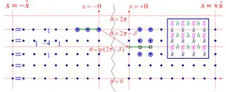
Figure 4. The (si,θj) k-grid on the (s,θ) plane. In blue over
the grid points, a schematic sketch of the three types of equations involved in the numeric solution of k, as described in Sec.3.2.2: the zero derivatives at the external boundaries (s= ±ˆs), described by the equal signs (Neuman boundary conditions), the template of the Laplacian mask applied to internal grid points (s= ±0,±ˆs), and the 9 grid points (circled) involved in the internal boundary condition for every internal-boundary grid point (s= ±0). The square inset demonstrates the three staggered grids, for the functions k, h and g. Every grid point is represented by the corresponding letter.
the conjugate function of k, via the Cauchy-Riemann relations in Eq.11.
f is then known from k and h. From Eq.3and Eq.8 we get that
f (es+iθ)=eh(s+iθ)+i (k(s+iθ)+θ). (14) Sinceis given by f(θ)|s=±0, we have that h(θ)|s=±0
and k(θ)|s=±0 describe the magnitude and angle,
re-spectively, of the complex-plane vectors delineating as a periodic function ofθ.
3.2.2. Solving the Elliptic Problem Numerically
Given a diffeomorphism , we solve Eq.13 for the
θ-periodic function k=k(s,θ) on the plane branchθ
∈ [0, 2π] and−∞ <s<∞. We conveniently set three different, staggered grids on (s,θ), with uniform meshsizeδ >0 for the three functions k, h and g (see the square inset in Fig.4). In practice, we cut off the s direction into−ˆs ≤s ≤ ˆs, for some ˆs >0, at which the values of k, h and g already converge to constants (cf. Eq.9). Solving for k on the k-grid, we use Eq.11 to compute h on the h-grid, and interpolating both to get g on the g-grid. It is the values of g on s = ±0 that fix the resulting curve. In practice, having k, we directly compute h on s= ±0, at the k-grid points, as explained at the end of Sec.3.2.2.
Solving for k: setting the s-grid and three types of numerical equations (see Fig. 4). Solving for
k(s, θ), we define the (si, θj) k-grid, by indexing
with i,j ∈ N an s-grid: si ∈ {−ˆs,(−ˆs + δ),
−δ)}(for which the index j applies periodically). We set three different types of equations.
Setting the Laplacian-mask equations. First we have
the basic simplest second-order discretization of the Laplace equation holding for every internal point, k being harmonic, that is:∀j and∀si= ±ˆs,±0 we have
0=δ12(−4k(si, θj)+k(si−1, θj)+k(si+1, θj) +k(si, θj−1)+k(si, θj+1))
(15)
Setting the Neuman-boundary-condition equations.
Second, accounting for k’s convergence to constants at
s= ±∞, we set Neuman boundary conditions at the external boundaries si = ±ˆs
k(−ˆs, θj)=k(−ˆs+δ, θj) ∀j k(ˆs, θj)=k(ˆs−δ, θj) ∀j
(16)
Setting the internal-boundary-condition (welding) equations. Third, we have the k-value, and k-derivative
pair of welding equations from Eq. 13, between the internal boundaries s= −0, associated with k−, and
s= +0 associated with k+.
For every j we will associate one such pair of equa-tions with every value k(−0, θj), and similarly with
every value k(+0,θj). We separate the equations for k− from those for k+ because the values of(θj)
in-volved in the equation for k(−0,θj) do not necessarily
fall on some grid lineθ˜j, sinceis a continuous
weld-ing diffeomorphism that does not typically sendθjinto
some other grid lineθ˜j. (Symmetrically, when focus-ing on the pair of weldfocus-ing equations for k(+0,θj) we
may have that−1(θj) is not a grid line.)
For every grid lineθjwe use the following
second-order discretizations for ∂∂ks±
∂k
∂s|(−0,θ) =
3
2δk(−0, θ)− 2
δk(−0−δ, θ) +1
2δk(−0−2δ, θ)+O(δ
2),
(17)
and
∂k
∂s|(+0,) = −
3
2δk+|(+0,)+ 2
δk|(+0+δ,)
−1
2δk|(+0+2δ,)+O(δ
2).
(18)
To replace the first term on the right, k|(+0,(θj)),
we may simply use the value of k at the grid point
(−0, θj), via the k-value welding equation from
Eq.13
k+|(+0,(θj))=k(−0, θj)−(θj)+θj. (19)
The other two values of k participating in Eq.18may each be simply interpolated from the nearest three grid points along theθ-direction. We use three such values to keep an approximation of orderδ2. More precisely,
for every s-column, and specifically for s= +0 +δ and s= +0+2δ, we can write the exact interpolation relations
k|(s,)=
(−θj2)(−θj3)
(θj1−θj2)(θj1−θj3)
k|(s,θj1)+O(δ
2 )
(−θj1)(−θj3) (θj2−θj1)(θj2−θj3)
k|(s,θj2)+
(−θj1)(−θj2)
(θj3−θj1)(θj3−θj2)k|(s,θj3),
(20)
whereθj1,θj2andθj3are the closest grid points to.
Substituting Eq. 19 and Eq. 20 in Eq. 18 we get from the last equation in Eq.13an equation between exactly 9 grid values. We associate this equation with the unknown k(−0,θj). A similar equation is associated
with k(+0,θj) for everyθj. Together with Eq.15and
Eq.16we have thus associated one equation with every grid point (si,θj). See Fig.4for exemplifying the three
different types of equations.
Regularizing the system of equations for k. Notice
however that the solution is still not uniquely fixed. Adding a constant to any solution of this system will keep it a solution still. Thus the system is singular. So we first need to add one more equation that will determine that constant. Recalling that k→0 as s→
∞(cf. Eq.9), a natural numerical equivalent condition would be thatθ2=0π k(∞, θ)=0, and in its descretized form
δ
j
k(ˆs, θj)=0. (21)
of the k-derivative welding equations, although other choices could be made as well.
Having computed k we compute h and then g, on
s= −0. Having computed the values of k over the k-grid we note that in order to get the resulting shape we only need the values of g(s,θ) and hence of h(s,θ) at either one of the internal boundaries s= ±0. We can use a discretized version of the first Cauchy-Riemann equation presented in Eq.11in order to approximate
∂h
∂θ on s= ±0, at exactly midpoints between the k-grid
points. Specifically we write
h(−0, θj+1)−h(−0, θj)
δ = −1
2
∂
k
∂s|(−0,θj+1)+
∂k
∂s|(−0,θj)
+O(δ2), (22)
where∂∂ks(−0,θ
j+1)and
∂k
∂s(−0,θj)were already computed
during the process of computing k, via Eq.17. We can easily integrate the values {h(−0, θj)}j out of their
differences computed in Eq.22, up to a global additive constant that does not matter in terms of the result-ing.
From{k(−0,θj)}jand{h(−0,θj)}jwe have{g(−0,
θj)}jvia Eq.8, and can get{f(−0,θj)}jvia Eq.3, and
eventually.
3.3. A Second Method of Welding
The second algorithm is based on the Hilbert trans-form. Recall that for functions on the real line, the Hilbert transform is convolution with the singular kernel 1/x and that it multiples the fourier transform of
the function by−i·sign(ξ). In our case, we are dealing with functions on the circle and the modified Hilbert transform is convolution with ctn(θ/2) or, equivalently, multiplication of the fourier coefficients by−i·sign(n). For any function f ∈ L2(S1), let H( f ) be its Hilbert
transform in this sense.
Now consider the function f+ as above. It is mero-morphic on{|z| ≥1} ∪ ∞and with a simple pole and positive real derivative at∞, hence it has an expansion:
f+(z)=bz+a0+a1z−1+a2z−2+ · · ·, b>0. Sinceis only defined up to scalings, we can normalize so that b=1. Thus, on the unit circle:
f+(eiθ)=eiθ+ n≥0
ane−i nθ.
Let F(θ)=f+(eiθ). Then
i H (F )(θ)=2eiθ+a0−F (θ).
On the other hand, we know that f−is holomorphic on
{|z| ≤1}, so it has the expansion:
f−(z)=c0+c1z+c2z2+ · · ·.
Since f−(eiθ)=F((θ)), we get:
i H (F◦)(θ)=(F◦)(θ)−c0.
Thus, by subtraction, we get:
i H (F◦)◦(−1)−i H (F )=2F−(a0+c0)−2eiθ.
We may replace F by F−a0+c0
2 sinceis only defined
up to a translation. Letting K (F )=i/2(H (F )−H (F◦
)◦(−1)), we get the integral equation
K (F )+F=eiθ (23) for F.
We can calculate K as follows. Letχ=(−1)be the
inverse of the welding map. Then:
K (F )(θ1)= i 2 S1 ctn θ
1−θ2
2
F (θ2)dθ2
−ctn
χ
(θ1)−θ3
2
F ((θ3)dθ3
= i 2 S1 ctn
θ1−θ2
2
−χ(θ 2)ctn
×
χ(θ1)−χ(θ2)
2
F (θ2)dθ2
and it is easily seen that the poles in the kernel can-cel out. Remarkably, K is therefore a smooth integral operator. By the Fredholm alternative, F can be solved for as (I+K)−1(eiθ) provided that I+K has no kernel.
Running the above argument backwards, it is easily seen that a function in its kernel would define a holo-morphic function on the compact surface gotten by welding and this would have to be a constant. These are not in the kernel as K kills constants. Thus the weld-ing is transformed into solvweld-ing a well-posed integral equation.
The only difficult point is to not allow the singularity of the Hilbert kernel to cause problems. To address this, we use the fact that the Hilbert kernel can be integrated explicitly:
b
a
ctn(x/2)d x =2 logsin(a/2) sin(b/2)
.
Note that even if 0∈(a, b), the result is correct provided the intergal is taken to be its principal value (i.e. the limit of its values on the domain [a,−]∪[,b] as
→0.
The linear map K is then converted into a matrix as follows: let F(θ) be given at pointsθ = θα, e.g.
θα =2πα/N.Letθα+1/2=(θα+θα+1)/2. The divide
the interval [0, 2π] into intervals Iα =[θα−1/2, θα+1/2].
Assume F is approximately constant on each interval
Iα. Then replacing F(θ2) forθ2 ∈ Iβ by F (θβ), and
setting θ1 = θα, the integral for K over Iβ gives the
matrix entry:
Kα,β=i·logsin(θ
α−θβ+1/2)·sin(χ(θα)−χ(θβ−1/2)) sin(θα−θβ−1/2)·sin(χ(θα)−χ(θβ+1/2)) .
4. Examples of Fingerprints and Their Shapes
We implemented solvers both for the welding equa-tions described in Eq.13, according to Sec.3.2.2and for Eq. 23in Sec.3.3. To go back and forth between
S and Diff(S1)/PSL
2(R) we start with a shape ∈
S, and using the Schwarz-Christoffel transformation (Sec. 3.1) we compute the two conformal mappings,
− and+ of the unit disc to the interior and
exte-rior of the shape, correspondingly as explained in Sec. 2.1. We may then obtain a diffeomorphismfrom the coset in Diff(S1)/PSL2(R) describing by defining
.=−1
+ ◦−S1. To go back fromtowe follow
Sec.3.2.2or Sec.3.3for welding in order to get f, and demonstrate that the resultingis indeed the one we started with.
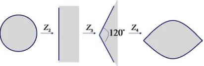
[image:11.595.315.521.130.197.2]The first example is a family of shapes for which the conformal mappings − and + can be solved analytically: these are the lens or eye shaped regions bounded by two circular arcs meeting at two corners. Figure5shows how the conformal map to the interior one such shape can be constructed. To get any other eye shaped region, one need only change the power in the third step and change the M¨obius map used in the final step. If the angle of the eye at its corners isαπ, then one uses z3=zα2. The same method gives us the
Figure 5. Example: The construction of−– the conformal map-ping of the interior of the unit disc onto the interior of the “eye” shape, presented in steps. The transformation z1=es+iθcarries the
real-plane (s,θ) to the complex-plane circle (most left), z2= 1−z1
1+z1
carries the circle to a half-plane (second left), z3=z23/2carries the half-plane to an “angled” half-plane (second right), and z4= 1−z3
1+z3
carries the angled half-plane to the eye shape (most right). Note that the same maps take the exterior of the unit circle to the exterior of the eye, except that the middle map must be replaced by z3=i z42/3. We can work out the fingerprint by going from z1to z2to z3which we equate to z3, then back to z2and to z1without going to z4at all. Using the fact that if z1 =eiθ, then z2 = −i tan(θ/2), we get the formula(θ)=2arctan(±|tan(θ/2)|1/2) where the sign is that of the tangent.
conformal to the exterior, except that as the exterior angle is (2−α)π, one uses z3 = z2−2 α. Applying this
construction to both the interior and the exterior, we can verify that the fingerprints which give eye shaped regions are all of the form:
β(θ)=2·arctan tan(θ/2)β,
where tanβ =sign(tan)|tan|β. (24) Here, ifαπ is the angle of the corner of the eye, then
β =α/(2−α). The fingerprint for one eye shape is shown in Fig.6.
It is striking that the formula for the fingerprint of eye-shaped regions is of the form f−1(β· f(θ)): in fact define f1 : (0, π) ←→ Rby f1(θ) = log(tan(θ/2))
and f2: (−π,0)←→Rby f2(θ)=log(−tan(θ/2)).
Then
β(θ)=
f1−1(β( f1(θ))) on (0, π) f2−1(β( f2(θ))) on (−π,0)
θifθ=0 orπ This formula makes apparent the identity:
β1β2=β1◦β2.
In this situation, the set of diffeomorphisms{β}is called a one parameter subgroup.
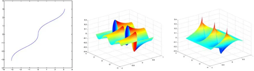
Figure 6. On the left, the fingerprint of the eye shape as given by Eq.24; in the middle and right, the functions k(s,θ) and h(s,θ) used in Sec.3.2.2to construct the shape from its fingerprint.
form is more general. To put theβ’s in this form, it’s convenient to decompose the circle into four intervals between the four fixed points {0, π/2, π, 3π/2} of
β. Then define g(θ) = log(|log(|tan(θ/2)|)|) at all
non-fixed points. Then:
β(θ)
=
g−1(log(β)+g(θ)), ifθ∈((k−1)π/2,kπ/2), some k
θifθ=kπ/2, some k.
The recipe generalizes like this: take any decomposi-tion of the circle into a set of intervals{Ik=(θk,θk+1)}.
On each interval, take a bijective map fk : Ik←→R.
Then define:
α(θ)=
fk−1(α+ fk(θ)), ifθ ∈Ik,
θ, ifθ=θk, some k.
Forαinfinitesimal, this diffeomorphism is given by the vector field:
v(θ)
=∂α∂ fk−1(α+fk(θ)) α=0= f
−1 k
( fk(θ))=
1
fk(θ)
.
In this way, every vector fieldvdefines a one-parameter subgroup, as is well known from the theory of Lie groups.
Here’s an elegant example of this: start with the Fourier basis for vector fields –vn(θ)=sin(nθ),n ≥
2. The zeros of these vector fields are the 2n points
{πk/n,0 ≤ k < 2n}: these will be the fixed points of the corresponding one-parameter subgroups. By integrating, we solve for fkand it comes out:
fk(θ)=
1
nlog
|tann 2θ|
.
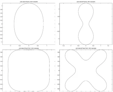
Welding, one finds wonderful n-petalled ‘flowers’ coming out as the corresponding shapes. As you move out on the one-parameter subgroup, increasingα, the petals start as small ripples, then extend and form al-ternating large circular evaginations and invaginations. This is shown in Fig.7.
Another simple example is the square (see Fig. 8). As mentioned above, the interior and exterior conformal maps are given by simple Schwarz-Christoffel expres-sions7, namely:
−(z)=
z
0 dζ
1−ζ4
+(z)=z+
z
∞
ζ4−1
ζ2 −1
dζ
From the eye and square examples (Figs. 6 and 8), the derivative of the conformal map on the interior goes to∞(shown by the spreading out of the internal ra-dial lines at the corners) while the derivative of the conformal map on the exterior goes to 0 (shown by the bunching up of the external radial lines). This is seen explicitly by noting that the derivative of the S-C formula is just its integrand and this is 0 (resp. ∞) at convex (resp. concave) corners. Thus the derivative of the fingerprint is ∞ at convex corners, 0 at con-cave corners. If the shape has high positive curvature at some point but not infinite as in a convex corner, we will find that the fingerprint has large derivative at the corresponding point; while points with large negative curvature, not −∞ as in a concave corner, the fingerprint has very small derivative at the corre-sponding point.
Figure 7. The shapes obtained by welding with (2/n)arctan(αtan(nθ/2)) for (n,α) equal to (2, 2) (top left), (2, 50) (top right), (4, 2) (bottom left) and (4, 50) (bottom right).
‘cigar-shaped’ blobs. One might have expected that these come from the one-parameter subgroup given by the vector field sin(2θ), but, as we saw, these shapes develop concavities. This is because they are symmet-rical with respect to inversion z →1/z. Although the exact fingerprint for specific large eccentricity ellipses or long blobs is hard to compute exactly, the follow-ing argument gives ffollow-ingerprints for one family of long blobs, as one verifies by welding. To construct this, we use 2 simple conformal maps which don’t quite match up and then we force them to match up! The exterior of a circle can be mapped to the whole plane minus the slit [−r+r] by the conformal map w=(r/2)(u+1/u). In
this map, the exterior of a circle|u| ≥λ, forλslightly greater than 1, is carried to the exterior of an ellipse sur-rounding the slit, with width r(λ+1/λ)≈2r and small height r(λ−1/λ). Unfortunately, the conformal map to the interior of the ellipse is not given by elementary functions. But one can map the interior of the circle to the strip|imag(w)|< π by the map w=2 log ((1+
z)/(1−z)), and this maps the interior of the circle|z| ≤
µ, forµslightly less than 1, to the interior of a cigar-shaped region inside this strip. This blob has height slightly less than 2π and width 4 log ((1+µ)/(1−
µ)). Both maps are illustrated in Fig.9.
The images of these circles roughly match up if we require that 2π = r(λ − 1/λ) and 4 log (((1 +
µ)/(1−µ))=r(λ+1/λ). We make an approximate fingerprint by mapping a point on the circle|z| =µto that point on the circle|u| =λfor which the real parts of the corresponding z-values are equal. This means: Re
r
2 λe
iθ1+λ−1e−iθ1=Re
2 log
1+µeiθ2
1−µeiθ2
.
or
r
2(λ+λ
−1) cosθ 1=log
1+µe
iθ2
1−µeiθ2 2
=log
1+νcosθ2
1−νcosθ2
, ν= 2µ
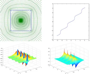
Figure 8. On the top left, internal and external conformal parametrization of the square. Top right, the fingerprint of the square; in the bottom, the functions k(s,θ) (left) and h(s,θ) (right) used in Sec.3.2.2to construct the shape from its fingerprint.
Figure 9. The construction of an explicit formula for the fingerprint of a long blob: on the left, (i) the red curve is an ellipse and its exterior is uniformized by w=(r/2)(u+1/u), (ii) the interior of the blue curve is uniformized by the map w=2 log ((1+z)/(1−z)) applied to a circle
with radius slightly less than 1. The fingerprint on the right is made by matching points on these with the same real part and the yellow curve on the left is the result of welding with this fingerprint.
Simplifying, we get the formula for the fingerprints of long blobs,blob1as:
θ1=arccos
log
1+νcosθ2
1−νcosθ2
log
1+ν 1−ν
In this form, the fingerprint has high derivatives at 2 points, corresponding to the 2 ends of the blob and the interior conformal map takes 0 to the center of the blob. The same shape, however, is defined byblob1◦A for
[image:14.595.96.503.482.590.2]one end of the blob. Then the fingerprint will only have high derivatives at one point. With some experimenta-tion, one finds a simple form for such a fingerprint:
blob2(θ)=
2arctan
C1
log(1+a tan2(θ/2)),ifθ∈[−θ 0, θ0]
2arctan (tan(θ/2)+C2sign(θ)), ifθ∈(−π, π)−[−θ0, θ0]
where C1, C2are chosen to make the above continuous
with continuous derivatives8.
We can use the formula for elongated blobs to illus-trate the power of the group law in Diff(S1). Suppose
1 and2 are the fingerprints of 2 shapes. We can
combine them in various ways using the fingerprints
1◦A◦2, for various M¨obius maps A. As A varies,
the mode of combination varies. We take1=blob2
to be the fingerprint of a suitable blob and2=boom
to be the fingerpint of a ‘boomerang’ shape computed by Schwarz-Chistoffel. To combine them, we will first pick the constants a andθ0in the blob fingerprint so that
blob1is close to the identity over much of its domain,
and has very large derivative at one point. Then we combine them with a rotation R inserted. In fact, to put the boomerang back in a fixed orientation, we show in Fig.10the shapes defined by R−1◦blob1◦R◦boom.
The effect will be to create a new shape in which a blob is glued to the boomerang at a point depending on where this derivative is large.
Finally, we look at two more complex shapes. The first is a silhouette of a cat. For this we apply the Schwarz-Christoffel package in order to obtain(θ). Hence (θ), (θ) and −1(θ) involved in Eq. 13 are computed numerically. We reconstrcut the shape using the first welding method. The result is shown in Fig. 11. Note again the close similarity of the com-puted(right) to the original shape (left). Recall from Eq.14the way k and h (Fig.11, bottom row) describe
. In our current straightforward implementation we are limited in the size of the (s,θ)-grid we can solve for. This results in the minor distortions in k, h and the resulting.
The final example is the silhouette of the upper body of a person (see Fig.12).
5. The WP Riemannian Metric onS
5.1. The WP Norm on the Lie Algebra of Diff(S1)
The Lie algebra of the group Diff(S1) is given by the
vector space vec(S1) of smooth vector fields on the
circle:v(θ)∂/∂ θwherev(θ+2π)=v(θ). In general, the adjoint action of a group element g∈G is the linear
map from Lie(G) to itself induced by the conjugation
map h→g−1◦h◦g from G to itself. Explicitly, this
mapsv∈vec(S1) to (v◦g)/g, i.e. adg(v)=(v◦g)/g.
We can expand such av in a Fourier seriesv(θ)=
∞
n=−∞anei nθ(where an=a−n). The Weil-Petersson
norm on vec(S1) is defined by:
||v||2 W P =
∞
n=2
(n3−n)|an|2.
The null space of this norm is given by those vector fields whose only Fourier coefficients are a−1, a0and a1, i.e. the vector fields (a+bcos(θ)+csin(θ))∂/∂θ, which are exactly those tangent to the M¨obius subgroup
PSL2(R), i.e. in its Lie algebra psl2(R).
The motivation for this particular definition is the fact that, for allφ∈PSL2(R) andv∈vec(S1), one can verify that
||adφ(v)||W P = ||v||W P. 5.2. Extending the Metric to Diff(S1)/PSL
2(R)
Riemannian metrics on coset spaces G/H which are invariant by all left multiplication maps Lg : G/H→ G/H, g∈G are given by norms ||v|| on the Lie algebra of G which are zero on the Lie subalgebra of H and which satisfy ||adh(v)||=||v|| for all h∈H. Here the
norm on the tangent space TgH,G/H to G/H at any gH
is gotten from the norm on the Lie algebra via the isomorphism
DLg : Lie(G)/Lie(H )=Te H,G/H→Tg H
given by the derivative of Lg at the identity e of G.
In particular, this applies to Diff(S1) and PSL2(R).
Because Diff(S1)/PSL2(R) ∼= S, we have now con-structed a homogeneous Riemannian metric onSalso. Next let’s translate this into concrete terms. Take any path(t,θ) in Diff(S1), where t ∈ [0,t
0] ⊂ R
and(t, θ +2π) = (t, θ)+2π. The tangent vec-tors to this path are given by ∂∂(tt,θ) = t(t, θ) or,
Figure 10. Top-left: the boomerang shape, middle-left: its fingerprint, middle-right: the fingerprint of the blob, and bottom-left: the fingerprint of a composition. Note the very large derivative on the boomerang fingerprint for two ends, and the very small derivative for the concave corner. The blob fingerprint has one point of high derivative corresponding to the far end, the origin being placed at the near end. A rotation is used in the composition, and the small circles mark corresponding points in the graphs of the 3 diffeo-morphisms. On the top-right and bottom-right: shapes defined by compositions of the fingerprints with various rotations and constants. The composite shapes can be interpreted as the boomerang plus a blob at some point of its boundary—short on the top-right, much longer than the boomerang itself on the bottom-right. In the composite shapes on the left, the blob’s constants are a=e20, on the right
a=e50, whileθ0=.05 radians in both cases. For each set of constants, rotations through kπ/10 radians have been put in the middle so that the protrusions are placed on the boomerang at different points of its boundary.
t(t, θ)/θ(t, θ).We expand the tangent vector at
ev-ery t ≥0 by its Fourier series inθ:
t(t, θ)/θ(t, θ)= ∞
n=−∞
an(t)ei nθ, (25)
where a−n(t) =an(t) because the vector field is real.
Its Weil-Petersson norm is then given by
t(t, θ)/θ(t, θ)WP =. ∞
n=2
Figure 11. Top: the conformal mappings−and+carrying a homogenous radial grid (left, drawn schematically) onto the interior and exterior of the cat silhouette; middle line: the fingerprint of the cat and the cat, as reconstructed by welding following the first method; bottom: the harmonic functions k (left) and h (right) used for reconstruction.
and the length of the path is by definition:
t0 0
∞
n=2|an(t)|2(n3−n)dt.
It is a wonderful fact that all sectional curvatures of the Weil-Petersson norm are non-positive (Bowick and Lahiri,1988). Because of this, it is to be expected that there is a unique geodesic joining any two shapes9 1, 2 ∈ S. Because minimizing energy and length
are equivalent, these geodesics are the solutions of the following minimization problem
Min(t,θ),t0 t0
t=0 ∞
n=2
|an(t)|2(n3−n)dt, (27)
where (0,θ) and(t0,θ) are the diffeomorphisms
Figure 12. A truncated human figure. On the left, the conformal parametrization of the interior and exterior; in the middle, the fingerprints; on the right, the reconstruction using the first method.
6. Calculating the Geodesics
We solve for the geodesics{(t,θ)}t∈[0,1], where(t,
θ) ∈Diff(S1)∀t ∈[0, 1], parameterized by ‘time’ t
between the two given end-point shapes0=. (0, θ)
and1 =. (1, θ). The length of the geodesic between
each two given end-point shapes is obtained by mini-mizing the Weil-Petersson norm
1
0
t(t, θ)/θ(t, θ)WPdt, (28)
where 0 and 1 are the diffeomorphisms
(finger-prints) corresponding to the two given end-point shapes (see Sec.5.2).
Minimizing the norm in Eq.28is equivalent to min-imizing the energy
E(0, 1)=.
1
0 ∞
n=2
|an(t)|2(n3−n)dt, (29)
(cf. Sec.5.2), where
t(t, θ)/θ(t, θ)= ∞
n=−∞
an(t)ei nθ (30)
We discretize t ∈ [0, 1] into M homogenously spaced points tu = Mu, u = 0,1,2, . . . ,M, and
we discretize θ ∈ [−π, π] into N homogenously spaced pointsθk = −π+2Nπk, k =0,2, . . . ,N −1.
We will always choose N = 2n, and M = 2m for
suitable n, m. We discretize the geodesics using a
(k, u)-grid into {(tu, θk)}k,u, where k = 0, 2, . . . , N−1, and u=0, 2, . . . , M. Both 0 = {. (t0, θk)}k
and 1 = {. (tM, θk)}k are fixed as the end-point
diffeomorphisms. In addition it is convenient for com-puting the energy (Eq.29) to discretize the parameter
t in the integral using also a shifted u-grid, namely an s-grid for which ts = 2M1 + Ms, s =1,2, . . . ,M. We
denote ts− =. ts− 2M1 and ts+ =. ts +2M1 , so that the
grids s−and s+coincide with points of the u grid. We can therefore discretize
θ(ts, θk)∼=
1 2
(ts+, θk+1)−(ts+, θk−1)
4π/N
+(ts−, θk+1)−(ts−, θk−1)
4π/N
,(31) and
t(ts, θ)∼=
(ts+, θ)−(ts−, θ)
1/M , (32)
thus obtaining the following discretization:
t(ts, θk)
θ(ts, θk) ∼ =
M N
8π
(ts+, θk)−(ts−, θk)
(ts+, θk+1)+(ts−, θk+1)−(ts+, θk−1)−(ts−, θk−1)
(33) To compute the geodesics {(tu,θk)}k,u, we will
therefore minimize the discretized version of Eq.29
E(0,1)=. M
s=1 N−2
n=2
Figure 13. A geodesic: rotating the ellipse byπ/3, clockwise.
Figure 14. A geodesic from the ellipse with eccentricity 2 to a square.
where∀s=1,2, . . . , M and k=0, 1, . . . , N−1 we have the discrete Fourier transform
t(ts, θk)
θ(ts, θk) = 1
N N/2
n=0
an(ts)e2πi nk/N, aN−n(ts)=an(ts).
(35) (cf. Eq.30, but now with maximum frequency N/2).
We denoteE0,1=. E (0,1),k,u =. (tu, θk), and
s±,u=. (ts±, θk).
6.1. Direct Computation of the Energy Gradient
∂E0,1/∂k,u
Figure 15. A geodesic from a square with a left bulge to the same square with a right bulge.
Figure 16. A geodesic from a Mickey-Mouse-like shape to a Donald-Duck-like shape.
formula for directly computing its gradient ∂E0,1/
∂k,u. To obtain this we define
wk=. ˜k3−˜k, where ˜k=min(k,N−k). (36)
We then define {w1}1=0N−1 to be the discrete Fourier
transform of{wl}lN=0−1. That is
wl = N−1
k=0
[image:20.595.148.447.387.612.2]