Predicting interval and screen detected breast cancers from mammographic density defined by different brightness thresholds

R E S E A R C H A R T I C L E

Open Access

Predicting interval and screen-detected

breast cancers from mammographic

density defined by different brightness

thresholds

Tuong L. Nguyen

, Ye K. Aung

, Shuai Li

, Nhut Ho Trinh

, Christopher F. Evans

, Laura Baglietto

,

Kavitha Krishnan

, Gillian S. Dite

, Jennifer Stone

, Dallas R. English

, Yun-Mi Song

, Joohon Sung

,

Mark A. Jenkins

, Melissa C. Southey

, Graham G. Giles

and John L. Hopper

Abstract

Background:Case–control studies show that mammographic density is a better risk factor when defined at higher than conventional pixel-brightness thresholds. We asked if this applied to interval and/or screen-detected cancers. Method:We conducted a nested case–control study within the prospective Melbourne Collaborative Cohort Study including 168 women with interval and 422 with screen-detected breast cancers, and 498 and 1197 matched controls, respectively. We measured absolute and percent mammographic density using the Cumulus software at the conventional threshold (Cumulus) and two increasingly higher thresholds (AltocumulusandCirrocumulus, respectively). Measures were transformed and adjusted for age and body mass index (BMI). Using conditional logistic regression and adjusting for BMI by age at mammogram, we estimated risk discrimination by the odds ratio per adjusted standard deviation (OPERA), calculated the area under the receiver operating characteristic curve (AUC) and compared nested models using the likelihood ratio criterion and models with the same number of parameters using the difference in Bayesian information criterion (ΔBIC).

Results:For interval cancer, there was very strong evidence that the association was best predicted byCumulusas a percentage (OPERA = 2.33 (95% confidence interval (CI) 1.85–2.92); allΔBIC > 14), and the association with BMI was independent of age at mammogram. After adjusting for percentCumulus, no other measure was associated with risk (all

P> 0.1). For screen-detected cancer, however, the associations were strongest for the absolute and percentCirrocumulus measures (allΔBIC > 6), and after adjusting forCirrocumulus, no other measure was associated with risk (allP> 0.07). Conclusion:The amount of brighter areas is the best mammogram-based measure of screen-detected breast cancer risk, while the percentage of the breast covered by white or bright areas is the best mammogram-based measure of interval breast cancer risk, irrespective of BMI. Therefore, there are different features of mammographic images that give clinically important information about different outcomes.

Keywords:Breast cancer, Masking effect, Interval cancer, Screen-detected, Nested case–control cohort study, Australian women, Mammography, Mammographic density

* Correspondence:[email protected]

1_{Centre for Epidemiology and Biostatistics, The University of Melbourne,}

Level 3/207 Bouverie Street, Carlton, VIC 3053, Australia Full list of author information is available at the end of the article

Background

Mammographic images can be used for more than identi-fying existing breast tumours–they contain information that predicts both (1) the risk of future breast cancers and (2) the likelihood of existing tumours being missed due to masking [1]. This has important implications for future breast cancer control because of the widespread use of mammography screening. Women could be triaged according to their risk of disease and/or masking so as to implement tailored screening, and deal with the ongoing need to improve cost-effectiveness, minimise harm [2,3], and help address the issue of“dense breasts”[4].

Conventionally, mammographic density has been defined as the white or bright areas on a mammogram and, after adjusting for age and body mass index (BMI), has been found to be a risk factor for both interval and screen-de-tected breast cancers [1,5,6]. Screen-detected breast can-cers are cancan-cers detected via a screening programme and interval breast cancers are those detected within 2 years of a mammographic screen that did not detect any breast can-cer. Interval cancers are in general more aggressive [6–11], so it is important to understand if the relationship between mammographic density measures and breast cancer risk differs by mode of detection [12].

We previously found, from case-control studies of both Australian [13] and Korean [14, 15] women, that by defining mammographic density at higher than con-ventional pixel-brightness thresholds we obtained better discrimination between women with and without breast cancer. This applied for both film and digital mammo-grams. It is not known, however, if this observation differs according to mode of detection. In this study, we have used a prospective cohort and asked if, and how well, the conventional and our new mammographic density mea-sures apply to interval and screen-detected breast cancers.

Materials and methods Subjects

We used the prospective Melbourne Collaborative Cohort Study of Australian-born, Italian-born, and Greek-born male and female adult residents of Melbourne [16,17]. We conducted a nested case–control study in which cases were women who had been diagnosed with a first diagnosis of ductal carcinoma in situ or invasive adenocarcinoma of the breast (C50.0-C50.9) since the baseline survey. Cases were ascertained by record linkage to the population-complete Victorian Cancer Registry and to the Australian Cancer Database. Controls had been matched for year at birth, year of baseline interview, and country of origin [12, 18]. Controls were selected randomly from those who had not been diagnosed with breast cancer at the age of diagnosis of the case. Participants completed interviewer-adminis-tered questionnaires that captured standard risk factors for breast cancer, including reproductive history. Height and

weight were measured directly according to standard pro-tocols and BMI was calculated from these. We studied only those female cohort members who had attended BreastScreen Victoria (the state-organised, free, 2-yearly, mammographic screening service for women aged 50 to 69 years) at least once for a mammogram, and did not have a diagnosis of breast cancer when they completed their baseline questionnaire. Family history of breast cancer in any blood relative, as collected by BreastScreen Victoria, was available for all participants.

Breast cancers were identified by BreastScreen Victoria, or by linkage with the Victorian Cancer Registry. Breast cancers diagnosed outside the screening service before the next scheduled scan (2 years) after a negative scan were classified as interval cancers, and those subsequently iden-tified by BreastScreen Victoria at a scheduled scan were classified as screen-detected. Consequently, the study in-cluded two subgroups: 422 women with screen-detected breast cancers (357 of which were invasive) with 1197 matched controls and 168 women with interval breast cancers (148 of which were invasive) with 498 matched controls. For this study, we selected the mammogram closest to baseline (average 2 years difference [18]), and this was on average 5 or 6 years prior to diagnosis for interval and screen-detected cases, respectively; see Table1 in a previous publication [12]. The study was approved by the human research ethics committees of the University of Melbourne and the Cancer Council Victoria.

Measurement of mammographic density

measurer considers to be the dense tissue and the programme calculates the absolute dense area. This is done separately for the three density measures, each according to their different definitions of density, given above.

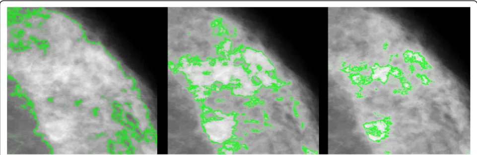
Figure 1 shows, for a particular section of the same mammogram, how the dense areas (outlined in green) vary depending on the definition of mammographic density. The left panel shows the region classified asCumulus, and the centre panel shows that within this region there are brighter areas that are classified asAltocumulus. Similarly, within the latter regions, the right panel shows that there are even brighter areas that are classified asCirrocumulus.

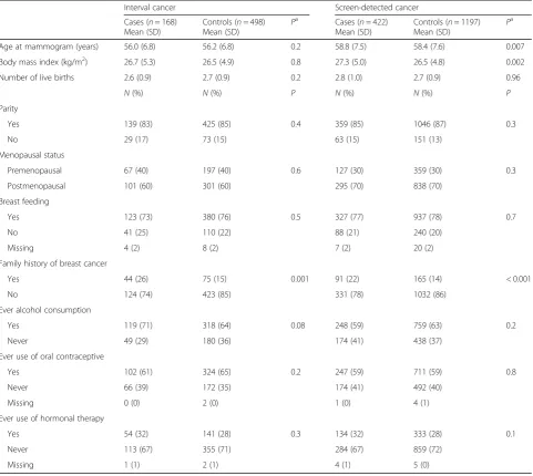
For each definition of mammographic density, we used the average over all measurers of their transformed, age-adjusted, BMI-adjusted and standardised measures so as to maximise the accuracy; see “Statistical methods”. Correl-ation between the resulting dense area and percent density measures was 0.87, 0.92, and 0.96 for Cumulus, Alto-cumulus, and Cirrocumulus, respectively. Correlation between the Cumulus and Altocumulus measures was 0.86 for dense area and 0.88 for percent density. The corresponding correlation between theCumulusand Cirro-cumulusmeasures was 0.82 and 0.82, respectively, and the corresponding correlation between the Altocumulus and Cirrocumulusmeasures was 0.82 and 0.82, respectively. Table 1Characteristics (mean (SD), or number (percentage)) of patients (cases) and controls, by mode of detection (screen-detected or interval breast cancer)

Interval cancer Screen-detected cancer

Cases (n= 168) Mean (SD)

Controls (n= 498) Mean (SD)

Pa _{Cases (n= 422)} Mean (SD)

Controls (n= 1197) Mean (SD)

Pa

Age at mammogram (years) 56.0 (6.8) 56.2 (6.8) 0.2 58.8 (7.5) 58.4 (7.6) 0.007

Body mass index (kg/m2_{) 26.7 (5.3) 26.5 (4.9) 0.8 27.3 (5.0) 26.5 (4.8) 0.002}

Number of live births 2.6 (0.9) 2.7 (0.9) 0.2 2.8 (1.0) 2.7 (0.9) 0.96

N(%) N(%) P N(%) N(%) P

Parity

Yes 139 (83) 425 (85) 0.4 359 (85) 1046 (87) 0.3

No 29 (17) 73 (15) 63 (15) 151 (13)

Menopausal status

Premenopausal 67 (40) 197 (40) 0.6 127 (30) 359 (30) 0.3

Postmenopausal 101 (60) 301 (60) 295 (70) 838 (70)

Breast feeding

Yes 123 (73) 380 (76) 0.5 327 (77) 937 (78) 0.7

No 41 (25) 110 (22) 88 (21) 240 (20)

Missing 4 (2) 8 (2) 7 (2) 20 (2)

Family history of breast cancer

Yes 44 (26) 75 (15) 0.001 91 (22) 165 (14) < 0.001

No 124 (74) 423 (85) 331 (78) 1032 (86)

Ever alcohol consumption

Yes 119 (71) 318 (64) 0.08 248 (59) 759 (63) 0.2

Never 49 (29) 180 (36) 174 (41) 438 (37)

Ever use of oral contraceptive

Yes 102 (61) 324 (65) 0.2 247 (59) 711 (59) 0.8

Never 66 (39) 172 (35) 174 (41) 492 (40)

Missing 0 (0) 2 (0) 1 (0) 4 (1)

Ever use of hormonal therapy

Yes 54 (32) 141 (28) 0.3 134 (32) 333 (28) 0.1

Never 113 (67) 355 (71) 284 (67) 859 (72)

Missing 1 (1) 2 (1) 4 (1) 5 (0)

SDstandard deviation

a_P

Repeatability was assessed by performing the measure-ments in 18 sets of 100 mammograms with the same ratio of cases and controls and including 10% repeat samples randomly in each set, to estimate intra-class correlation within the set. In the 5th, 10th, and 15th sets, there was also a 10% repeat sample from the first batch to estimate intra-class correlation between the sets. Consequently, 110 images were included in all batches except for batches 5, 10, and 15, which had 120 images.

For dense area, the within-set repeatability was 0.95 (95% confidence interval 0.94–0.96), 0.96 (0.94–0.97) and 0.94 (0.90–0.94) for the average ofCumulus, Altocumulus, and Cirrocumulus, respectively. For dense area, the between-set repeatability was 0.95 (0.93–0.97), 0.95 (0.94–0.96) and 0.94 (0.92–0.94) for the average ofCumulus, Altocumulus, and Cirrocumulus, respectively. Similar repeatability was obtained for the percent density measures. The average of the inter-observer correlation was 0.90, 0.92, and 0.87 for Cumulus,Altocumulus, andCirrocumulus, respectively.

Statistical methods

Unconditional logistic regression was used to test for differences between independent sub-groups of cases defined by mode of detection. Conditional logistic regres-sion was used to test for differences between cases and matched controls, and to estimate odds ratios between the mammographic density measures and breast cancer risk, separately for screen-detected breast cancer and interval breast cancer, adjusting for covariates. Given the change in direction of association between BMI and breast cancer risk with increasing age, we included an interaction term to test if the odds ratio for BMI in relation to breast cancer risk depended on age at mammogram. Each mammographic density measure was transformed using a Box–Cox power transformation to have an approxi-mately normal distribution by using maximum likelihood to estimate the parameterλsuch that (Yλ–1)/λis closest

to a normal distribution [20]. For each fitted model, the mean of the transformed measures for the controls was adjusted for age and BMI to derive the residuals, from which their standard deviation was calculated.

As in our previous publications [13–15], we used this ad-justed standard deviation and conditional logistic regression to estimate the odds ratio per adjusted standard deviation (OPERA, [21]). OPERA is a measure of the ability of a risk factor (appropriately adjusted for the covariates taken into account by design and analysis) to discriminate between cases and controls. When we fitted two standardised density measures, X1and X2, into the same model, we

presented the risk estimates in terms of their standard deviation (SD) after adjusting also for the other measure; see (14). We did this by multiplying the log(OR) estimate from fitting Xj by SD = [(1 – r2)]0.5, where r is the correlation

betweenX1andX2, and then exponentiated it to obtain

the appropriate OPERA. The inter-quartile risk ratio (IQQR) corresponding to a given OPERA is approximately OPERA2.5. We also used the area under the receiver oper-ator curve (AUC) to measure the discriminoper-atory ability of measures. All statistical analyses were conducted using the software Stata [22], and following convention,P< 0.05 was considered to be statistically significant.

Parameter estimates were derived under asymptotic maximum likelihood theory. We compared the fits of nested models using the likelihood ratio criteria; under the null hypothesis, twice the absolute difference in the (maximum) log likelihood (ΔLL) has an approximately χ2

distribution with degrees of freedom equal to the difference in number of parameters. The fits of models were also compared based on the differences in the Bayesian information criterion (ΔBIC), which for models with the same number of parameters is 2ΔLL. IfΔBIC is the BIC of model A minus the BIC score of model B, then exp (-ΔBIC) is approximately equal to the posterior odds in favor of model A; for example, ΔBIC =−6 or−14

means that model A is roughly 400 or 1,000,000 times, respectively, more likely to be the model that generated the data than model B. The strengths of evidence against the model with the poorest fit are conventionally inter-preted as non-existent if < 2, positive if 2–6, strong if 6– 10, and very strong if≥10 [23].

Results

Table 1 shows that women with interval breast cancer did not differ from their matched controls in any base-line characteristic, including BMI, except for family history (P≤0.001). Screen-detected cases differed from their matched controls in family history (P< 0.001) and BMI (P= 0.003).

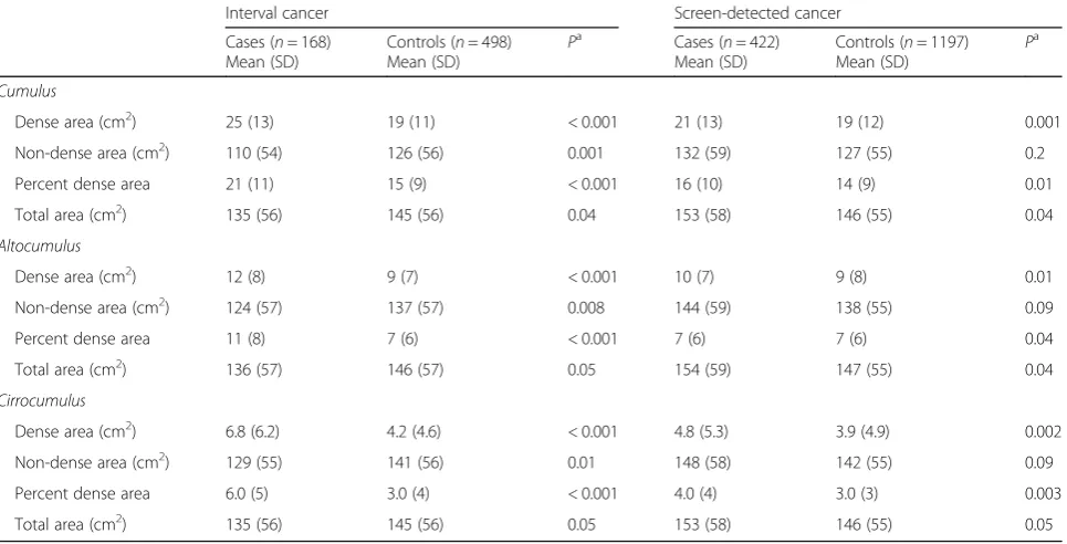
Table2shows that the unadjustedCumulus,Altocumulus andCirrocumulus measures of dense area were all greater for cases than for controls, for both interval and screen-de-tected breast cancer (allP< 0.01). Percent dense area mea-sured by Cumulus, Altocumulus and Cirrocumulus was greater for cases with interval breast cancers compared with (1) their controls (all P< 0.001), and (2) cases with screen-detected breast cancers (allP< 0.001).

For interval cancer, the association with BMI did not depend on age at mammogram (P> 0.8). There was no as-sociation with BMI overall (see Table1). Screen-detected cancer was associated with BMI and the association became stronger with age at mammogram (P< 0.02).

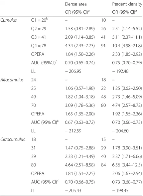
Table 3 shows that, for interval breast cancer, after adjusting for age and BMI all of the dense area measures

were associated with breast cancer risk (all P< 0.001). The log (OPERA) was 0.61, 0.50 and 0.61 for Cumulus, AltocumulusandCirrocumulus, respectively (allP< 0.001), There was very strong evidence that the Cumulus and Cirrocumulus measures gave a better fit than the Alto-cumulusmeasure (bothΔBIC≥10).

For percent density measures, there was very strong evidence that the OPERA estimates were all higher than for their corresponding absolute density measure (all ΔBIC≥10), especially forCumulus where log (OPERA) was 0.85 compared with 0.65 and 0.72 for Altocumulus andCirrocumulus, respectively (allP< 0.001). and that the Cumulusmeasure gave a better fit than theCirrocumulus and Altocumulus measures (both ΔBIC ≥10). The risk gradient forCirrocumulus was 30% and 17% higher than for the other two measures, respectively. Furthermore, there was very strong evidence that theCumuluspercent density measure gave a better fit than the Cumulus absolute density measure (ΔBIC = 28), with an estimated risk gradient 39% higher. Univariately, therefore, the Cumulus percent density measure gave a better fit for interval cancers, with an estimated risk gradient equivalent to an IQQR ~ 8-fold (95% CI 5–15).

Table 4 shows that, for screen-detected breast cancer, all the dense area measures were associated with risk, after adjusting for age and BMI as an interaction due to the aforementioned findings (paragraph 3, “Results”) (P< 0.001). The log OPERA was 0.22, 0.22 and 0.28 for the transformed, normalized and standardized Cumulus,

Table 2Mammographic density measurements for cases and controls, by mode of detection (screen-detected or interval cancer)

Interval cancer Screen-detected cancer

Cases (n= 168) Mean (SD)

Controls (n= 498)

Mean (SD) P

a

Cases (n= 422) Mean (SD)

Controls (n= 1197)

Mean (SD) P

a

Cumulus

Dense area (cm2_{) 25 (13) 19 (11) < 0.001 21 (13) 19 (12) 0.001}

Non-dense area (cm2_{) 110 (54) 126 (56) 0.001 132 (59) 127 (55) 0.2}

Percent dense area 21 (11) 15 (9) < 0.001 16 (10) 14 (9) 0.01

Total area (cm2_{) 135 (56) 145 (56) 0.04 153 (58) 146 (55) 0.04}

Altocumulus

Dense area (cm2_{) 12 (8) 9 (7) < 0.001 10 (7) 9 (8) 0.01}

Non-dense area (cm2_{) 124 (57) 137 (57) 0.008 144 (59) 138 (55) 0.09}

Percent dense area 11 (8) 7 (6) < 0.001 7 (6) 7 (6) 0.04

Total area (cm2_{) 136 (57) 146 (57) 0.05 154 (59) 147 (55) 0.04}

Cirrocumulus

Dense area (cm2) 6.8 (6.2) 4.2 (4.6) < 0.001 4.8 (5.3) 3.9 (4.9) 0.002

Non-dense area (cm2) 129 (55) 141 (56) 0.01 148 (58) 142 (55) 0.09

Percent dense area 6.0 (5) 3.0 (4) < 0.001 4.0 (4) 3.0 (3) 0.003

Total area (cm2) 135 (56) 145 (56) 0.05 153 (58) 146 (55) 0.05

SDstandard deviation

a

AltocumulusandCirrocumulusmeasures, respectively (allP < 0.001). There was strong evidence that theCirrocumulus measure gave a better fit than theCumulusand Altocumu-lusmeasures (ΔBIC = 8). On the log odds scale, the risk gra-dient forCirrocumuluswas 24% higher than for the other two measures. Results were similar for the percent density measures adjusted for age and BMI.

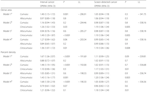
Table5shows that, for interval breast cancer, once we adjusted for Cumulus as a percentage, using the likeli-hood ratio test and comparing with the log likelilikeli-hood of 192.48 from Table 3showed there was no evidence that adding one or both of the other measures improved the fit (allP> 0.1). For example, when fitted together the OPERAs for the Cumulus attenuated but remained significant (P< 0.001) whereas the Altocumulus and Cirrocumulus

estimates were reduced substantially and were no longer significant (allP> 0.07). In particular, adding the Cirro-cumulus measure made no improvement to the fit (ΔLL = 0.7).

On the other hand, Table 5 shows that for screen-de-tected breast cancer it wasCirrocumulusthat was a sig-nificant predictor (all P< 0.01) irrespective of which other measure(s) were in the model, and for both dense area and percent dense area measures. After adjusting for Cirrocumulus, using the likelihood ratio test and compar-ing with the log likelihoods of−538.21 and−536.75 from Table4, respectively, showed no evidence that adding the other measures improved the fit (allΔLL < 0.1). In particu-lar, theCumulusmeasures no longer predicted risk in all multivariable models; their OPERAs were close to 1.0 and Table 3For interval breast cancer, marginal odds ratios, area

under the receiver operating characteristic curve (AUC) and log likelihood (LL) forCumulus,AltocumulusandCirrocumulus measures of dense area and percent density, adjusted for age and body mass index (BMI)

Dense area Percent density

OR (95% CI)a OR (95% CI)a

Cumulus Q1 = 20b _{– 10 –}

Q2 = 29 1.53 (0.81–2.89) 26 2.51 (1.14–5.52)

Q3 = 41 2.09 (1.14–3.85) 41 5.11 (2.37–11.1)

Q4 = 78 4.34 (2.43–7.73) 91 10.4 (4.98–21.8)

OPERA 1.84 (1.50–2.26) 2.33 (1.85–2.92)

AUC (95%CI)c _{0.70 (0.65–0.74) 0.75 (0.70–0.79)}

LL −206.95 −192.48

Altocumulus 24 – 18 –

25 1.06 (0.57–1.98) 22 1.25 (0.62–2.50)

49 1.82 (1.04–3.18) 48 2.73 (1.46–5.09)

70 3.09 (1.78–5.36) 80 4.74 (2.57–8.72)

OPERA 1.65 (1.35–2.00) 1.92 (1.55–2.36)

AUC (95% CI)c _{0.67 (0.63–0.72) 0.70 (0.66–0.75)}

LL −212.59 −204.60

Cirrocumulus 18 – 15 –

31 1.47 (0.75–2.88) 29 1.78 (0.90–3.51)

39 2.33 (1.21–4.49) 40 3.37 (1.71–6.66)

80 4.64 (2.51–8.58) 84 6.56 (3.44–12.5)

OPERA 1.84 (1.51–2.25) 2.06 (1.67–2.54)

AUC (95% CI)c _{0.70 (0.66–0.75) 0.73 (0.68–0.77)}

LL −205.43 −198.45

Odds ratios (OR) are shown by quartiles (number of cases shown in parentheses)

OPERAchange in OR per adjusted standard deviation,CIconfidence interval

a

Odds ratio per standard deviation adjusted for age and BMI

b

Quartiles (Q1–Q4) defined by distribution of the measure adjusted for age, BMI and number of livebirths

c

AUCs for mammographic measurements after adjusting for age and BMI

Table 4For screen-detected breast cancer, marginal odds ratios, area under the receiving operating characteristic curve (AUC) and log likelihood (LL) forCumulus,Altocumulusand

Cirrocumulusmeasures of dense area and percent density

adjusted for age and body mass index (BMI)

Dense area Percent density

OR (95% CI)a OR (95% CI)a

Cumulus Q1 = 88b _{– 81 –}

Q2 = 96 1.01 (0.72–1.41) 94 1.20 (0.85–1.69)

Q3 = 88 0.99 (0.70–1.39) 98 1.12 (0.80–1.59)

Q4 = 150 1.66 (1.22–2.27) 149 1.95 (1.41–2.70)

OPERA 1.25 (1.12–1.40) 1.30 (1.16–1.45)

AUC (95% CI)c _{0.63 (0.60–0.66) 0.64 (0.61–0.67)}

LL −542.27 −539.87

Altocumulus 81 – 85 –

97 1.19 (0.84–1.66) 85 1.00 (0.71–1.42)

98 1.28 (0.92–1.79) 114 1.31 (0.95–1.81)

146 1.86 (1.35–2.56) 138 1.72 (1.24–2.37)

OPERA 1.25 (1.12–1.40) 1.27 (1.14–1.43)

AUC (95% CI)c _{0.63 (0.60–0.66) 0.64 (0.60–0.67)}

LL −542.23 −541.29

Cirrocumulus 79 – 72 –

94 1.32 (0.93–1.87) 408 1.63 (1.15–2.32)

102 1.38 (0.98–1.94) 99 1.35 (0.95–1.92)

147 2.08 (1.50–2.87) 143 2.29 (1.63–3.22)

OPERA 1.32 (1.18–1.48) 1.35 (1.20–1.52)

AUC (95% CI)c _{0.64 (0.61–0.67) 0.64 (0.61–0.68)}

LL −538.21 −536.75

Odds ratios (OR) are shown by quartiles (number of cases shown in parentheses

OPERAchange in OR per adjusted standard deviation,CIconfidence interval

a

OR per standard deviation adjusted for age and BMI

b

Quartiles (Q1–Q4) defined by distribution of the measure adjusted for age, BMI and number of livebirths

c

not significant whether considered as percent or absolute dense area.

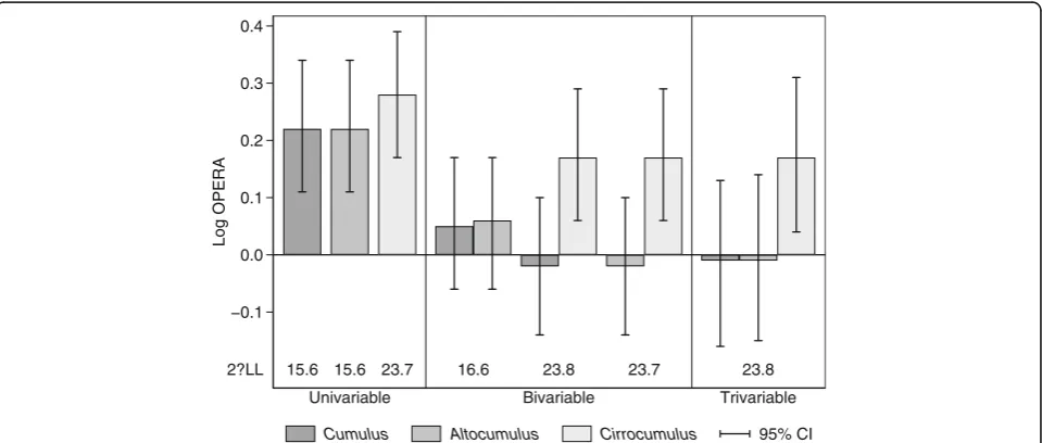
Figures2and3illustrate the relative stability of the risk measures by plotting the OPERAs and their confidence intervals as reported in Table3,4and5, on the log scale. For the percentage measures and interval cancers, the Cumulusmeasure dominates (see Fig.2), while for dense measures and interval cancers theCirrocumulusmeasure dominates (see Fig. 3). The patterns in estimates across the models are seen to be clearly different for the two outcomes.

Additional file 1: Tables S1 and S2 show the results of analyses when restricted to invasive cancers only. The aforementioned general patterns observed were maintained. Additional file 1: Table S3 shows that fitting different models to different modes of detection made a highly significant improvement in fit compared with fitting one model to the combined data - which assumes that estimates

are the same for both screendetected and interval cancers -for all models (allP< 0.005).

Discussion

We found that the risk predictors for breast cancer differ by mode of detection. First, there was very strong evidence that interval breast cancers are best predicted when mammographic density was defined conventionally as the white or bright areas, the more so when defined as a percentage. It was more than 20,000 times more likely to be the measure that generated the data than either of the other two measures. Addition of the other measures did not add information, and BMI did not appear to be a predictor of interval disease. On the other hand, we found very strong evidence that screen-detected breast cancers are best predicted by mammographic density when de-fined as the brighter areas on a mammogram, whether as an absolute or percentage measure. The Cirrocumulus Table 5For interval and screen detected breast cancer, multivariable odds ratios, area under the receiving operating characteristic curve (AUC), and log likelihood (LL) forCumulus,AltocumulusandCirrocumulusmeasures of dense area and percent density adjusted for age and body mass index (BMI)

Interval cancer P LL Screen-detected cancer P LL

OPERA (95% CI) OPERA (95% CI)

Dense area

Model 1a _{Cumulus 1.40 (1.15–1.72) 0.001 −206.91 1.05 (0.94–1.19) 0.3 −541.75}

Altocumulus 0.97 (0.80–1.18) 0.8 1.06 (0.94–1.19) 0.3

Model 2b _{Cumulus 1.16 (0.94–1.43) 0.2 −204.46 0.98 (0.87–1.10) 0.8 −538.16}

Cirrocumulus 1.26 (1.02–1.53) 0.03 1.19 (1.06–1.34) 0.005

Model 3c _{Altocumulus 0.94 (0.76–1.16) 0.6 −205.27 0.98 (0.87–1.10) 0.8 −538.18}

Cirrocumulus 1.49 (1.20–1.87) < 0.001 1.19 (1.06–1.34) 0.005

Model 4d _{Cumulus 1.27 (0.99–1.62) 0.06 −203.34 0.99 (0.85–1.14) 0.8 −538.16}

Altocumulus 0.84 (0.65–1.07) 0.2 0.99 (0.86–1.15) 0.9

Cirrocumulus 1.36 (1.07–1.72) 0.01 1.19 (1.04–1.36) 0.008

Percent density

Model 1a _{Cumulus 1.67 (1.36–2.07) < 0.001 −191.69 1.11 (0.99–1.25) 0.09 −539.81}

Altocumulus 0.88 (0.72–1.07) 0.2 1.02 (0.91–1.15) 0.7

Model 2b _{Cumulus 1.48 (1.19–1.95) < 0.001 −192.00 1.02 (0.91–1.15) 0.7 −536.68}

Cirrocumulus 1.10 (0.90–1.36) 0.3 1.17 (1.03–1.31) 0.01

Model 3c _{Altocumulus 1.05 (0.85–1.31) 0.6 −198.33 0.99 (0.89–1.11) 0.9 −536.74}

Cirrocumulus 1.43 (1.16–1.77) 0.001 1.20 (1.06–1.34) 0.003

Model 4d _{Cumulus 1.68 (1.30–2.19) < 0.001 −190.33 1.05 (0.90–1.27) 0.5 −536.56}

Altocumulus 0.79 (0.61–1.02) 0.07 0.96 (0.82–1.12) 0.6

Cirrocumulus 1.21 (0.96–1.52) 0.1 1.18 (1.04–1.34) 0.01

The change in odds ratio per adjusted standard deviation (OPERA) adjusted for age and body mass index is shown by quartiles (number of cases shown in parentheses)

CI, confidence interval

a

CumulusandAltocumulusmeasures fitted together

b

CumulusandCirrocumulusmeasures fitted together

c_Altocumulus

andCirrocumulusmeasures fitted together

d

measure was more than 3000 times more likely to be the measure that generated the data than either of the other two measures. Addition of the conventional measures did not add information. Also, in contrast to risk of interval disease, the risk of screen-detected breast cancer associated with BMI increased with age, similar to previous findings on the risk of breast cancer per se [24].

Most importantly, the conventional conception of mammographic density (which we call Cumulus) was not predictive of screen-detected cancers once we fitted

mammographic density defined at, in effect, a high pixel-brightness threshold. We have observed this before in case-control studies of breast cancer, for both Australian and Korean women, and when using screen-film and digital mammograms [13–15].

Our general observation that risk prediction can be im-proved by defining density at a higher pixel-brightness threshold has been replicated by Wang and colleagues [25] using digital mammograms. They found, as we have repeatedly found, that once the measure at a higher

2?LL 67.2 43.0 55.3 68.8 68.2 55.5 71.5

−0.4 −0.2 0.0 0.2 0.4 0.6 0.8 1.0 1.2

Log OPERA

Univariable Bivariable Trivariable

Cumulus Altocumulus Cirrocumulus 95% CI

Fig. 2Log odds ratio per adjusted standard deviation (Log OPERA) estimates, 95% confidence intervals (CI) and goodness-of-fit relative to the null model, given by twice the absolute change in log likelihood (2ΔLL) for the univariable, bivariable and trivariable model fits presented in Tables3and5, for interval breast cancer and percent density measures ofCumulus,AltocumulusandCirrocumulus

2?LL 15.6 15.6 23.7 16.6 23.8 23.7 23.8

−0.1 0.0 0.1 0.2 0.3 0.4

Log OPERA

Univariable Bivariable Trivariable

Cumulus Altocumulus Cirrocumulus 95% CI

threshold was included, addition of the conventional measure made no improvement to the fit.

We previously argued that screen-detected cancers mostly reflect inherent risk [12]. We found accumulating evidence that the conventional concept of mammographic density does not apply to risk per se and might be only a surrogate for those aspects of a mammographic image that truly predict risk.

We had also previously noted that interval cancers could be influenced by masking, more rapid growth and/or inherent risk [12]. In this regard, our finding (as previously reported [12]) that the association between BMI and risk of interval cancer did not depend on age, whereas the association between BMI and screen-detected cancer increased with age, is important. The latter is con-sistent with the epidemiological literature on inherent breast cancer risk (see most recently [26]). This is consistent with risk of interval cancers being more due to masking and more rapid growth than to an increased inherent risk per se and might help explain why we found different mam-mographic density measures better predicted the different outcomes.

It is not true that, because the three measures are cor-related, they are equal proxies of the same underlying exposure. If this was true then the estimates of associ-ation would all move towards the null and the width of the confidence intervals would increase substantially when the measures were modelled together. But this did not happen. For screen-detected cancers, when absolute Cirrocumuluswas fitted with the other two measures, its association remained significant while the other estimates collapsed, and the standard error of its association of the log scale increased by only 17% from 0.058 to 0.068. On the other hand, the standard error for the now null Cumu-lus and Altocumulus associations increased by 31% and 30%, respectively. Similar patterns were observed for inter-val cancer, this time with theCumulusestimate being the stable one. In the previous study of breast cancer and mammographic density using the Melbourne Collaborative Cohort Study [18], a different set of investigators applied the conventional definition to measure mammographic density (correlation between theCumulusmeasure used in this study and theCumulusmeasure used in the previous study was 0.86 for dense area and 0.87 for percent dense area). The consistency of our findings on interval cancers with our previous findings based on measurements by other investigators [12], gives confidence in the ability of our investigators performing the measurements in the current study.

The major implication of our findings is that analyses of mammographic images can be used to predict both masking and risk, but that different aspects of the image need to be considered. To date, prediction of masking has been based on BI-RADS, which has in effect been

defined in terms of percent density as a categorical vari-able. Given that we and others [1] have now found that the most informative predictor of masking is a continu-ous variable, Cumulusas a percentage, this raises issues about whether the current thresholds for defining dense breasts for the purposes of recommending other screening modalities are appropriate. Moreover, the implications of having mammographically dense breasts depend on a woman’s underlying risk of breast cancer, and we have shown that the Cirrocumulus, rather than the Cumulus, measure is an important predictor of risk. Therefore, in order to deal more effectively with the issue of mammogra-phically dense breasts protocols should be devised that take into account that there are multiple and different features of mammographic images that give clinically-important information about different outcomes.

Potential limitations of this study include the older age at baseline of the cohort and, hence, the diagnosis of breast cancer at older ages. It is interesting to note that the OPERA for our predictors of screen-detected cancers was about 1.4, even forCirrocumulus, consistent with the literature on conventional measures of risk [21], whereas we previously found stronger risk discrimination for pre-dicting breast cancers at younger ages for both Australian [13] and Korean [14, 15] women. It is therefore plaus-ible that the risk discrimination (in the sense we have defined it) is weaker the older the age at measurement, and the longer the time interval between measurement and diagnosis (despite the very strong tracking in age-adjusted mammographic density risk measures over time [27]).

Another limitation is that this study used screen-film images, whereas digital mammography is now the norm. Our previous case–control studies have shown that similar findings on risk arise from studies of digital and film mam-mograms, but it is nevertheless important to replicate our findings using digital mammography, and for diagnoses at different ages and with different time intervals in different populations. This requires new prospective studies, and we and others are working on developing such resources. Another limitation of this study is that we were not able to divide the period of 2 years used to define interval breast cancers occurring into shorter time periods, such as 12 months as in Boyd et al. [1].

One strength of this study is the highly statistically significant and consistent results observed despite the fact that multiple measurers have been used and the definitions of the different density measurements involve subjective judgements. This is testament to the high repeatability of the average of risk measures across our trained measurers. It also suggests that there is the poten-tial to derive even better predictors of risk, as random measurement error contributes to underestimation of risk gradients. For example, the measurers were blinded to their previous mammographic density measurements on the same mammogram, and better risk prediction might be possible if Cumulus, Cirrocumulus and Altocumulus were measured in that order at the same time, un-blinded to the previous measure. Automated methods would allow multiple thresholds to be considered and, thus, could determine an optimal risk-predicting threshold.

Another strength has been our use of the OPERA con-cept, which allows us to put risk factors into perspective in terms of their ability to differentiate cases from controls. OPERA relies on deriving the standard deviation of the risk factor after adjusting for other covariates and design variables. Not taking into account the need to adjust the standard deviation for covariates can make a substantial difference. For example, for unadjusted transformed per-cent mammographic density, the cross-sectional standard deviation was 0.63 for controls. However, after adjusting for age and body mass index, the standard deviation of the residuals became 0.34. Consequently, the log (OPERA) was 44% less than the log (OR) per cross-sectional stand-ard deviation; not adjusting the standstand-ard deviation leads to an almost 50% overestimate of the risk-predicting ability of percent mammographic density.

Conclusion

In summary, we have found that more risk-predicting information can be obtained from a mammogram than from the conventional concept of mammographic, or breast, density defined by the white or bright areas. We have also confirmed that the conventional meas-ure of percent mammographic density applies to interval cancers and the masking phenomenon. When it comes to risk per se, however, we have confirmed our previous find-ings that the conventional measures are not the most in-formative mammography-based predictors, given that they are no longer significant after adjustment for our new mea-sures based on higher pixel-brightness thresholds. Our newer measures could also be clinically useful given that we have shown that non-specialists can be easily trained and achieve high repeatability within and between mea-surers. For scientific accuracy, we have used the average of five measurements by five investigators, but reasonable ac-curacy was obtained by each individual investigator (data not shown); see Fig.2of [15] which shows an example of

measures of the same mammograms conducted by differ-ent investigators.

Our finding that areas of high pixel brightness might better represent the breast tissue with a causal role in breast cancer is very important for multiple disciplines, such as biological research to identify specific tissue markers [29], genetic research to try to find pathways implicated in disease risk [30] and public health initia-tives aimed towards targeted, or tailored screening, by identifying women at increased risk of masking and/or of the disease itself.

Additional file

Additional file 1:Table S1.For interval and screen-detected invasive breast cancer, marginal risk estimates for_Cumulus,_Altocumulusand Cirrocumulusmeasures of dense area and percent density adjusted for age and BMI.Table S2.For interval and screen-detected invasive breast cancer, multivariable risk estimates forCumulus,Altocumulusand Cirrocumulusmeasures of dense area and percent density adjusted for age and BMI.Table S3.Combined (all breast cancer); total (summary of interval and screen-detected); and -2_Δof log likelihood (LL) for_Cumulus, AltocumulusandCirrocumulusmeasures of dense area and percent density adjusted for age and BMI and_Pvalue for the differences. (DOCX 36 kb)

Abbreviations

AUC:Area under the receiver operating characteristic curve; BIC: Bayesian information criterion; BMI: Body mass index; CC: Cranio-caudal; CI: Confidence interval; HRT: Hormone replacement therapy; LL: Log likelihood; OPERA: Odds ratio per adjusted standard deviation

Acknowledgements

We thank the Breast Cancer Network Australia, the Victorian Cancer Registry, BreastScreen Victoria, the Australian Mammographic Density Research Facility and the participants in the Melbourne Collaborative Cohort Study.

Funding

This work was supported by the National Health and Medical Research Council (grant numbers 251533, 209057 and 504711), the Victorian Health Promotion Foundation, Cancer Council Victoria, Cancer Council NSW, Cancer Australia and the National Breast Cancer Foundation. TLN has been supported by a NHMRC Post-Graduate Scholarship, The Richard Lowell Travelling Scholarship, The University of Melbourne, VCCC Picchi Award for Excellence in Cancer Research and a Cancer Council Victoria Post-doctoral Fellowship. YKA has been supported by the Australian Agency for International Development (AusAID). SL is supported by the Australian Postgraduate Award, International Postgraduate Research Scholarship and The Richard Lowell Travelling Scholarship from The University of Melbourne. JS has been supported by the National Breast Cancer Foundation Post-doctoral Training Fellowship. JLH is a NHMRC Senior Principal Research Fellow and a Distinguished Visiting Professor at Seoul National University. MCS and MAJ are NHMRC Senior Research Fellows.

Availability of data and materials

The datasets used for the current study are available upon reasonable request from the corresponding author.

Authors_’contributions

Ethics approval and consent to participate

The study was approved by the human research ethics committees of the University of Melbourne and the Cancer Council Victoria and consent was obtained from study participants at the time of recruitment.

Consent for publication Not applicable.

Competing interests

The authors declare that they have no competing interests.

Publisher’s Note

Springer Nature remains neutral with regard to jurisdictional claims in published maps and institutional affiliations.

Author details

1_{Centre for Epidemiology and Biostatistics, The University of Melbourne,}

Level 3/207 Bouverie Street, Carlton, VIC 3053, Australia.2_Cancer

Epidemiology and Intelligence Division, Cancer Council Victoria, Melbourne, VIC, Australia.3Curtin UWA Centre for Genetic Origins of Health and Disease, Curtin University and the University of Western Australia, Perth, Western WA 6009, Australia.4_{Department of Family Medicine, Samsung Medical Center,} Sungkyunkwan University School of Medicine, Irwon-ro 81, Gangnamgu, Seoul 06351, South Korea.5Department of Epidemiology School of Public Health, Seoul National University, 1 Gwanak-ro, Gwanak-gu, Seoul 151-742, Korea.6_{Department of Pathology, University of Melbourne, Carlton, Victoria} 3053, Australia.7_{Institute of Health and Environment, Seoul National} University, 1 Gwanak-ro, Gwanak-gu, Seoul 151-742, Korea.8Department of Clinical and Experimental Medicine, University of Pisa, Pisa, Italy.9_Precision Medicine, School of Clinical Sciences at Monash Health, Monash University, Clayton, Victoria, Australia.

Received: 13 June 2018 Accepted: 19 November 2018

References

1. Boyd NF, Guo H, Martin LJ, Sun L, Stone J, Fishell E, Jong RA, Hislop G, Chiarelli A, Minkin S, et al. Mammographic density and the risk and detection of breast cancer. N Engl J Med. 2007;356(3):227–36. 2. Kerlikowske K, Grady D, Rubin SM, Sandrock C, Ernster VL. Efficacy of

screening mammography. A meta-analysis. JAMA. 1995;273(2):149–54. 3. Kerlikowske K, Grady D, Ernster V. Benefit of mammography screening in

women ages 40-49 years: current evidence from randomized controlled trials. Cancer. 1995;76(9):1679–81.

4. Dehkordy SF, Carlos RC. Dense breast legislation in the United States: state of the States. J Am Coll Radiol. 2016;13(11S):R53_–7.

5. Mandelson MT, Oestreicher N, Porter PL, White D, Finder CA, Taplin SH, White E. Breast density as a predictor of mammographic detection: comparison of interval- and screen-detected cancers. J Natl Cancer Inst. 2000;92(13):1081_–7.

6. Eriksson L, Czene K, Rosenberg LU, Tornberg S, Humphreys K, Hall P. Mammographic density and survival in interval breast cancers. Breast Cancer Res. 2013;15(3):R48.

7. Porter PL, El-Bastawissi AY, Mandelson MT, Lin MG, Khalid N, Watney EA, Cousens L, White D, Taplin S, White E. Breast tumor characteristics as predictors of mammographic detection: comparison of interval- and screen-detected cancers. J Natl Cancer Inst. 1999;91(23):2020–8.

8. Gilliland FD, Joste N, Stauber PM, Hunt WC, Rosenberg R, Redlich G, Key CR. Biologic characteristics of interval and screen-detected breast cancers. J Natl Cancer Inst. 2000;92(9):743–9.

9. Kirsh VA, Chiarelli AM, Edwards SA, O'Malley FP, Shumak RS, Yaffe MJ, Boyd NF. Tumor characteristics associated with mammographic detection of breast cancer in the Ontario breast screening program. J Natl Cancer Inst. 2011;103(12):942–50.

10. Domingo L, Blanch J, Servitja S, Corominas JM, Murta-Nascimento C, Rueda A, Redondo M, Castells X, Sala M. Aggressiveness features and outcomes of true interval cancers: comparison between screen-detected and symptom-detected cancers. Eur J Cancer Prev. 2013;22(1):21–8.

11. Holm J, Humphreys K, Li J, Ploner A, Cheddad A, Eriksson M, Tornberg S, Hall P, Czene K. Risk factors and tumor characteristics of interval cancers by mammographic density. J Clin Oncol. 2015;33(9):1030–7.

12. Krishnan K, Baglietto L, Apicella C, Stone J, Southey MC, English DR, Giles GG, Hopper JL. Mammographic density and risk of breast cancer by mode of detection and tumor size: a case-control study. Breast Cancer Res. 2016;18(1):63. 13. Nguyen TL, Aung KY, Evans CF, Dite GS, Stone J, Maclnnis RJ, Dowty JG,

Bickerstaffe A, Aujard K, Rommens J, et al. Mammographic density definded by higher than conventional brightness thresholds better predicts breast cancer risk. Int J Epidemiol. 2016.https://doi.org/10.1093/ije/dyw212. 14. Nguyen TL, Aung YK, Evans CF, Yoon-Ho C, Jenkins MA, Sung J, Hopper JL,

Song YM. Mammographic density defined by higher than conventional brightness threshold better predicts breast cancer risk for full-field digital mammograms. Breast Cancer Res. 2015;17(1):142.

15. Nguyen TL, Choi YH, Aung YK, et al. Breast cancer risk associations with digital mammographic density by pixel brightness threshold and mammographic system. Radiology. 2018;286(2):433_–42.

16. Ireland P, Jolley D, Giles G, O'Dea K, Powles J, Rutishauser I, Wahlqvist ML, Williams J. Development of the Melbourne FFQ: a food frequency questionnaire for use in an Australian prospective study involving an ethnically diverse cohort. Asia Pac J Clin Nutr. 1994;3(1):19_–31.

17. Giles GG, English DR. The Melbourne Collaborative Cohort Study. IARC Sci Publ. 2002;156:69–70.

18. Baglietto L, Krishnan K, Stone J, Apicella C, Southey MC, English DR, Hopper JL, Giles GG. Associations of mammographic dense and nondense areas and body mass index with risk of breast cancer. Am J Epidemiol. 2014; 179(4):475–83.

19. Byng JW, Yaffe MJ, Jong RA, Shumak RS, Lockwood GA, Tritchler DL, Boyd NF. Analysis of mammographic density and breast cancer risk from digitized mammograms. Radiographics. 1998;18(6):1587–98.

20. Box GEP, Cox DR. An analysis of transformations. J Royal Stat Soc Series B. 1964;26(2):211–52.

21. Hopper JL. Odds per Adjusted Standard Deviation: Comparing Strengths of Associations for Risk Factors Measured on Different Scales and Across Diseases and Populations. Am J Epidemiol. 2015;182(10):863–7. 22. StataCorp: Stata statistical software. In.Edited by 12 R. College Staion:

StataCorp LP; 2009.

23. Kass RE, Raftery AE. Bayes Factors. J Am Stat Assoc. 1995;90(430):773–95. 24. Macinnis RJ, English DR, Gertig DM, Hopper JL, Giles GG. Body size and

composition and risk of postmenopausal breast cancer. Cancer Epidemiol Biomark Prev. 2004;13(12):2117_–25.

25. Wang C, Brentnall AR, Cuzick J, Harkness EF, Evans DG, Astley S. Exploring the prediction performance for breast cancer risk based on volumetric mammographic density at different thresholds. Breast Cancer Res. 2018; 20(1):49.

26. Hopper JL, Dite GS, MacInnis RJ, et al. Age-specific breast cancer risk by body mass index and familial risk: prospective family study cohort (ProF-SC). Breast Cancer Res. 2018;20(1):132.

27. Krishnan K, Baglietto L, Stone J, et al. Longitudinal Study of Mammographic Density Measures That Predict Breast Cancer Risk. Cancer Epidemiol Biomarkers Prev. 2017;26(4):651–60.

28. Suleiman WI, Rawashdeh MA, Lewis SJ, McEntee MF, Lee W, Tapia K, Brennan PC. Impact of breast reader assessment strategy on mammographic radiologists’test reading performance. J Med Imaging Radiat Oncol. 2016;60(3):352–8.