Graph Entropy from Closed Walk and Cycle Functionals

White Rose Research Online URL for this paper:

http://eprints.whiterose.ac.uk/105857/

Version: Accepted Version

Proceedings Paper:

Aziz, Furqan, Hancock, Edwin R. orcid.org/0000-0003-4496-2028 and Wilson, Richard C.

orcid.org/0000-0001-7265-3033 (2016) Graph Entropy from Closed Walk and Cycle

Functionals. In: Structural, Syntactic, and Statistical Pattern Recognition - Joint IAPR

International Workshop, S+SSPR 2016, Mérida, Mexico, November 29 - December 2,

2016, Proceedings. Lecture Notes in Computer Science . Springer International Publishing

, pp. 174-184.

https://doi.org/10.1007/978-3-319-49055-7_16

[email protected] https://eprints.whiterose.ac.uk/

Reuse

Items deposited in White Rose Research Online are protected by copyright, with all rights reserved unless indicated otherwise. They may be downloaded and/or printed for private study, or other acts as permitted by national copyright laws. The publisher or other rights holders may allow further reproduction and re-use of the full text version. This is indicated by the licence information on the White Rose Research Online record for the item.

Takedown

If you consider content in White Rose Research Online to be in breach of UK law, please notify us by

Graph Entropy from Closed Walk and Cycle

Functionals

Furqan Aziz1_{, Edwin R. Hancock}2_{, and Richard C. Wilson}2

1 _{Department of Computer Science, IM|Sciences, Peshawar, Pakistan.}

[email protected]

2 _{Department of Computer Science, University of York, YO10 5GH, UK.}

{edwin.hancock, richard.wilson}@york.ac.uk

Abstract. This paper presents an informational functional that can be used to characterise the entropy of a graph or network structure, using closed random walks and cycles. The work commences from Dehmer’s information functional, that characterises networks at the vertex level, and extends this to structures which capture the correlation of vertices, using walk and cycle structures. The resulting entropies are applied to synthetic networks and to network time series. Here they prove effec-tive in discriminating between different types of network structure, and detecting changes in the structure of networks with time.

Keywords: Graph entropy, Random walks , Ihara coefficients.

1

Introduction

The problem of determining the complexity of network structures is an elusive one, which has challenged graph-theorists for over five decades. Broadly speaking the are two approaches to the problem. According to randomness complexity, the aim is to probabilistically characterise the degree of disorganisation of a network, and Shannon entropy provides one convenient way of doing this. One of the earliest attempts at computing network entropy was proposed by K¨orner [3]. This involves computing the entropy of a vertex packing polytope, and is linked to the chromatic number of the graph. Another simple approach is to use Shannon entropy to compute the homogeneity of the vertex degree distribution. Statistical complexity, on the other hand aims to characterise network complexity beyond randomness. One of the shortcomings of randomness complexity is that it does not capture vertex correlations. To overcome this problem, statistical complexity allows more global structure to be probed. For instance, by using the logical or thermodynamic depth of a network, the details of inhomogeneous degree structure can be problem. One powerful techniques here is to use a variant of the Kologomorov-Chaitin [4, 5] complexity to measure how many operations are need to transform a graph into a canonical form (see [9] for a review of network complexity).

between vertices. One way to do this is to adopt path or cycle-based methods or to use other substructures that allow networks to be decomposed into non-local primitives [7, 8]. In this way some of the strengths of both the randomness and statistical approaches to complexity can be combined. One approach that takes an important step in this direction is thermodynamic depth complexity [9]. Here a Birckhoff-vonNeumann polytope is fitted to the heat kernel of a graph. The polytopal expansion uses permutation matrices as a basis, and the Shannon en-tropy associated with the polytopal expansion coefficients can be used to provide a depth based characterisation of network structure as a function of the diffusion time. However, this approach is time consuming and does link directly to the topological sub-structures which go to form the global network structure.

Here we adopt a different approach, with the aim measuring the entropy associated with closed random walks and cycles in graphs. Our starting point, is the information functional introduced by Dehmer and his co-workers. This allows the entropy of a network or graph to be computed from a functional defined on its vertices. Here, on the other hand we extend this functional to be defined over closed random walks and cycles. The functional for closed random walks builds on Estrada’s index [2], while that for cycles uses the coefficients of the Ihara-zeta function, which measure the frequencies of prime cycles in a graph. These two new informational functionals are applied to a variety of synthetic and real world data.

2

Graph Entropy and Information Functionals

In this section we briefly explain the general framework proposed by Dehmer to define graph entropy.

Definition 1 (Dehmer [1]) Given a graph G= (V, E), its entropy is defined as

If(G) :=−

|V|

X

i=1

f(vi) P|V|

j=1f(vj)

log f(vi)

P|V| j=1f(vj)

(1)

wheref(vi)is an arbitrary local vertex information functional. ⊓⊔

A number of information functionals can be defined that capture different local properties of the graph. For example, Dehmer has proposed the following definitions for the information functional that gauges the metrical properties of a graph.

Definition 2 Given a graph G, the local information functional is defined as

fV_(v

i) :=αc1|S1(vi,G)|+c2|S2(vi,G)|+....+cρ|Sρ(vi,G)|

where |Sk(vi, G)| represents the number of shortest paths of length k reachable

from the nodevi andc1, c2, ...cρ are real valued constants. ⊓⊔

The above information functional can easily be obtained by definition of the

Lecture Notes in Computer Science 3

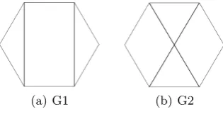
One of the problem with entropy defined in this way is that it captures only the local properties of a graph, and it is therefore sensitive to the degree distribution of the graph. For example, consider the non-isomorphic graphs in the Figure 1. The above two graphs are structurally different as G1 contains

(a) G1 (b) G2

Fig. 1.Two non-isomorphic graphs

two triangles whileG2 does not contain any triangle. However it can be shown

that, using Definition 2, the entropy for both the graphs is

If(G) =−

_2α16

2α16_{+ 4α}18log

_2α16

2α16_{+ 4α}18

+ 4α

18

2α16_{+ 4α}18log

_4α18

2α16_{+ 4α}18

Figure 2(a) plots the entropy of the two graphs as a function ofα.

(a) Path Length (b) Random Walk

Fig. 2.Entropy computed from different information functionals

3

Substructure based approach for Graph Entropy

To overcome the problems associated with the methods discussed above, we use random walks on a graph to define graph entropies. Motivated by Esterada’s Index (EI), we define the information functional based on closed random walks.

Definition 3 Let |Rk(vi, G)| denotes the number of random walks in graph G

of lengthk, starting from and ending at the nodevi. We define the information

functional as

fV_(v

i) :=αc1|R1(vi,G)|+c2|R2(vi,G)|+....+ck|Rk(vi,G)|

Note that if we put cn = _n1!, then the value in the exponent becomes equal to

Estrada’s Index (EI) [2].

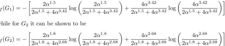
Using Definition 3 the entropy for graphG1of Figure 1 can be shown to be

If(G1) =−

_2α1.5

2α1.5_{+ 4α}3.42log

_2α1.5

2α1.5_{+ 4α}3.42

+ 4α

3.42

2α1.5_{+ 4α}3.42log

_4α3.42

2α1.5_{+ 4α}3.42

while forG2it can be shown to be

If(G2) =−

2α1.8

2α1.8_{+ 4α}2.68log

2α1.8

2α1.8_{+ 4α}2.68

+ 4α

2.68

2α1.8_{+ 4α}2.68log

4α2.68

2α1.8_{+ 4α}2.68

Figure 2(b) plots the entropies as a function of α for both graphs, which suggests that random walks are a more powerful tool for discriminating between different graph structures.

Our goal in this paper is to define graph entropy using the substructures in the graph. To this end, we decompose the graph into substructures and then use the frequency of a particular substructure to compute the information functional. We now propose a general framework to define entropy.

Definition 4 Given a graph G, we define the graph entropy as

If(G) =− n X

k=1

f(Sk) Pn

i=1f(Si)

logPnf(Sk) i=1f(Si)

(2)

whereSk represents the information functional computed fromkth substructure.

⊓ ⊔

There are a number of ways in which a graph can be decomposed and in-formation functionals can be defined. Here we use the coefficients of Ihara zeta function. The reason for using Ihara coefficients is that they are related to the number of simple cycles in the graphs, and hence can be used to gauge the cyclic complexity of a graph.

The Ihara zeta function associated to a finite connected graphGis defined to be a function ofu∈C_{with|u|sufficiently small by [13]}

ζG(u) = Y

c∈[C]

1−ul(c)−1 ₍₃₎

The product is over equivalence classes of primitive closed backtrackless, tail-less cyclesc = (v1, v2, v3, ..., vr =v1) of positive length rin G. Herel(c) represents

the length of the cycle.

The reciprocal of Ihara zeta function can also be written in the form of a determinant expression [14]

ζG(u) =

1

Lecture Notes in Computer Science 5

where T, the Perron-Frobenius operator, is the adjacency matrix of the oriented line graph of the original graph, andIis the identity matrix of size 2m. Heremis the number of edges in the original graph. The oriented line graph is constructed by first converting the graph into equivalent digraph, and then replacing each arc of the resulting digraph by a vertex. These vertices are connected if the head of one arc meets the tail of another while preventing backtracking, i.e., arcs corresponding to same edge are not connected.

Since the reciprocal of the Ihara zeta function can be written in the form of a determinant expression, therefore it can also express as a polynomial of degree at most 2. i.e.,

ζG(u)−1= det(I−uT) =c0+c1u+c2u2+c3u3+...+c2mu2m (5)

wherec0, c1, ..., c2mare called Ihara coefficients and are related to the frequencies

of simple cycles in the graph. In particular, it can be shown that ifGis a simple graph then c0 = 1, c1 = 0, c2 = 0. Furthermore, the coefficients c3, c4 and c5

are the negative of twice the number of triangles, squares, and pentagons in

G respectively. The coefficient c6 is the negative of the twice the number of

hexagons in G plus four times the number of pairs of edge disjoint triangles plus twice the number of pairs of triangles with a common edge, whilec7 is the

negative of the twice the number of heptagons inGplus four times the number of edge disjoint pairs of one triangle and one square plus twice the number of pairs of one triangle and one square that share a common edge [6, 7]. In [7], we have developed method that can be used to compute Ihara coefficients in a polynomial amount of time.

Definition 5 Let ci represents theithIhara coefficient. We define the

informa-tion funcinforma-tionals,f(ci), as

f(i) :=αkici_,

whereki are constants. ⊓⊔

Note that the first three Ihara coefficients are constants [6, 7], and therefore we can ignore these coefficients in our computation. Also, since the coefficient beyond the first few coefficients contain redundant information [7], therefore we only retain few coefficients and discard the remainder.

4

Experiments

4.1 Random Graphs

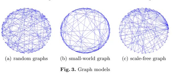
We commence by experimenting with the proposed method on synthetically generated graphs according to the following three models.

Erd˝os-R´enyi model(ER) [10]: AnERgraphG(n, p) is constructed by con-necting n vertices randomly with probability p. i.e., each edge is included in the graph with probability p independent from every other edge. These models are also calledrandom networks.

Watts and Strogatz model(WS) [11]: AW SgraphG(n, k, p) is constructed in the following way. First construct a regular ring lattice, a graph withn

vertices and each vertex is connected to k nearest vertices, k/2 on each side. Then for every vertex take every edge and rewire it with probabilityp. These models are also calledsmall-world networks.

Barab´asi-Albert model(BA) [12]: ABA graphG(n, n0, m) is constructed

by an initial fully connected graph withn0 vertices. New vertices are added

to the graph one at a time. Each new vertex is connected to m previous vertices with a probability that is proportional to the number of links that the existing nodes already have. These models are also calledscale-free networks.

Figure 6 shows an example of each of these models. We have generated 200

(a) random graphs (b) small-world graph (c) scale-free graph

Fig. 3.Graph models

graphs for each of these models with n = 21, 22,...,220. The parameters for these models were chosen in such a way that graphs with the same number of vertices have roughly the same number of edges. For ER graphs we choose p= 15/n, For W S graphs we choose k = 16 and p=.25, and forBA graphs we choose

n0= 9 andk= 8.

Next we compute the entropy of each graph using both the random walks and Ihara coefficients. We have used the coefficients of Ihara zeta function and closed random walks as information functional to compute entropy. For the Ihara coefficients, we have selected the first six coefficients starting for c3 to compute

Lecture Notes in Computer Science 7

For each graph, we have generated a feature vector of length 100. The feature vector is constructed by choosing different values ofαand computing information functional and the resulting entropy for each value ofα. In our case we have put

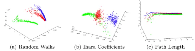
α = 0.1,0.2, ...,10. This transforms each graph into a feature vector in a 100 dimensional feature space. To visualise the results, we have performed Principal Component AnalysisPCAon the resulting feature vectors and embed the results in a three dimensional vector space.PCA is mathematically defined [17] as an orthogonal linear transformation that transforms the data to a new coordinate system such that the greatest variance by any projection of the data comes to lie on the first coordinate (called the first principal component), the second greatest variance on the second coordinate, and so on. Figure 4(a) shows the resulting embedding on the first three principal components for feature vectors computed using random walks, while Figure 4(b) shows the resulting embedding on the first three principal components for feature vectors computed using Ihara coefficients. To compare the results, we have also used the local information functional defined by Dehmer [1] that is computed from path lengths. Figure 4(c) shows the resulting embedding. The resulting embedding shows that the

(a) Random Walks (b) Ihara Coefficients (c) Path Length

Fig. 4.PCA_{embedding of different methods}

entropy computed from random walks gives best results. The Ihara coefficients on the other hand does not provide very good inter-class separation. This is due to the fact that graphs generated using random models have limited number of cycles. Figure also suggest that local information (path length) is not very helpful in distinguishing the different families of graphs.

4.2 Graphs extracted from COIL dataset

from the corresponding objects respectively. Next we used Dehmer’s

defini-(a) COIL (b) DT (c) GG (d) RNG

Fig. 5.COIL objects and their extracted graphs.

tion to compute the entropy of each graph extracted from each of the 72 views of all the 20 objects. We have used the coefficients of Ihara zeta function and closed random walks as information functional to compute entropy. For the Ihara coefficients, we have selected the first six coefficients starting for c3. To avoid

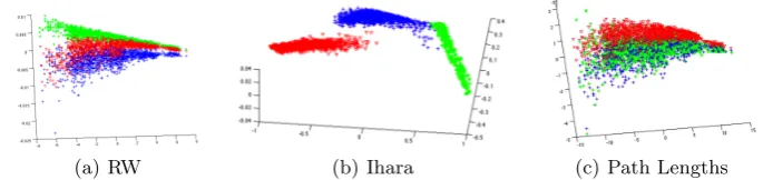
the scaling effect, the last three coefficients were multiplied with 1/|E|. For each graph, we have generated a signature of length 100 by puttingα= 0.1,0.2, ...,10. For random walk, we have selected random walk upto length 6. Each coefficient was multiplied with 1/k!, wherekis the length of the random walk. Finally, we have also used the local information functional defined by Dehmer to compute entropy. To compare the results, we have performed Principal Component Anal-ysisPCA, on the signatures obtained by choosing different values ofαfor each of these methods and embed the results in a three dimensional vector space. Fig-ure 4 compares the resulting embedding of the featFig-ure vectors on the first three principal components for all the three methods. It is clear from the figure that Ihara coefficients proves to be a powerful tool to distinguish graphs that exhibit a cyclic structure. On the other hand, the entropy computed from random walks and local paths is not very helpful in distinguishing these graphs.

(a) RW (b) Ihara (c) Path Lengths

Fig. 6.PCA embedding for COIL dataset

4.3 Time-varying Networks

Lecture Notes in Computer Science 9

an empirical value of 0.85 as a threshold value. This was done under the assump-tion that, at any given time, a particular stock must interact with another stock. A new network is generated by sliding the window of 1 day and repeating the process. In this way a total of 5977 time-varying networks are generated. Since the networks generated in this way have very limited number of prime cycles, We have used the entropy defined using closed random walks. We next applied PCA on the resulting signatures. Figure 7 shows the values of the eigenvector with the highest variance. The above result suggests that the proposed method

Fig. 7.Entropy computed from random walks on networks

is a very useful tool for detecting changes in a time evolving network. To com-pare these results, we have computed the entropy using path length as defined by Dehmer. Figure 8 shows the values of the first principal component, after applying PCA on the resulting signatures. This clearly suggests that entropies

Fig. 8.Entropy computed from path lengths usingj-sphere

defined using local structural properties are not very helpful to detect changes in a time evolving network.

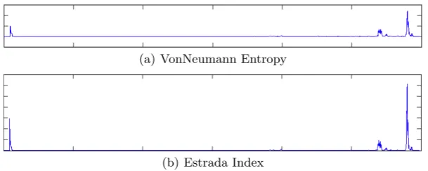
To compare the results, we have also computed the von Neumann entropy and the Estrada index of the evolving networks. Figure 9 shows the results.

(a) VonNeumann Entropy

(b) Estrada Index

Fig. 9.VonNeumann Entropy and Estrada Index for NYSE

5

Conclusion

a network). We have decomposed the graph into substructures and used the frequencies of these substructures to define entropy. We have also presented a generic framework that can be used to define graph entropy by decomposing the graph into substructures. Experiments were performed on numerous datasets including synthetic data, cyclic graphs, and time series data, and the results suggest that the proposed methods can be used to characterise the graphs (and networks) with very higher accuracy as compared to some of the other state-of-the-art methods.

References

1. Dehmer, M.: Information processing in complex networks: Graph entropy and in-formation functionals, Applied Math. and Comp., Vol 201, 2008, Pages 82-94. 2. Estrada, E.: Characterization of 3D molecular structure. Chemical Physics Letters,

Volume 319, Issues 5-6, 24 March 2000, Pages 713-718.

3. K¨orner, J.: Coding of an information source having ambiguous alphabet and the entropy of graphs. 6th Prague conference on information theory. 1973.

4. Kolmogorov, A.N.: Three approaches to the definition of the concept ?quantity of information? Probl. Peredachi Inf., 1965, Volume1, Issue1, Pages3?11

5. Chaitin, G. J. : On the Length of Programs for Computing Finite Binary Sequences Journal of the ACM, Volume 13 Issue 4, Oct. 1966.

6. Scott, G., Storm, C.: The coefficients of the Ihara zeta function, Involve - a journal of mathematics. Vol. 1 (2008), No. 2, 217?233.

7. Aziz, F., Wilson, R. C., Hancock, E. R.: Backtrackless Walks on a Graph. IEEE Trans. on Neural Netw. and Learning Systems, Volume 24, Issue 6, Pages 977-989. 8. Ren, P., Wilson, R.C., Hancock, E.R.: Graph Characterization via Ihara Coefficients. IEEE Transactions on Neural Networks, vol 22(2), 233 - 245, 29 November 2010. 9. Escolano, F., Hancock, E. R., Lozano, M.A.: Heat diffusion: Thermodynamic depth

complexity of networks. Phys. Rev. E, vol 85(3), Mar 2012.

10. Erd˜os, P., R´enyi A.: On the evolution of random graphs. Publications of the Math-ematical Institute of the Hungarian Academy of Sciences, 17-61 (1960).

11. Watts, D. J., Strogatz, S. H.: Collective dynamics of ’small-world’ networks. Na-ture, 440-442 (1998).

12. Barab´asi A., and Albert R.: Emergence of Scaling in Random Networks. Science 509-512 (1999).

13. Bass, H.: The Ihara-Selberg zeta function of a tree lattice. Int. J. Math., 1992, 717-797.

14. Kotani, M., Sunada, T.: Zeta function of finite graphs. Journal of Mathematics, University of Tokyo 7(1), 2000, pages 7-25.

15. Delaunay, B.: Sur la sphre vide, Izvestia Akademii Nauk SSSR, Otdelenie Matem-aticheskikh i Estestvennykh Nauk, 1934, 793800.

16. Toussaint, G.T.: The relative neighbourhood graph of a finite planar set, Pattern Recognition, 1980, 261 - 268.

17. Jolliffe, I. T.: Principal Component Analysis, Springer-Verlag, New York, 1986. 18. Gabriel, K. R., Sokal R. R.: A New Statistical Approach to Geographic Variation

Analysis, Systematic Zoology, 1969, 205-222.

19. Harris, C., Stephens, M.: A combined corner and edge detector, In Fourth Alvey Vision Conference, Manchester, UK, 1988, 147-151.