International Journal of Innovative Technology and Exploring Engineering (IJITEE) ISSN: 2278-3075, Volume-8 Issue-7, May, 2019
1835
Published By:
Blue Eyes Intelligence Engineering & Sciences Publication
Retrieval Number: G6103058719 /19©BEIESP
Abstract: This paper investigates the provision of buffer mechanism impact for interrupted secondary users using analytical finite time dependent queuing model. The main focus of the research area in Cognitive Radio Networks(CRN) is the spectrum access management of the secondary users along with interrupted secondary users, because the secondary users play key role for getting maximum revenue of service providers with opportunistic spectrum access. During the transmission period of secondary users, the handoffs occurred due to primary user arrivals when all channels are busy. The primary users arrival rate, the state of all channels busy are fluctuated from time to time. In this paper, to resolve these timely varying problems with a two fold. (i) provision of buffer for the interrupted secondary users (ii) transition analysis is carried out to identify transition behavior of interrupted secondary users. For achieving these objectives, the CRN transmission process modeled as multi channel with finite buffer queueing model and differential equations are derived. Important performance metrics are evaluated based on these derived equations and numerical illustration is carried out. The analytical results presented as tables and graphs and conclusions are drawn.
Index Terms: Cognitive radio networks, M/M/C/K, queue length, throughput, blocking probability
I. INTRODUCTION
The usage of wireless devices is exponentially increasing with the evolution of Cognitive Radio technology. This CR technology focuses on sensing and sharing the white spaces of the spectrum with intelligence by developing a new type of network called as Cognitive Radio Networks. By The white spaces and related Statistics of spectrum utilization showing that poor utilization of the spectrum is taking place even the demand is increasing. To minimize the white space and effective usage of the spectrum, so many paradigms are evolved like overlay, interweaving and underlay. For effective usage of the spectrum, the interweaving paradigm is adapted where each user is given an opportunity to best utilize the complete resources whenever the spectrum seems to have a white space.
Revised Manuscript Received on May 10 ,2019
B.B.V. Satya Vara Prasad, Research Scholar Department of CSE, Acharya Nagarjuna University, Guntur, India & Assistant Professor in KLEF, Vijayawada, India
B. Basaveswara Rao, University Computer Centre, Acharya Nagarjuna University, Guntur, India.
V. Vasanta Kumar, Professor& Head of the Department, Department of Mathematics, K L E F, Vijayawada, India.
K. Chandan, Professor, Department of Statistics, Acharya Nagarjuna University, Guntur, India.
The Primary Users (PU) or licensed users will be given high priority for reserving and use of the spectrum and when an underutilization takes place, the secondary or unlicensed users (SU) will be given an opportunity for using the spectrum resources under the supervision of a service provider (SP). The secondary users are allowed to utilize all the resources completely and effectively like a primary user whenever a channel is free. The main research area is to fully utilize the limited spectrum with effectively and share the spectrum among the secondary users coexists in this spectrum band.
In this interweaving scenario, the secondary users in service will be interrupted by the primary users when no other channels are free. Interweaving paradigm is showing a great concern of providing service in effective manner but the problem can be expected is the interruptions to secondary users in utilization because of the arrivals of primary users when the channels are busy. To handle the issue of interrupted users, buffers can be used to temporarily hold them for resuming the services to interrupted secondary users until the channels become free. In this paper, a comparative study of service provision to secondary users with and without buffers is carried. There are several authors addressing this issue and proposed models with queuing and without queuing.
The categorization of users is not done and is considered only with finite population is studied with continuous Markov chain(CTMC) [1] is the basis for considering the performance parameters. The M/M/1 model proposed in [2] is not considered for this problem even it provides the access based on priorities as C channels are assumed in this paper. Buffer related issues are considered for service rate improvement for secondary users is discussed in [3] but is implemented with forced policies. The effective usage of buffers is not clearly explained with analytical model [4].
Admission control policies of secondary users is discussed but with Dynamic Programming instead of M/M/C/K Model [5]. The prior decision to join in the service or not is considered in [6] but not discussed the issues of usage of buffers for interrupted services. Even the parameter throughput [7] is considered for large population of secondary users, but no clear explanation and usage with M/M/C/K model is available. Queuing analysis is carried with low and high priority queues [8] but is limited to underlay networks which is not effective in spectrum utilization compared with interweaving paradigm. Quality of service related issues with primary and secondary user delays [9] is useful but not effective with M/D/1 model. Feedback based analysis over access
control mechanism is also
Transient Analysis of Interrupted Secondary
Users With the Provision of Finite Buffer
Transient Analysis of Interrupted Secondary Users With the Provision of Finite Buffer
useful [10] but not available with M/M/C/K model. Most of the research works are not covered the interweaving paradigm with limited buffer constraint and they are considered the deterministic services. To fulfill this gap, the study is carried out. The paper objectives are as follows:
To provide an analytical model for interrupted secondary users with buffer mechanism using M/M/C/K where K is buffer capacity and C is no. of channels.
To derive differential equations for finding performance metrics like queue length, waiting time and delays of users
Finally, numerical illustration is carried out for multiple channels with finite buffer size and draw conclusions
The remaining paper is organized as follows. In Section 2, the relevant literature is presented precisely. The mathematical model covering generalized equations with all possible cases and the transitional state diagram are explained in Section 3. The numerical analysis provided in Section 4. Finally, results and conclusions are given in Section 5.
II. LITERATURESURVEY
Cognitive Radio Networks (CRN) deals with the Spectrum efficient usage issues in the real world. The buffering and switching scheme for admission control were discussed [13] for opportunistic usage of the spectrum but with multi-dimensional Markov chain model. Priority Queueing issues are introduced with [11] but it is limited to Underlay Cognitivie Networks. The Priority Queueing Analysis for quality improvement [12] is carried but limited to Markov chains. Multi-channel Cognitive Radio Networks – modeling , analysis and synthesis [15] with a mixed strategy with CTMC unable to cover opportunistic access issues clearly. Spectrum sharing with buffering in Cognitive Radio Networks[14] is modeled but unable to clearly explain with the designed model. To derive the parameters Throughput and Delay [16] , the cooperative access issues are discussed but unable to cover the handoff mechanisms in detail. The opportunistic access optimization with primary queue stability constraint mechanism with feedback option [17] is discussed but not focused on buffering mechanisms for secondary users.
III. INTERRUPTED SECONDARY USERS BUFFER QUEUING
MODEL (ISUBQM)
Different authors proposed and analyzed Cognitive Radio Networks with M/D/1 and other queuing models for obtaining the optimum spectrum usage by both types of users. But many of them have not considered the idea of creating a buffer for interrupted secondary users. In this work, an attempt has been made to analyze the CRN with a dedicated buffer for the interrupted secondary users.
To evaluate the dynamic behavior of the CRN with buffer mechanism, the M/M/C/K queuing model is proposed and analyzed for the different performance metrics with two channels supported by one buffer for the interrupted
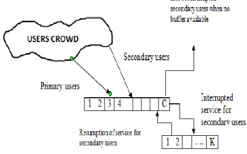
[image:2.595.322.567.142.294.2]secondary users. The two channels option is considered to minimize the complexity of the problem. This model covers the users population containing both types of users: Primary and Secondary who are in need of Service. The generalized CRN with C channels and K buffers is depicted in the following figure1.
Figure 1: CRN with C channels and K buffers for Interrupted Secondary Users
Assumptions:
Both primary and secondary users arrival rate follow Poisson distribution.
Both users service time follow exponential distribution with same service rate.
High priority is given to Primary Users.
Upon arrival of Primary user, if all channels are occupied by both users, then the Secondary user has to vacate channel and has to wait in the buffer.
When any channel becomes available, interrupted secondary user may resume the service.
The number of channels C is equivalent to buffer size k because this analytical study restricted to interrupted secondary users utilize the buffer when the primary user arrives and all channels are occupied. At any time , the number of interrupted secondary users will not exceed the no. of channels. So, the buffer size is limited to channel size for efficient memory utilization.
Notations:
: - Primary user arrival rate : - Secondary user arrival rate : - Service rate
n : - Number of channels reserved for providing service k : - Buffer size
np : - Number of channels occupied by primary users ns : - Number of channels occupied by secondary users L : - Average length of the Queue
Wp : - Waiting time of primary users Ws : - Waiting time of secondary users Pl : - Expected primary user loss Sl : - Expected Secondary user loss T : - Throughput of the
System
International Journal of Innovative Technology and Exploring Engineering (IJITEE) ISSN: 2278-3075, Volume-8 Issue-7, May, 2019
1837
Published By:
Blue Eyes Intelligence Engineering & Sciences Publication
Retrieval Number: G6103058719 /19©BEIESP
Ptput: - Throughput of Primary Users
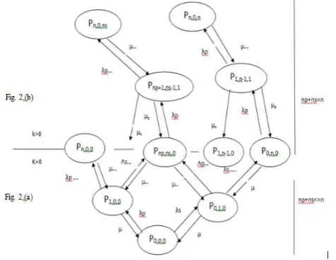
[image:3.595.53.291.192.376.2]The state diagram, Figure2 was shown with two parts . Figure 2.(a) and Figure 2.(b) are drawn showing the all possibilities of state changes with the arrivals and departures of both primary and secondary users. Figure 2.(a) covers the case of no requirement of usage of buffer for any user as the available channels are sufficient to avail service. State diagram 2.(b) covers the scenario of occupying buffer by secondary user satisfying the constraints. The buffer usage is restricted to interrupted secondary users only. The buffer size is maintained as k=n.
Figure 2: State transition diagram for channels c=n and buffer size k=n
Let P np, ns, k be the probability of occurrence of a state where np represents the no. of channels in use by primary users and ns represents the no. of channels in use by secondary users and k represents the buffer occupied by no. of interrupted secondary users for waiting the resumption of service.
The differential difference equations for all possible cases considered for availing the service are
Case 1: When all channels are free,
--- (1) Case 2: When channels are occupied by primary users only and vacant channels are available,
i.e. 1<= np< n, ns=0, k=0
--- (2)
Case 3: When all channels are occupied by primary users, i.e. np = n, ns=0, k=0
-- (3)
Case 4: When channels are occupied by secondary users only and vacant channels are still available,
i.e. 1<= ns< n, np=0, k=0
--- (4) Case 5: When channels are occupied by both primary and secondary users and some channels are still vacant, i.e. 1<= np + ns < n , np >0, ns>0, k=0
--- (5) Case 6: When all channels are occupied by both primary and secondary users & buffer is empty,
i.e. 1 <= ns <= n-1, 1<=np <= n-ns, k=0
- --- (6)
Case 7: When all channels are occupied by both users and buffer is partially filled with secondary users,
i.e. np +ns=n where 1<= np, ns <n & 1<= k < np
+ --- (7)
Case 8: When all channels are occupied by secondary users and the buffer is empty,
--- (8)
Case 9: When all channels are occupied by primary users and the buffer is partially/completely occupied,
i.e. np=n, k< =np
--- (9)
Case 10: When all channels are occupied by both users and the buffer is occupied as k=np,
i.e. np +ns=n where 1<= np, ns <n & k = np
--- (10)
IV. PERFORMANCEANALYSIS
In this section various performance metrics: Expected Queuing Delay, Throughput, Average Response Time and Packet Dropping Probability for both the users are presented based on the model explained above.
a.
Queue Length (L) :Transient Analysis of Interrupted Secondary Users With the Provision of Finite Buffer
The Queue Length is defined for ISUBQM based on n n-i n
L = ∑ ∑ ∑ ( i + j + k ) Pi,j,k xiyjzk i=0 j=0 k=0
b.
Waiting Time (W) :The time taken by the users to wait in buffer to utilize the channel service is called waiting time.
W= L / λ where λp+λs
c.
Blocking Probability of Primary User (Ploss) :When primary user arrives, the secondary user if any in service will be interrupted for providing service to primary user. When all the channels are occupied by primary users, the new primary user will not be given service and this situation will give the blocking probability of primary user. It can be shown as
n Ploss = ( ( / )n / n! ) / ( ∑ (( / )i / i! ) i=0
d.
Blocking Probability of Secondary User (Sloss) :When the secondary users are not given to utilize the channel service when all the channels are occupied , the blocking probability is given as
n Sloss = ( ( / )n / n! ) / ( ∑ (( / )i / i! ) i=0
e.
ThroughputThroughput is the maximum rate of production or the maximum rate at which something can be processed. When
is considered as the arrivals of users, the final throughput can be considered as
T = λp- λp*{Total probability of primary users unable to get the service} + - *{Total probability of secondary users unable to get the service}
Numerical Illustration:
In this section, using MAT Lab, the performance metrics are evaluated as presented in the above section for various values of , n and k=n. The numerical illustrations are carried out in two scenarios, they are time-dependent performance metrics and time independent performance metrics i.e. both users’ loss probabilities.
Case-1: Time-Dependent Performance Metrics:
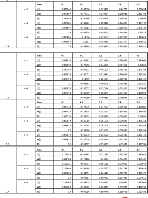
values are raised from 0.4 to 0.6 for different values of ranging from 0.4 to 0.7 are taken for calculating time dependent performance metrics. Different cases of varying the number of channels is shown. For all these calculations, the value is taken as 1.2 to 1.4.
Calculations of Queue Length-L(t), Waiting Time-W(t) and Secondary user Throughput T(t) for different values of
Transient Analysis of Interrupted Secondary Users With the Provision of Finite Buffer
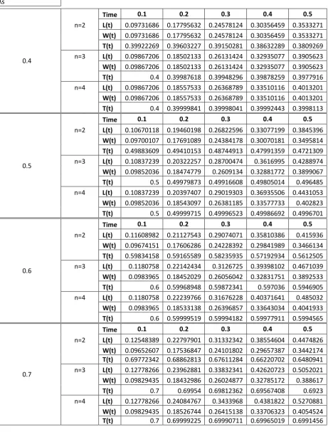
Table 1: Results of performance parameters L, W and T at different values of Time 't' when λp= 0.4 and µ=1.3
λs
0.4
Time 0.1 0.2 0.3 0.4 0.5
n=2 L(t) 0.078246 0.143818 0.199467 0.24723 0.288634
W(t) 0.097807 0.179772 0.249334 0.309038 0.360793
T(t) 0.399495 0.397386 0.394328 0.390759 0.38697
n=3 L(t) 0.079086 0.148282 0.209442 0.264013 0.313139
W(t) 0.098857 0.185353 0.261802 0.330016 0.391424
T(t) 0.4 0.399934 0.399722 0.399336 0.39878
n=4 L(t) 0.079086 0.14856 0.210655 0.267006 0.318829
W(t) 0.098857 0.1857 0.263319 0.333757 0.398536
T(t) 0.4 0.399999 0.399992 0.399967 0.399916
0.5
Time 0.1 0.2 0.3 0.4 0.5
n=2 L(t) 0.087838 0.161187 0.223294 0.276535 0.322668
W(t) 0.097598 0.179096 0.248105 0.307262 0.35852
T(t) 0.499197 0.495873 0.491104 0.485593 0.479792
n=3 L(t) 0.088878 0.166671 0.235471 0.296918 0.352306
W(t) 0.098753 0.18519 0.261634 0.329909 0.391452
T(t) 0.5 0.499883 0.499508 0.498834 0.497869
n=4 L(t) 0.088878 0.167057 0.237144 0.301013 0.360034
W(t) 0.098753 0.185619 0.263494 0.334458 0.400038
T(t) 0.5 0.499999 0.499983 0.499934 0.499835
0.6
Time 0.1 0.2 0.3 0.4 0.5
n=2 L(t) 0.097434 0.178575 0.247167 0.305916 0.356806
W(t) 0.097434 0.178575 0.247167 0.305916 0.356806
T(t) 0.598799 0.593872 0.586876 0.578871 0.57052
n=3 L(t) 0.098672 0.185065 0.261506 0.329823 0.391464
W(t) 0.098672 0.185065 0.261506 0.329823 0.391464
T(t) 0.6 0.599806 0.599189 0.598089 0.596533
n=4 L(t) 0.098672 0.185576 0.263699 0.335147 0.401441
W(t) 0.098672 0.185576 0.263699 0.335147 0.401441
T(t) 0.6 0.599997 0.599969 0.59988 0.599701
0.7
Time 0.1 0.2 0.3 0.4 0.5
n=2 L(t) 0.107034 0.195985 0.271083 0.335359 0.391014
W(t) 0.097304 0.178168 0.24644 0.304871 0.355467
T(t) 0.698285 0.691311 0.681515 0.670416 0.658942
n=3 L(t) 0.108469 0.203468 0.287552 0.362738 0.430624
W(t) 0.098608 0.184971 0.261411 0.329761 0.391476
T(t) 0.7 0.699694 0.698733 0.697037 0.694659
n=4 L(t) 0.108469 0.204119 0.290322 0.36941 0.443042
W(t) 0.098608 0.185563 0.263929 0.335827 0.402765
International Journal of Innovative Technology and Exploring Engineering (IJITEE) ISSN: 2278-3075, Volume-8 Issue-7, May, 2019
1839
Published By:
Blue Eyes Intelligence Engineering & Sciences Publication
[image:7.595.43.498.121.664.2]Retrieval Number: G6103058719 /19©BEIESP
Table 2: Results of performance parameters L, W and T at different values of Time 't' when λp= 0.5 and µ=1.3
λs
0.4
Time 0.1 0.2 0.3 0.4 0.5
n=2 L(t) 0.08778814 0.16092171 0.22269827 0.27552105 0.3211642
W(t) 0.09754238 0.1788019 0.24744252 0.3061345 0.3568491
T(t) 0.39936763 0.39674906 0.39299209 0.38865161 0.3840857
n=3 L(t) 0.08887776 0.16665396 0.23539716 0.29673541 0.3519566
W(t) 0.09875307 0.18517106 0.2615524 0.32970601 0.3910629
T(t) 0.4 0.3999087 0.39961576 0.39908867 0.3983357
n=4 L(t) 0.08887776 0.16705679 0.23714046 0.30099664 0.3599923
W(t) 0.09875307 0.18561865 0.2634894 0.33444071 0.3999914
T(t) 0.4 0.39999894 0.39998688 0.39994897 0.3998716
0.5
Time 0.1 0.2 0.3 0.4 0.5
n=2 L(t) 0.097278 0.17793582 0.24584827 0.30379947 0.3538187
W(t) 0.097278 0.17793582 0.24584827 0.30379947 0.3538187
T(t) 0.499027 0.49503402 0.48936444 0.48287696 0.4761117
n=3 L(t) 0.09862377 0.18495128 0.26126876 0.32939046 0.390759
W(t) 0.09862377 0.18495128 0.26126876 0.32939046 0.390759
T(t) 0.5 0.49984519 0.49935357 0.49847762 0.4972374
n=4 L(t) 0.09862377 0.18550408 0.26363845 0.33513343 0.4015058
W(t) 0.09862377 0.18550408 0.26363845 0.33513343 0.4015058
T(t) 0.5 0.49999801 0.49997543 0.49990521 0.4997633
0.6
Time 0.1 0.2 0.3 0.4 0.5
n=2 L(t) 0.10677166 0.19497345 0.26905573 0.33217719 0.3866159
W(t) 0.09706514 0.17724859 0.24459611 0.30197926 0.351469
T(t) 0.59858216 0.59281586 0.58471359 0.57553197 0.5660413
n=3 L(t) 0.10837239 0.20325204 0.28713214 0.36201203 0.4294912
W(t) 0.09852036 0.18477458 0.26102922 0.32910184 0.3904466
T(t) 0.6 0.59975271 0.59897542 0.59760415 0.5956802
n=4 L(t) 0.10837239 0.20397474 0.2902015 0.3693888 0.4431927
W(t) 0.09852036 0.18543158 0.26381954 0.335808 0.4029025
T(t) 0.6 0.59999648 0.59995705 0.59983562 0.5995925
0.7
Time 0.1 0.2 0.3 0.4 0.5
n=2 L(t) 0.11627027 0.21203707 0.29231891 0.36064069 0.4195227
W(t) 0.09689189 0.17669756 0.24359909 0.30053391 0.3496023
T(t) 0.69801723 0.69002595 0.67891496 0.6664464 0.6536727
n=3 L(t) 0.11812401 0.22155841 0.31299284 0.3946105 0.4681697
W(t) 0.09843668 0.18463201 0.26082737 0.32884209 0.3901414
T(t) 0.7 0.69962303 0.69845036 0.69640217 0.6935549
n=4 L(t) 0.11812401 0.22247042 0.31683126 0.40376106 0.4850432
W(t) 0.09843668 0.18539202 0.26402605 0.33646755 0.4042027
Transient Analysis of Interrupted Secondary Users With the Provision of Finite Buffer
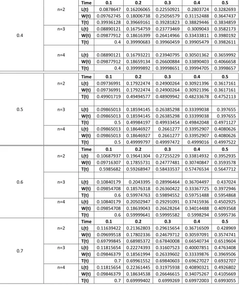
Table 3: Results of performance parameters L, W and T at different values of Time 't' when λp= 0.6 and µ=1.3
λs
0.4
Time 0.1 0.2 0.3 0.4 0.5
n=2 L(t) 0.09731686 0.17795632 0.24578124 0.30356459 0.3533271
W(t) 0.09731686 0.17795632 0.24578124 0.30356459 0.3533271
T(t) 0.39922269 0.39603227 0.39150281 0.38632289 0.3809269
n=3 L(t) 0.09867206 0.18502133 0.26131424 0.32935077 0.3905623
W(t) 0.09867206 0.18502133 0.26131424 0.32935077 0.3905623
T(t) 0.4 0.39987618 0.39948296 0.39878259 0.3977916
n=4 L(t) 0.09867206 0.18557533 0.26368789 0.33510116 0.4013201
W(t) 0.09867206 0.18557533 0.26368789 0.33510116 0.4013201
T(t) 0.4 0.39999841 0.39998041 0.39992443 0.3998113
0.5
Time 0.1 0.2 0.3 0.4 0.5
n=2 L(t) 0.10670118 0.19460198 0.26822596 0.33077199 0.3845396
W(t) 0.09700107 0.17691089 0.24384178 0.30070181 0.3495814
T(t) 0.49883609 0.49410153 0.48744913 0.47991359 0.4721309
n=3 L(t) 0.10837239 0.20322257 0.28700474 0.3616995 0.4288974
W(t) 0.09852036 0.18474779 0.2609134 0.32881772 0.3899067
T(t) 0.5 0.49979873 0.49916608 0.49805014 0.496485
n=4 L(t) 0.10837239 0.20397407 0.29019303 0.36935506 0.4431053
W(t) 0.09852036 0.18543097 0.26381185 0.33577733 0.402823
T(t) 0.5 0.49999715 0.49996523 0.49986692 0.4996701
0.6
Time 0.1 0.2 0.3 0.4 0.5
n=2 L(t) 0.11608982 0.21127543 0.29074071 0.35810386 0.415936
W(t) 0.09674151 0.17606286 0.24228392 0.29841989 0.3466134
T(t) 0.59834158 0.59165589 0.58235935 0.57192934 0.5612505
n=3 L(t) 0.1180758 0.22142434 0.3126725 0.39398102 0.4671039
W(t) 0.0983965 0.18452029 0.26056042 0.32831751 0.3892533
T(t) 0.6 0.59968948 0.59872341 0.597036 0.5946905
n=4 L(t) 0.1180758 0.22239766 0.31676228 0.40371641 0.485032
W(t) 0.0983965 0.18533138 0.26396857 0.33643034 0.4041933
T(t) 0.6 0.59999519 0.59994182 0.59977911 0.5994565
0.7
Time 0.1 0.2 0.3 0.4 0.5
n=2 L(t) 0.12548389 0.22797901 0.31332342 0.38554604 0.4474826
W(t) 0.09652607 0.17536847 0.24101802 0.29657387 0.3442174
T(t) 0.69772342 0.68862813 0.67611284 0.66220702 0.6480941
n=3 L(t) 0.12778266 0.23962881 0.33832341 0.42620723 0.5052021
W(t) 0.09829435 0.18432986 0.26024877 0.32785172 0.388617
T(t) 0.7 0.69954 0.69812362 0.69567408 0.6923
n=4 L(t) 0.12778266 0.24084767 0.3433968 0.4381822 0.5270881
W(t) 0.09829435 0.18526744 0.26415138 0.33706323 0.4054524
International Journal of Innovative Technology and Exploring Engineering (IJITEE) ISSN: 2278-3075, Volume-8 Issue-7, May, 2019
1841
Published By:
Blue Eyes Intelligence Engineering & Sciences Publication
[image:9.595.49.529.130.705.2]Retrieval Number: G6103058719 /19©BEIESP
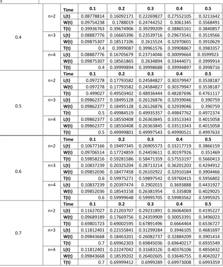
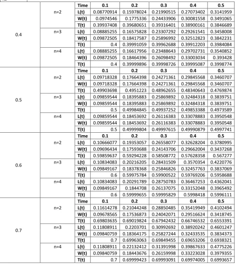
Table 4: Results of performance parameters L, W and T at different values of Time 't' when λp= 0.5 and µ=1.2
λs
0.4
Time 0.1 0.2 0.3 0.4 0.5
n=2 L(t) 0.0878647 0.16206065 0.22550921 0.2803724 0.3282693
W(t) 0.09762745 0.18006738 0.25056579 0.31152488 0.3647437
T(t) 0.39936128 0.39669161 0.39281823 0.38829446 0.3834859
n=3 L(t) 0.08890121 0.16754759 0.23773469 0.3009043 0.3582173
W(t) 0.09877912 0.18616399 0.26414966 0.33433811 0.3980192
T(t) 0.4 0.39990683 0.39960459 0.39905479 0.3982611
n=4 L(t) 0.08890121 0.16793221 0.23940795 0.30501362 0.3659992
W(t) 0.09877912 0.18659134 0.26600884 0.33890403 0.4066658
T(t) 0.4 0.39999892 0.39998651 0.39994705 0.3998657
0.5
Time 0.1 0.2 0.3 0.4 0.5
n=2 L(t) 0.09736991 0.17922474 0.24900264 0.30921396 0.3617161
W(t) 0.09736991 0.17922474 0.24900264 0.30921396 0.3617161
T(t) 0.49901719 0.49494577 0.48909942 0.48233678 0.4752113
n=3 L(t) 0.09865013 0.18594145 0.26385298 0.33399038 0.397655
W(t) 0.09865013 0.18594145 0.26385298 0.33399038 0.397655
T(t) 0.5 0.49984197 0.49933454 0.49842048 0.4971127
n=4 L(t) 0.09865013 0.18646927 0.2661277 0.33952907 0.4080626
W(t) 0.09865013 0.18646927 0.2661277 0.33952907 0.4080626
T(t) 0.5 0.49999797 0.49997472 0.4999016 0.4997522
0.6
Time 0.1 0.2 0.3 0.4 0.5
n=2 L(t) 0.10687937 0.19641304 0.27255229 0.33814932 0.3952935
W(t) 0.09716307 0.17855731 0.24777481 0.30740847 0.3593578
T(t) 0.5985682 0.59268947 0.58433537 0.57476534 0.5647712
n=3 L(t) 0.10840179 0.2043395 0.28996464 0.36704497 0.437024
W(t) 0.09854708 0.18576318 0.26360422 0.33367725 0.3972946
T(t) 0.6 0.59974763 0.59894552 0.59751488 0.5954868
n=4 L(t) 0.10840179 0.20502947 0.29291091 0.37415936 0.4502925
W(t) 0.09854708 0.18639043 0.26628264 0.34014488 0.4093568
T(t) 0.6 0.59999641 0.59995582 0.5998294 0.5995736
0.7
Time 0.1 0.2 0.3 0.4 0.5
n=2 L(t) 0.11639422 0.21362803 0.29615654 0.36716509 0.428969
W(t) 0.09699518 0.17802336 0.24679712 0.30597091 0.3574741
T(t) 0.69799845 0.68985372 0.67840008 0.66540734 0.6519604
n=3 L(t) 0.11815654 0.22274393 0.31607523 0.40007851 0.4763408
W(t) 0.09846379 0.18561994 0.26339602 0.33339876 0.3969506
T(t) 0.7 0.69961552 0.69840603 0.69627027 0.6932707
n=4 L(t) 0.11815654 0.22361445 0.31975938 0.40890321 0.4926802
W(t) 0.09846379 0.18634538 0.26646615 0.34075267 0.4105669
Transient Analysis of Interrupted Secondary Users With the Provision of Finite Buffer
Table 5: Results of performance parameters L, W and T at different values of Time 't' when λp= 0.5 and µ=1.4
λs
0.4
Time 0.1 0.2 0.3 0.4 0.5
n=2 L(t) 0.08770914 0.15978024 0.21990515 0.27073402 0.3141959
W(t) 0.0974546 0.1775336 0.24433906 0.30081558 0.3491065
T(t) 0.39937408 0.39680651 0.39316401 0.38900161 0.3846689
n=3 L(t) 0.08885255 0.16575828 0.23307292 0.29261541 0.3458008
W(t) 0.09872505 0.18417587 0.25896992 0.32512823 0.3842231
T(t) 0.4 0.39991059 0.39962688 0.39912203 0.3984084
n=4 L(t) 0.08885255 0.16617956 0.23488643 0.29702731 0.3540852
W(t) 0.09872505 0.18464396 0.26098492 0.33003034 0.393428
T(t) 0.4 0.39999896 0.39998726 0.39995087 0.3998774
0.5
Time 0.1 0.2 0.3 0.4 0.5
n=2 L(t) 0.09718328 0.17664398 0.24271361 0.29845568 0.3460707
W(t) 0.09718328 0.17664398 0.24271361 0.29845568 0.3460707
T(t) 0.49903698 0.4951223 0.48962655 0.48340643 0.4769874
n=3 L(t) 0.09859544 0.18395883 0.25869892 0.32484318 0.3839751
W(t) 0.09859544 0.18395883 0.25869892 0.32484318 0.3839751
T(t) 0.5 0.49984845 0.49937252 0.49853388 0.4973589
n=4 L(t) 0.09859544 0.18453692 0.26116383 0.33078883 0.3950548
W(t) 0.09859544 0.18453692 0.26116383 0.33078883 0.3950548
T(t) 0.5 0.49999804 0.49997615 0.49990879 0.4997741
0.6
Time 0.1 0.2 0.3 0.4 0.5
n=2 L(t) 0.10666077 0.19353057 0.26558077 0.32628204 0.3780995
W(t) 0.09696434 0.17593688 0.24143706 0.29662004 0.3437268
T(t) 0.59859637 0.59294228 0.58508772 0.57628358 0.567277
n=3 L(t) 0.10834083 0.20216205 0.28431509 0.3570354 0.4220776
W(t) 0.09849167 0.18378368 0.25846826 0.32457763 0.3837069
T(t) 0.6 0.59975784 0.59900522 0.59769206 0.5958688
n=4 L(t) 0.10834083 0.20291789 0.28750783 0.36467253 0.4362041
W(t) 0.09849167 0.1844708 0.26137075 0.33152048 0.3965492
T(t) 0.6 0.59999655 0.59995829 0.5998418 0.5996111
0.7
Time 0.1 0.2 0.3 0.4 0.5
n=2 L(t) 0.11614278 0.21044248 0.28850485 0.35419949 0.4102494
W(t) 0.09678565 0.17536873 0.24042071 0.29516624 0.3418745
T(t) 0.69803635 0.69019824 0.67942432 0.66746532 0.6553391
n=3 L(t) 0.11808911 0.2203701 0.30992692 0.38920242 0.4601247
W(t) 0.09840759 0.18364175 0.25827244 0.32433535 0.3834373
T(t) 0.7 0.69963063 0.69849455 0.69653206 0.6938321
n=4 L(t) 0.11808911 0.22132412 0.31391998 0.39867633 0.4775226
W(t) 0.09840759 0.18443676 0.26159998 0.33223028 0.3979355
International Journal of Innovative Technology and Exploring Engineering (IJITEE) ISSN: 2278-3075, Volume-8 Issue-7, May, 2019
1843
Published By:
Blue Eyes Intelligence Engineering & Sciences Publication
Retrieval Number: G6103058719 /19©BEIESP
Based on values derived above , when graphs are plotted for different arrival rates of secondary users with n channels, the queue length and throughput parameters values can be observed as
For the performance parameter Queue Length(L) :
Primary User Arrival Rate is taken on X-axis
1. Based on the calculated values for Queue Lengths , a graph is plotted by considering primary user arrival rate (λp) on X-axis at different values of number of channels (n) and Secondary user arrival rates (λs) at the fixed interval 0.3 with service rate(µ) as 1.3.
Figure.3.1: L Vs. λp at fixed µ, t
It is observed that the queue lengths are increasing w increase in values of parameters λp, λs and n respectively at fixed service rate.
2. When a graph is plotted by considering primary user arrival rate on X-axis at regular time intervals for fixed secondary user arrival rate (λs=0.5) with three channels(n=3) at different service rates(µ) ranging from 1.2 to 1.4 at differhent time intervals,it can be shown as
Fig.3.2: L Vs. λp at fixed λs, n
It is observed that the queue length is increasing as the increase in primary user arrival rate or time interval observed and at the same time , with the increase in service rate, decrease in queue length is observed at different time intervals for the same primary user arrival rate.
Secondary user arrival rate is fixed on X-axis
1.When a graph is plotted by considering secondary user arrival rate on X-axis at fixed time interval 0.3 with the service rate 1.3 for primary user arrival rate ranging from 0.4
to 0.6
Figure.4.1: L Vs. λs at fixed µ, t
The increase in queue length is observed with the increase in either secondary / primary user arrival rate or no. of channels or both at fixed service rate.
2. When a graph is plotted by considering secondary user arrival rate on X-axis at fixed primary user arrival rate as 0.5 with a system having channels , n=3 , the increase in service rates at regular time intervals can be shown as
Transient Analysis of Interrupted Secondary Users With the Provision of Finite Buffer
It is observed that the increase in queue lengths takes place when time progresses and at a fixed time interval point, the increase in service rate causes slight decrease in Queue Length.
Service rate is fixed on X-axis
1. When a graph is plotted by considering service rate on X-axis for different queue lengths at time interval 0.3 with fixed λp=0.5 for different λs varying from 0.4 to 0.7 for different no. of channels, it is shown as
Figure.5.1: L Vs. µ at fixed λp, t
It is observed a slight decrease in queue lengths with the increase in service rate (µ) and when the no. of channels raising from 3 to 4, the queue length values shows no marginal decrease in Queue length.
2. When a graph is plotted over different service rates for a system with three channels having constant secondary user arrival rate as λs=0.5 for different primary user arrival rates, it can be shown as
Figure.5.2: L Vs. µ at fixed λs, n
It is observed that as the time progresses, the queue length differences increases at fixed primary user arrival rate (λp)
and the increase in queue length is observed with the increase in λp.
No. of channels is fixed on X-axis
1. When a graph is drawn with no. of channels (n) as X-axis for various values of primary and secondary user arrival rates at the fixed time interval t=0.3 with service rate µ=1.3, it is shown
Figure.6.1: L Vs. n at fixed µ, t
It is observed that queue length increases if any of the arrival rates, λp or λs increases and it also observed that the increase in either λp or λs by fixing one of them is same.
2. When a graph is plotted with no. of channels(n) as X-axis at constant arrival rates of primary and secondary users at regular time intervals with service rates ranging from 1.2 to 1.4, it can be shown as
Figure.6.2: L Vs. n at fixed λp,λs
International Journal of Innovative Technology and Exploring Engineering (IJITEE) ISSN: 2278-3075, Volume-8 Issue-7, May, 2019
1845
Published By:
Blue Eyes Intelligence Engineering & Sciences Publication
Retrieval Number: G6103058719 /19©BEIESP
Time interval value is fixed on X-axis:
1. When a graph is plotted with time interval as X-axis at constant service rate, µ=1.3 and primary user arrival rate fixed at λp=0.5 for different channels and different secondary user arrival rates, it can be shown as
Figure.7.1: L Vs. t at fixed µ, λp
It is observed that the increase in queue length will take place the increase in no. of channels(n) value or increase in secondary user arrival rate (λs) takes place.
2. When a graph is plotted with no. of channels, n as X-axis for a system with no. of channels, n=3 and secondary user arrival rate as (λs=0.5) at different service rate with primary user arrival rate ranging from 0.4 to 0.6, it can be shown as
Figure.7.2: L Vs. t at fixed µ, λp
The increase in queue length is taking place as λp increases and at a particular λp, the queue length is decreasing as the service rate increases.
For the performance parameter Secondary user
Throughput(Stput) :
Primary user arrival rate is fixed on X-axis
1. When a graph is drawn by considering secondary user arrival rate fixed at 0.5 with a 3-channel system at various service rates for regular intervals with primary user arrival rate (λp) on X-axis, it can be shown as
Figure.8.1: Stput Vs. λp at fixed λs,n
It is observed that the secondary user throughput deteriates with the increase in primary user arrival rate and the increase in service rate improves the throughput to the best of its value at a particular time interval.
2. When a graph is plotted by considering primary user arrival rate (λp) on X-axis at a constant service rate µ=1.3 at a fixed time interval t=0.3 for various values of secondary user arrival rate (λs) for different channels, it can be shown as
Transient Analysis of Interrupted Secondary Users With the Provision of Finite Buffer
It is observed that the throughput increases with the increase in no. of channels but stabilizes after reaching to a threshold value of no. of channels i.e. at n=2 & n=3, the difference in throughput is not large.
Secondary user arrival rate is fixed on X-axis
1. When a graph is drawn with secondary user arrival rate on X-axis at fixed service rate at a particular time with different primary user arrival rate(λp) and no. of channels(n) it can be shown as
Figure.9.1: Stput Vs. λs at fixed t,µ
It is observed that the decrease in throughput takes place with the increase in secondary user arrival rate and there is no marginal difference is observed with increase in no. of channels.
2. When a graph is drawn with secondary user arrival rate on X-axis at different service rates at various intervals with fixed primary user arrival rate(λp=0.5) and no. of channels(n=3) it can be shown as
Figure.9.2: Stput Vs. λs at fixed n,λp
It is observed that the decrease in throughput takes place as time progresses and there is no marginal difference is observed with increase in service rate.
Service rate is fixed on X-axis
1. When the service rate (µ) is considered on X-axis at a fixed time interval and primary user arrival rate for different secondary user service rate for different no. of channels, it is observed as
Figure.10.1: Stput Vs. µ at fixed t, λp
It is observed that the throughput increases as the no. of cannels increases upto a threshold value and service rate increase shown no marginal impact on increase in service rate.
2. When a graph is drawn for various service and primary user arrival rates at regular time intervals by fixing the secondary user arrival rate for 3- channel system, it is shown as
Figure.10.2: Stput Vs. µ at fixed n, λs
It is observed that the throughput is high at beginning of the time interval and deteriates as the time progresses and increase in throughput takes place with increase in µ at a fixed interval.
No. of channels is fixed on X-axis
1. When a graph is drawn with no. of channels on X-axis at a fixed time interval and service rate for various values of primary user arrival rate(λp) and secondary user
International Journal of Innovative Technology and Exploring Engineering (IJITEE) ISSN: 2278-3075, Volume-8 Issue-7, May, 2019
1847
Published By:
Blue Eyes Intelligence Engineering & Sciences Publication
Retrieval Number: G6103058719 /19©BEIESP
Figure.11.1: Stput Vs. n at fixed t, µ
It is observed that the increase in throughput is initially low at low no. of channels and is slightly increasing as the no. of channels increasing upto a threshold value. The marginal difference is very low with increase in primary user arrival rate.
2. When a graph is drawn with no. of channels on X-axis for fixed arrival rates of primary and secondary users at regular intervals with increase in service rates, it can be shown as
Figure.11.2: Stput Vs. n at fixed λs,λp
It is observed that the increase in number of channels causes converges the throughput to a stabilized maximum throughput at any time interval. The increase in service rate improves the throughput to a little at initial time intervals.
Time interval is fixed on X-axis
1. When a graph is drawn with constant primary user arrival rate and service rates for different no. of channels and secondary user arrival rates, it can be shown as
Figure.12.1: Stput Vs. t at fixed λp, µ
It is observed that the throughput decreases as the time progresses when the no. of channels is low and is not decreasing that much as the no. of channels progresses and secondary user arrival rate decreases.
Transient Analysis of Interrupted Secondary Users With the Provision of Finite Buffer
Figure.12.2: Stput Vs. t at fixed λs, n
It is observed that as the time progresses, the secondary user throughput decreases as the time progresses and the primary user arrival rate increases. The increase in throughput is observed with the increase in service rate as the time progresses.
Case-2: Time independent performance metrics:
The both users blocking probabilities are calculated for the values of ranging from 1.2 to 1.4 for different number of channels from 2 to 5 with changes in arrival rate from 0.4 to 0.7.
When the service rate changes i.e. is changed, the user loss probabilities will be changed. The user loss probabilities are diminished exponentially with the increase of no. of channels i.e. an inverse relationship was observed with the increase in number of channels and user loss probabilities.
The same phenomenon is observed with the different values of and the λ, the blocking probability values are decreasing with the increase in service rate is well supported.
Based on values derived above , when a graph is plotted for different arrival rates of primary / secondary users with n channels, the blocking probability parameter has shown an exponential decrease in its value as the no. of channels increases.
Primary / Secondary User Blocking Probability (Ploss/
Sloss):
Fig.13.1. Primary user blocking probability when =1.2
λp/λs Primary / Secondary User Blocking Probability
n=2 n=3 n=4 n=5
1.2
0.4 0.04 0.00442478 0.0003686 0.00002457
0.5 0.0577367 0.0079552 0.00082798 0.00006899
0.6 0.076923 0.01265823 0.00157978 0.00015795
0.7 0.097029 0.01851752 0.0026932 0.00031411
1.3
0.4 0.0349345 0.00357023 0.00027456 0.0000169
0.5 0.05070994 0.00645928 0.0006207 0.00004774
0.6 0.06792453 0.01034186 0.00119187 0.00011001
0.7 0.08611599 0.01522144 0.00204485 0.00022017
1.4
0.4 0.03076923 0.00292184 0.00020866 0.00001192
0.5 0.0448833 0.00531485 0.00047432 0.00003388
0.6 0.06040268 0.00855513 0.00091578 0.00007849
International Journal of Innovative Technology and Exploring Engineering (IJITEE) ISSN: 2278-3075, Volume-8 Issue-7, May, 2019
1849
Published By:
Blue Eyes Intelligence Engineering & Sciences Publication
Retrieval Number: G6103058719 /19©BEIESP
Fig.13.2. Primary user blocking probability when =1.3
Fig.13.3. Primary user blocking probability when =1.4
I. CONCLUSION
This paper investigates the effect of the interrupted secondary users occupancy performance when buffer mechanism provided through formulation of M/M/C/K analytical queuing model. Then differential difference equations are derived based on state transition diagram. The time dependent performance metrics Queue Length and secondary user throughput are calculated to find the transient behavior of interrupted secondary users. Blocking probability is also calculated as time independent performance metric. From the derived values, it can be observed that the Queue Length, L is increasing with increasing in , values and also with the time progresses. At the same time, with the increase in service rate, µ, the queue length shows a minor decrease in its value. The throughput of secondary users is increasing with the increase in number of channels and as time progresses, the decrease in throughput is observed. The primary and secondary users loss probability decreases when is increases for constant and . As the user arrival rate is increasing, the blocking probability is decreasing and is reaching to a minimal value. This analysis is helpful in spectrum management decision process of CRN. Further scope of this work is to enhance the buffer capacity and derive the differential difference equations and then find the effect of the buffer capacity.
REFERENCES
1. Eric W.M. Wong, Chuan Heng Foh, ‘Analysis of cognitive radio spectrum access with finite user population’, in IEEE Communications Letters, Vol.13, No.5, May 2009.
2. Beibei Wang, ZhuJi, K.J. Ray Liu, ‘Primary –Prioritized Markov Approach for Dynamic Spectrum Access’, in IEEE2007, pp.507-515,2017 3. Said Lakhal, Abdellah Idrissi,’Queues Management of secondary users in a cognitive radio network’,pp.302-307,2014 Fifth International conference on Next Generation Networks and Services(NGNS),May 28-30,2014,Casablanca,Morocco,978-1-4799-6937-1/14@2014IEEE 4. Hassan Al-Mahdi, Mohamed A. Kalil, Florian Liers, Andreas
Mitschele-Thiel,’Increasing spectrum capacity for ad hoc networks using cognitive radios: an analytical model’, IEEE COMMUNICATION LETTERS,VOL13,No.9, September 2009
5. Jian Wang,Aiping Huang, Wei Wang, Tony Q.S. Quek,Admission control in cognitive radio networks with Finite Queue and user Impatience’,pp.175-178,IEEE wireless communication letters, vol.2,No.2,April,2013
6. Ayline Turhan, Murat Alanyali, David Starobinski, ‘Optimal Admission Control of Secondary Users in Premeptive Cognitive Radio Networks’ 7. Subhasree Bhattacharjee, Amit Konar and Suman Bhattacharjee,
‘Throughput maximization problem in a Cognitive radio network’,pp.332-335,International Journal of Machine Learning and Computing, Vol.1,No.4,October 2011
8. Husheng Li, Zhu Han,’Socially optimal queuing control in cognitive radio networks subject to service interruptions: To queue or not to queue?’ IEEE Transactions in Wireless Communications, Vol.10,No.5, May 2011. 9. Li-ChunWang, Chung-Wei Wang, Chang-Ju Chang,’Modeling and
Analysis for spectrum handoffs in cognitive radio networks’, pp.1499-1513,IEEE Transactions on Mobile Computing, Vol.11, No.9, September 2012
10. Yuan Zhao, Shunfu Jin,Wuyi Yue, ‘Adjustable admission control with threshold in centralized CR networks: Analysis and Optimization, pp.1393-1408, journal of industrial and management of optimization,vol.11,Number 4, October 2015
11. Long Chen, Liusheng Huang,Hongli Xu, Jie Hu,’Queuing Analysis for preemptive transmission in underlay cognitive radio networks’ arXiv:1501.05421v1[cs.NI] 22 Jan 2015
12. Vandana Bassoo, Narvada Khedun,’Improving the quality of service for users in cognitive radio network using priority queueing Analysis’pp.1-8,IET Communications
13. Mohammed A. Kalil, Hasan-Al-Mahdi, Hagar Hammam and Imane A. Saroit, A Buffering and Switching Scheme for Admission Control inCognitive Radio Networks pp.2162-2337,2016 IEEE.
14. Chan Pham Thi Hong, Lee and Insoo Koo, Spectrum Sharing with Buffering in Cognitive Radio Networks, pp.261-270,2010, Springer. 15. Navid, Sonia, ‘Multi-Channel cognitive Radio Networks: Modeling,
Analysis and Synthesis,27-01-1014, IEEE.
16. Mohammad Ashour, Al Sharif, Tamer and Amr Mohammad, ‘Cooperative Access in Cognitive Radio Networks: Stable throughput and Delay tradeoffs’,24-04-2014, IEEE
17.Fabio E. Lapiccirella, Xin Liu and Zhi Ding, ‘Cognitive Radio Access Optimization under Primary Queue Stability Constraint Networks’,IEEE.
AUTHOR(S)PROFILE:
Mr. B.B.V.SatyaVara Prasad, He is a research scholar of department of C.S.E., Acharya Nagarjuna University. He presented the several research papers in reputed international journals and he attended several national and international conferences. His area of interest is Computer Networks&Security,IoT and Data mining.
Transient Analysis of Interrupted Secondary Users With the Provision of Finite Buffer
Dr. V. Vasanta Kumar, He awarded his Ph.D from Acharya Nagarjuna University. He is working as Professor & Head of the Department of Mathematics, K L E F, Vijayawada. His research areas of interest are Queueing Theory and Operations Research.