A Comparison of the Control
Schemes of Human Response to a
Dynamic Virtual 3D Face
ITC 2/48
Journal of Information Technology and Control
Vol. 48 / No. 2 / 2019 pp. 250-267
DOI 10.5755/j01.itc.48.2.21667
A Comparison of the Control Schemes of Human
Response to a Dynamic Virtual 3D Face
Received 2018/09/18 Accepted after revision 2019/04/30
http://dx.doi.org/10.5755/j01.itc.48.2.21667
Corresponding author: [email protected]
V. Kaminskas, E. Ščiglinskas
Faculty of Informatics; Vytautas Magnus University; Vileikos Str. 8, LT-Kaunas, Lithuania; phone: +37064632139; e-mails: [email protected], [email protected]
This paper introduces the application of predictor-based control principles for the control of human response to a virtual 3D face. A dynamic woman 3D face is observed in virtual reality. We use changing distance-be-tween-eyes in a 3D face as a stimulus – control signal. Human responses to the stimulus are observed using EEG-based excitement signals – output signal. The technique of dynamic systems identification which en-sures stability and possible higher gain of the model for building a predictive input-output model of control plant is applied. Three predictor-based control schemes with a minimum variance or a generalized minimum variance control quality and constrained control signal magnitude and change rate are developed. High predic-tion accuracies and control quality are demonstrated by modelling results.
KEYWORDS: Virtual 3D Face, Human Excitement, Predictive Input-Output Model, Minimum variance and Generalized Minimum Variance Control with Constraints.
1. Introduction
Emotions are very important to human experience because they play an important role in human dai-ly lives – communication, rational decision making and learning [35], [38]. New advanced technologies and sensors allowed to create devices, which could be used not only in the laboratories and medical insti-tutions [11], [33]. These devices allow to obtain EEG signals and extract emotions in real time and could be
used in normal live situations – listening to the music [30], playing games [13], [47], watching movies [36], stabilizing concentration of the critical systems op-erators – making communication more intuitive with human-computer interfaces [43].
model-251 Information Technology and Control 2019/2/48
ling [45], recognition [44] and investigation of a feed-back systems [31] are expanding. Individual emotion-al responses vary greatly and a single emotionemotion-al model cannot be developed for a group of people, so for this purpose a control mechanism is necessary [10]. The most popular way to observe a human emotion in real time is to monitor EEG-based signals as response to stimuli (visual, audio, etc.) [11], [39]. EEG-based emotion signals (excitement, frustration, engage-ment/boredom and meditation) are characterized as reliable and quick response signals. Therefore, it is relevant to construct and investigate methods and models of recognition and estimation dependencies between emotion signals and different stimuli and to design the emotion feedback systems based on these models [29], [31], [43].
Linear and nonlinear predictive models of the in-put-output structure were proposed and investigated for exploring dependencies of the EEG-based emo-tion signals as a human response to a dynamic virtual 3D face features when a virtual 3D face is observed without a virtual reality headset [24], [26], [46]. The technique of dynamic systems identification which ensures stability of the models is applied to build these models [14].
Predictive models are necessary in the design of pre-dictor-based control systems [5], [6], [7], [15-17], [37]. Predictor-based control principles were applied to the control of human emotion signals when a 3D face was observed without a virtual reality headset [25], [27]. In this paper, three predictor-based control schemes with a minimum variance or a generalized minimum variance control quality, constrained control signal magnitude and changing rate are developed for the control of human excitement as response to a dynam-ic 3D face when it is observed using virtual reality headset. The first results of experiments in this di-rection were published in [28]. Different generalized minimum variance control criterion is used in this paper. Stability and systematic control error of the closed loop system are investigated. Selection of the weight coefficient of a generalized minimum variance criterion is based on stability condition of closed loop system and admissible value of systematic control error. The technique of systems identification which ensures stability and possible higher gain of the pre-dictive models of the control plant is applied. More-over, quantity of volunteers is expanded on purpose
to increase reliability of the experimental control schemes comparison results.
2. Control Plant
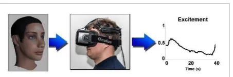
A virtual 3D face of woman was used as a stimulus for eliciting human reaction. Three types of 3D face fea-tures (distance-between-eyes, nose width and chin width) were used for human reaction elicitation and four EEG-based response signals (excitement, frus-tration, engagement/boredom and meditation) were observed and analyzed in previous research [46]. Anal-ysis of the results has shown that all three types of the 3D face feature have triggered similar human reaction signals, accordingly distance-between-eyes was select-ed and usselect-ed as a dynamic 3D face feature in further re-search [24], [26], [28]. From observed four EEG-based response signals, excitement is the most variable signal. A virtual 3D face of woman with changing dis-tance-between-eyes was used for input (control sig-nal) and EEG-based pre-processed excitement signal was measured as output (Figure 1) in this research. The output signal was recorded with Emotiv Epoc device. This device records EEG inputs from 14 chan-nels (in accordance with the international 10-20 loca-tions): AF3, F7, F3, FC5, T7, P7, O1, O2, P8, T8, FC6, F4, F8, AF4 [34]. Values of the excitement signal vary from 0 to 1. If excitement is low, the value is close to 0 and if it is high, the value is close to 1.
Figure 1
Input - Output Control Plant
etc.) [11], [39]. EEG-based emotion signals
(excitement, frustration, engagement/boredom and
meditation) are characterized as reliable and quick
response signals. Therefore, it is relevant to
construct and investigate methods and models of
recognition and estimation dependencies between
emotion signals and different stimuli and to design
the emotion feedback systems based on these
models [29], [31], [43].
Linear and nonlinear predictive models of the
input-output structure were proposed and
investigated for exploring dependencies of the
EEG-based emotion signals as a human response to
a dynamic virtual 3D face features when a virtual
3D face is observed without a virtual reality
headset [24], [26], [46]. The technique of dynamic
systems identification which ensures stability of the
models is applied to build these models [14].
Predictive models are necessary in the design of
predictor-based control systems [5], [6], [7], [15-17],
[37]. Predictor-based control principles were
applied to the control of human emotion signals
when a 3D face was observed without a virtual
reality headset [25], [27].
In this paper, three predictor-based control
schemes with a minimum variance or a generalized
minimum variance control quality, constrained
control signal magnitude and changing rate are
developed for the control of human excitement as
response to a dynamic 3D face when it is observed
using virtual reality headset. The first results of
experiments in this direction were published in
[28]. Different generalized minimum variance
control criterion is used in this paper. Stability and
systematic control error of the closed loop system
are investigated. Selection of the weight coefficient
of a generalized minimum variance criterion is
based on stability condition of closed loop system
and admissible value of systematic control error.
The technique of systems identification which
ensures stability and possible higher gain of the
predictive models of the control plant is applied.
Moreover, quantity of volunteers is expanded on
purpose to increase reliability of the experimental
control schemes comparison results.
2. Control Plant
A virtual 3D face of woman was used as a stimulus
for eliciting human reaction. Three types of 3D face
features (distance-between-eyes, nose width and
chin width) were used for human reaction
elicitation and four EEG-based response signals
(excitement, frustration, engagement/boredom and
meditation) were observed and analyzed in
previous research [46]. Analysis of the results
has shown that all three types of the 3D face
feature have triggered similar human reaction
signals, accordingly distance-between-eyes
was selected and used as a dynamic 3D face
feature in further research [24], [26], [28].
From observed four EEG-based response
signals, excitement is the most variable signal.
A virtual 3D face of woman with changing
distance-between-eyes was used for input
(control signal) and EEG-based pre-processed
excitement signal was measured as output
(Figure 1) in this research. The output signal
was recorded with
Emotiv Epoc
device. This
device records EEG inputs from 14 channels
(in accordance with the international 10-20
locations): AF3, F7, F3, FC5, T7, P7, O1, O2, P8,
T8, FC6, F4, F8, AF4 [34]. Values of the
excitement signal vary from 0 to 1. If
excitement is low, the value is close to 0 and if
it is high, the value is close to 1.
Figure 1. Input - Output Control Plant
Other 3D faces were formed by changing
distance-between-eyes in an extreme manner
(Figure 2).
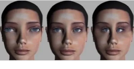
Figure 2. A virtual 3D face of the woman with changing (the smallest (right), normal (middle) and the largest (left)) distance-between-eyes
The transitions between normal and extreme
stages were programmed. “Neutral” face has
0 value, largest distance-between-eyes
corresponds to value 3 and smallest
distance-between-eyes corresponds to value -3. The
excitement and changing
distance-between-eyes signals were recorded with the sampling
period of
T
0=0.5
.
3. Model Building
Cross-correlation analysis demonstrated that
there is a relative high correlation between
observations of the EEG-based excitement
signal and changing distance-between-eyes in
virtual 3D face [28]. The shift of the maximum
Other 3D faces were formed by changing distance-be-tween-eyes in an extreme manner (Figure 2).
Information Technology and Control 2019/2/48 252
Figure 2
A virtual 3D face of the woman with changing (the smallest (right), normal (middle) and the largest (left)) distance-between-eyes
etc.) [11], [39]. EEG-based emotion signals
(excitement, frustration, engagement/boredom and
meditation) are characterized as reliable and quick
response signals. Therefore, it is relevant to
construct and investigate methods and models of
recognition and estimation dependencies between
emotion signals and different stimuli and to design
the emotion feedback systems based on these
models [29], [31], [43].
Linear and nonlinear predictive models of the
input-output structure were proposed and
investigated for exploring dependencies of the
EEG-based emotion signals as a human response to
a dynamic virtual 3D face features when a virtual
3D face is observed without a virtual reality
headset [24], [26], [46]. The technique of dynamic
systems identification which ensures stability of the
models is applied to build these models [14].
Predictive models are necessary in the design of
predictor-based control systems [5], [6], [7], [15-17],
[37]. Predictor-based control principles were
applied to the control of human emotion signals
when a 3D face was observed without a virtual
reality headset [25], [27].
In this paper, three predictor-based control
schemes with a minimum variance or a generalized
minimum variance control quality, constrained
control signal magnitude and changing rate are
developed for the control of human excitement as
response to a dynamic 3D face when it is observed
using virtual reality headset. The first results of
experiments in this direction were published in
[28]. Different generalized minimum variance
control criterion is used in this paper. Stability and
systematic control error of the closed loop system
are investigated. Selection of the weight coefficient
of a generalized minimum variance criterion is
based on stability condition of closed loop system
and admissible value of systematic control error.
The technique of systems identification which
ensures stability and possible higher gain of the
predictive models of the control plant is applied.
Moreover, quantity of volunteers is expanded on
purpose to increase reliability of the experimental
control schemes comparison results.
2. Control Plant
A virtual 3D face of woman was used as a stimulus
for eliciting human reaction. Three types of 3D face
features (distance-between-eyes, nose width and
chin width) were used for human reaction
elicitation and four EEG-based response signals
(excitement, frustration, engagement/boredom and
meditation) were observed and analyzed in
previous research [46]. Analysis of the results
has shown that all three types of the 3D face
feature have triggered similar human reaction
signals, accordingly distance-between-eyes
was selected and used as a dynamic 3D face
feature in further research [24], [26], [28].
From observed four EEG-based response
signals, excitement is the most variable signal.
A virtual 3D face of woman with changing
distance-between-eyes was used for input
(control signal) and EEG-based pre-processed
excitement signal was measured as output
(Figure 1) in this research. The output signal
was recorded with
Emotiv Epoc
device. This
device records EEG inputs from 14 channels
(in accordance with the international 10-20
locations): AF3, F7, F3, FC5, T7, P7, O1, O2, P8,
T8, FC6, F4, F8, AF4 [34]. Values of the
excitement signal vary from 0 to 1. If
excitement is low, the value is close to 0 and if
it is high, the value is close to 1.
Figure 1. Input - Output Control Plant
Other 3D faces were formed by changing
distance-between-eyes in an extreme manner
(Figure 2).
Figure 2. A virtual 3D face of the woman with changing
(the smallest (right), normal (middle) and the largest
(left)) distance-between-eyes
The transitions between normal and extreme
stages were programmed. “Neutral” face has
0 value, largest distance-between-eyes
corresponds to value 3 and smallest
distance-between-eyes corresponds to value -3. The
excitement and changing
distance-between-eyes signals were recorded with the sampling
period of
T
0=0.5
.
3. Model Building
Cross-correlation analysis demonstrated that
there is a relative high correlation between
observations of the EEG-based excitement
signal and changing distance-between-eyes in
virtual 3D face [28]. The shift of the maximum
3. Model Building
Cross-correlation analysis demonstrated that there is a relative high correlation between observations of the EEG-based excitement signal and changing dis-tance-between-eyes in virtual 3D face [28]. The shift of the maximum values of the cross-correlations in relation to the origin allows stating that there exist linear dynamic relations between input and output signals. Accordingly, dependency between human ex-citement as response to a virtual 3D face with chang-ing distance-between-eyes is described by a linear input-output structure model [24]
there is a relative high correlation between observations of the EEG-based excitement signal and changing distance-between-eyes in virtual 3D face [28]. The shift of the maximum values of the cross-correlations in relation to the origin allows stating that there exist linear dynamic relations between input and output signals. Accordingly, dependency between human excitement as response to a virtual 3D face with changing distance-between-eyes is described by a linear input-output structure model [24]
A(z-1)y
t=θ0+B(z-1)xt+εt, (1)
where
A(z-1) =1+�a iz-i, n
i=1
B(z-1) =�b
jz-j, m≤n m
j=0
,
(2)
yt is an output (excitement), xt is input
(distance-between-eyes) signals, respectively, observed as
yt=y(tT0), xt=x(tT0)
with a sampling period T0, εt denotes the equation
error of white-noise type, z-1 is the backward-shift
operator (z-1x
t=xt-1.) and θ0 is a constant value.
Model (1) with permanent component θ0>0, which
evaluates that excitement signal is positive, is different from ordinary linear dynamic model. Equation (1) can be expressed in the following form
yt=yt|t-1+εt, (3)
where
yt|t-1=θ0+z[1-A(z-1)]yt-1+B(z-1)xt (4)
is one-step-ahead output prediction model, z is a toward-shift operator (zyt=yt+1).
Parameters (coefficients bjand ai, degrees m and n
of the polynomials (2) and constant θ0) of the model
(1) are unknown. They must be estimated in the identification process, according to the observations obtained during the experiments with the volunteers.
Basic techniques of system identification and numerical schemes of computing the estimates [8], [9], [32], [40] do not ensure stability of the dynamic models. As a solution to this problem, the techniques and numerical methods of dynamic system identification were developed [14].
Applying this technique, the current estimates of the parameters are obtained from the condition
c
�t : Q�t(c) =
1
t-n � εk|k2 -1(c) t
k=n+1 (5)
→ min,
c ∈Ωc
where
cT=[θ
0,bo,b1,…,bm,a1,a2,…,an] (6)
is a vector of the coefficients of the polynomials (2) and parameter θ0,
εt+1|t(c) =yt+1-yt+1|t (7)
is one-step-ahead output prediction error,
Ωc=�ai: � ziA�<1, i=1, 2,…, n � (8)
is stability domain (unity disk) for the model (1), ziAare the roots of the polynomial
ziA: A(z) =0, i=1,….,n,
A(z) =znA(z-1) (9)
𝑇𝑇𝑇𝑇 is a vector transpose sign, sign || denotes the absolute value.
The numerical algorithms for computing the estimates as a solution of the minimization problem (5)-(9) were investigated in [24], [26], [28].
4.
Control with Constraints
Schemes
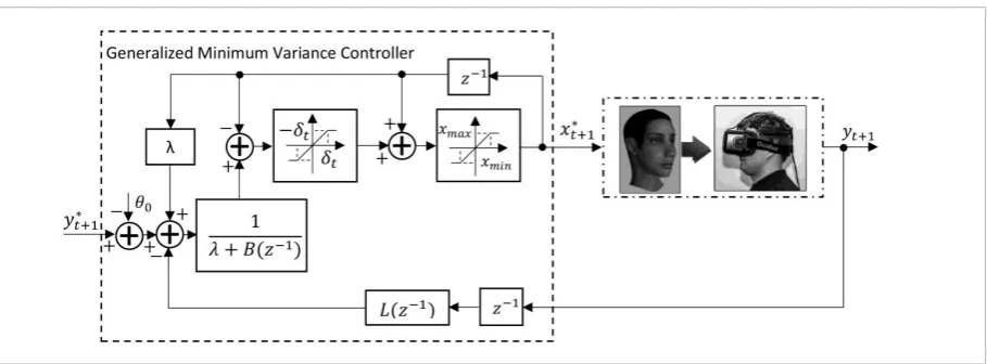
The control law synthesis for stochastic control plant (1) is often based on minimizing variance of the deviation between the observed output signal and the reference signal (minimum variance control) [1], [12], [41]. Generalized minimum variance control is obtained by introducing control costing [2], [4], [6, 7], [37], [42].
Basic techniques of a minimum variance or generalized minimum variance control are developed without evaluation of possible control signal constraints. Accordingly, techniques and schemes with constrained control signal magnitude and change rate for linear and nonlinear plants were constructed [15-23].
Applying this technique for the control plant (1), the control law is obtained from the condition
xt+1* : Qt(xt+1)→xmin
t+1∈Ωx, (10)
(1)
where
there is a relative high correlation between observations of the EEG-based excitement signal and changing distance-between-eyes in virtual 3D face [28]. The shift of the maximum values of the cross-correlations in relation to the origin allows stating that there exist linear dynamic relations between input and output signals. Accordingly, dependency between human excitement as response to a virtual 3D face with changing distance-between-eyes is described by a linear input-output structure model [24]
A(z-1)y
t=θ0+B(z-1)xt+εt, (1)
where
A(z-1) =1+�a iz-i, n
i=1
B(z-1) =�b
jz-j, m≤n m
j=0
,
(2)
yt is an output (excitement), xt is input
(distance-between-eyes) signals, respectively, observed as
yt=y(tT0), xt=x(tT0)
with a sampling period T0, εt denotes the equation
error of white-noise type, z-1 is the backward-shift
operator (z-1x
t=xt-1.) and θ0 is a constant value.
Model (1) with permanent component θ0>0, which
evaluates that excitement signal is positive, is different from ordinary linear dynamic model. Equation (1) can be expressed in the following form
yt=yt|t-1+εt, (3)
where
yt|t-1=θ0+z[1-A(z-1)]yt-1+B(z-1)xt (4)
is one-step-ahead output prediction model, z is a toward-shift operator (zyt=yt+1).
Parameters (coefficients bjand ai, degrees m and n
of the polynomials (2) and constant θ0) of the model
(1) are unknown. They must be estimated in the identification process, according to the observations obtained during the experiments with the volunteers.
Basic techniques of system identification and numerical schemes of computing the estimates [8], [9], [32], [40] do not ensure stability of the dynamic models. As a solution to this problem, the techniques and numerical methods of dynamic system identification were developed [14].
Applying this technique, the current estimates of the parameters are obtained from the condition
c
�t : Q�t(c) =
1
t-n � εk|k2 -1(c) t
k=n+1 (5)
→ min,
c ∈Ωc
where
cT=[θ
0,bo,b1,…,bm,a1,a2,…,an] (6)
is a vector of the coefficients of the polynomials (2) and parameter θ0,
εt+1|t(c) =yt+1-yt+1|t (7)
is one-step-ahead output prediction error, Ωc= �ai: � ziA� <1, i=1, 2,…, n � (8)
is stability domain (unity disk) for the model (1), ziAare the roots of the polynomial
ziA: A(z) =0, i=1,….,n,
A(z) =znA(z-1) (9) 𝑇𝑇𝑇𝑇 is a vector transpose sign, sign || denotes the absolute value.
The numerical algorithms for computing the estimates as a solution of the minimization problem (5)-(9) were investigated in [24], [26], [28].
4.
Control with Constraints
Schemes
The control law synthesis for stochastic control plant (1) is often based on minimizing variance of the deviation between the observed output signal and the reference signal (minimum variance control) [1], [12], [41]. Generalized minimum variance control is obtained by introducing control costing [2], [4], [6, 7], [37], [42].
Basic techniques of a minimum variance or generalized minimum variance control are developed without evaluation of possible control signal constraints. Accordingly, techniques and schemes with constrained control signal magnitude and change rate for linear and nonlinear plants were constructed [15-23].
Applying this technique for the control plant (1), the control law is obtained from the condition
xt+1* : Qt(xt+1)→xt+1∈Ωxmin , (10)
(2)
yt is an output (excitement), xt is input (distance-be-tween-eyes) signals, respectively, observed as
there is a relative high correlation between observations of the EEG-based excitement signal and changing distance-between-eyes in virtual 3D face [28]. The shift of the maximum values of the cross-correlations in relation to the origin allows stating that there exist linear dynamic relations between input and output signals. Accordingly, dependency between human excitement as response to a virtual 3D face with changing distance-between-eyes is described by a linear input-output structure model [24]
A(z-1)y
t= θ0+B(z-1)xt+εt, (1)
where
A(z-1) =1+�a iz-i, n
i=1
B(z-1) =�b
jz-j, m≤n m
j=0
,
(2)
yt is an output (excitement), xt is input
(distance-between-eyes) signals, respectively, observed as
yt=y(tT0), xt=x(tT0)
with a sampling period T0, εt denotes the equation
error of white-noise type, z-1 is the backward-shift
operator (z-1x
t=xt-1.) and θ0 is a constant value.
Model (1) with permanent component θ0>0, which
evaluates that excitement signal is positive, is different from ordinary linear dynamic model. Equation (1) can be expressed in the following form
yt=yt|t-1+ εt, (3)
where
yt|t-1= θ0+z[1-A(z-1)]yt-1+B(z-1)xt (4)
is one-step-ahead output prediction model, z is a toward-shift operator (zyt=yt+1).
Parameters (coefficients bjand ai, degrees m and n
of the polynomials (2) and constant θ0) of the model
(1) are unknown. They must be estimated in the identification process, according to the observations obtained during the experiments with the volunteers.
Basic techniques of system identification and numerical schemes of computing the estimates [8], [9], [32], [40] do not ensure stability of the dynamic models. As a solution to this problem, the techniques and numerical methods of dynamic system identification were developed [14].
Applying this technique, the current estimates of the parameters are obtained from the condition
c
�t : Q�t(c) =
1
t-n � εk|k2 -1(c) t
k=n+1 (5)
→ min,
c ∈Ωc
where
cT=[θ
0,bo,b1,…,bm,a1,a2,…,an] (6)
is a vector of the coefficients of the polynomials (2) and parameter θ0,
εt+1|t(c) =yt+1-yt+1|t (7)
is one-step-ahead output prediction error,
Ωc= �ai: � ziA� <1, i=1, 2,…, n � (8)
is stability domain (unity disk) for the model (1), ziAare the roots of the polynomial
ziA: A(z) =0, i=1,….,n,
A(z) =znA(z-1) (9) 𝑇𝑇𝑇𝑇 is a vector transpose sign, sign || denotes the absolute value.
The numerical algorithms for computing the estimates as a solution of the minimization problem (5)-(9) were investigated in [24], [26], [28].
4.
Control with Constraints
Schemes
The control law synthesis for stochastic control plant (1) is often based on minimizing variance of the deviation between the observed output signal and the reference signal (minimum variance control) [1], [12], [41]. Generalized minimum variance control is obtained by introducing control costing [2], [4], [6, 7], [37], [42].
Basic techniques of a minimum variance or generalized minimum variance control are developed without evaluation of possible control signal constraints. Accordingly, techniques and schemes with constrained control signal magnitude and change rate for linear and nonlinear plants were constructed [15-23].
Applying this technique for the control plant (1), the control law is obtained from the condition
xt+1* : Qt(xt+1)→xt+1∈Ωmin
x, (10)
with a sampling period T0, εt denotes the equation er-ror of white-noise type, z-1 is the backward-shift oper-ator (z-1 x
t = xt-1 ) and θ0 is a constant value.
Model (1) with permanent component θ0>0, which evaluates that excitement signal is positive, is differ-ent from ordinary linear dynamic model.
Equation (1) can be expressed in the following form
there is a relative high correlation between observations of the EEG-based excitement signal and changing distance-between-eyes in virtual 3D face [28]. The shift of the maximum values of the cross-correlations in relation to the origin allows stating that there exist linear dynamic relations between input and output signals. Accordingly, dependency between human excitement as response to a virtual 3D face with changing distance-between-eyes is described by a linear input-output structure model [24]
A(z-1)y
t= θ0+B(z-1)xt+εt, (1)
where
A(z-1) =1+�a iz-i, n
i=1
B(z-1) =�b
jz-j, m≤n m
j=0
,
(2)
yt is an output (excitement), xt is input
(distance-between-eyes) signals, respectively, observed as
yt=y(tT0), xt=x(tT0)
with a sampling period T0, εt denotes the equation
error of white-noise type, z-1 is the backward-shift
operator (z-1x
t=xt-1.) and θ0 is a constant value.
Model (1) with permanent component θ0>0, which
evaluates that excitement signal is positive, is different from ordinary linear dynamic model. Equation (1) can be expressed in the following form
yt=yt|t-1+ εt, (3)
where
yt|t-1= θ0+z[1-A(z-1)]yt-1+B(z-1)xt (4)
is one-step-ahead output prediction model, z is a toward-shift operator (zyt=yt+1).
Parameters (coefficients bjand ai, degrees m and n
of the polynomials (2) and constant θ0) of the model
(1) are unknown. They must be estimated in the identification process, according to the observations obtained during the experiments with the volunteers.
Basic techniques of system identification and numerical schemes of computing the estimates [8], [9], [32], [40] do not ensure stability of the dynamic models. As a solution to this problem, the techniques and numerical methods of dynamic system identification were developed [14].
Applying this technique, the current estimates of the parameters are obtained from the condition
c
�t : Q�t(c) =
1
t-n � εk|k2 -1(c) t
k=n+1 (5)
→ min,
c ∈Ωc
where
cT=[θ
0,bo,b1,…,bm,a1,a2,…,an] (6)
is a vector of the coefficients of the polynomials (2) and parameter θ0,
εt+1|t(c) =yt+1-yt+1|t (7)
is one-step-ahead output prediction error,
Ωc= �ai: � ziA� <1, i=1, 2,…, n � (8)
is stability domain (unity disk) for the model (1), ziAare the roots of the polynomial
ziA: A(z) =0, i=1,….,n,
A(z) =znA(z-1) (9) 𝑇𝑇𝑇𝑇 is a vector transpose sign, sign || denotes the absolute value.
The numerical algorithms for computing the estimates as a solution of the minimization problem (5)-(9) were investigated in [24], [26], [28].
4.
Control with Constraints
Schemes
The control law synthesis for stochastic control plant (1) is often based on minimizing variance of the deviation between the observed output signal and the reference signal (minimum variance control) [1], [12], [41]. Generalized minimum variance control is obtained by introducing control costing [2], [4], [6, 7], [37], [42].
Basic techniques of a minimum variance or generalized minimum variance control are developed without evaluation of possible control signal constraints. Accordingly, techniques and schemes with constrained control signal magnitude and change rate for linear and nonlinear plants were constructed [15-23].
Applying this technique for the control plant (1), the control law is obtained from the condition
xt+1* : Qt(xt+1)→xt+1∈minΩ
x, (10)
(3)
where
there is a relative high correlation between observations of the EEG-based excitement signal and changing distance-between-eyes in virtual 3D face [28]. The shift of the maximum values of the cross-correlations in relation to the origin allows stating that there exist linear dynamic relations between input and output signals. Accordingly, dependency between human excitement as response to a virtual 3D face with changing distance-between-eyes is described by a linear input-output structure model [24]
A(z-1)y
t= θ0+B(z-1)xt+εt, (1)
where
A(z-1) =1+�a iz-i, n
i=1
B(z-1) =�b
jz-j, m ≤ n m
j=0
,
(2)
yt is an output (excitement), xt is input
(distance-between-eyes) signals, respectively, observed as
yt=y(tT0), xt=x(tT0)
with a sampling period T0, εt denotes the equation
error of white-noise type, z-1 is the backward-shift
operator (z-1x
t=xt-1.) and θ0 is a constant value.
Model (1) with permanent component θ0>0, which
evaluates that excitement signal is positive, is different from ordinary linear dynamic model. Equation (1) can be expressed in the following form
yt=yt|t-1+εt, (3)
where
yt|t-1= θ0+z[1-A(z-1)]yt-1+B(z-1)xt (4)
is one-step-ahead output prediction model, z is a toward-shift operator (zyt=yt+1).
Parameters (coefficients bjand ai, degrees m and n
of the polynomials (2) and constant θ0) of the model
(1) are unknown. They must be estimated in the identification process, according to the observations obtained during the experiments with the volunteers.
Basic techniques of system identification and numerical schemes of computing the estimates [8], [9], [32], [40] do not ensure stability of the dynamic models. As a solution to this problem, the techniques and numerical methods of dynamic system identification were developed [14].
Applying this technique, the current estimates of the parameters are obtained from the condition
c
�t : Q�t(c) =
1
t-n � εk|k2 -1(c) t
k=n+1 (5)
→ min,
c ∈Ωc
where
cT=[θ
0,bo,b1,…,bm,a1,a2,…,an] (6)
is a vector of the coefficients of the polynomials (2) and parameter θ0,
εt+1|t(c) =yt+1-yt+1|t (7)
is one-step-ahead output prediction error,
Ωc=�ai: � ziA�<1, i=1, 2,…, n � (8)
is stability domain (unity disk) for the model (1), ziAare the roots of the polynomial
ziA: A(z) =0, i=1,….,n,
A(z) =znA(z-1) (9)
𝑇𝑇𝑇𝑇 is a vector transpose sign, sign || denotes the absolute value.
The numerical algorithms for computing the estimates as a solution of the minimization problem (5)-(9) were investigated in [24], [26], [28].
4.
Control with Constraints
Schemes
The control law synthesis for stochastic control plant (1) is often based on minimizing variance of the deviation between the observed output signal and the reference signal (minimum variance control) [1], [12], [41]. Generalized minimum variance control is obtained by introducing control costing [2], [4], [6, 7], [37], [42].
Basic techniques of a minimum variance or generalized minimum variance control are developed without evaluation of possible control signal constraints. Accordingly, techniques and schemes with constrained control signal magnitude and change rate for linear and nonlinear plants were constructed [15-23].
Applying this technique for the control plant (1), the control law is obtained from the condition
xt+1* : Qt(xt+1)→xmin
t+1∈Ωx, (10)
(4)
is one-step-ahead output prediction model, z is a to-ward-shift operator (zyt = yt+1).
Parameters (coefficients bj and ai, degrees m and n of
the polynomials (2) and constant θ0) of the model (1)
are unknown. They must be estimated in the identi-fication process, according to the observations ob-tained during the experiments with the volunteers. Basic techniques of system identification and numer-ical schemes of computing the estimates [8], [9], [32], [40] do not ensure stability of the dynamic models. As a solution to this problem, the techniques and numer-ical methods of dynamic system identification were developed [14].
Applying this technique, the current estimates of the parameters are obtained from the condition
there is a relative high correlation between observations of the EEG-based excitement signal and changing distance-between-eyes in virtual 3D face [28]. The shift of the maximum values of the cross-correlations in relation to the origin allows stating that there exist linear dynamic relations between input and output signals. Accordingly, dependency between human excitement as response to a virtual 3D face with changing distance-between-eyes is described by a linear input-output structure model [24]
A(z-1)y
t= θ0+B(z-1)xt+εt, (1)
where
A(z-1) =1+�a iz-i, n
i=1
B(z-1) =�b
jz-j, m≤n m
j=0
,
(2)
yt is an output (excitement), xt is input
(distance-between-eyes) signals, respectively, observed as
yt=y(tT0), xt=x(tT0)
with a sampling period T0, εt denotes the equation
error of white-noise type, z-1 is the backward-shift
operator (z-1x
t=xt-1.) and θ0 is a constant value.
Model (1) with permanent component θ0>0, which
evaluates that excitement signal is positive, is different from ordinary linear dynamic model. Equation (1) can be expressed in the following form
yt=yt|t-1+ εt, (3)
where
yt|t-1= θ0+z[1-A(z-1)]yt-1+B(z-1)xt (4)
is one-step-ahead output prediction model, z is a toward-shift operator (zyt=yt+1).
Parameters (coefficients bjand ai, degrees m and n
of the polynomials (2) and constant θ0) of the model
(1) are unknown. They must be estimated in the identification process, according to the observations obtained during the experiments with the volunteers.
Basic techniques of system identification and numerical schemes of computing the estimates [8], [9], [32], [40] do not ensure stability of the dynamic models. As a solution to this problem, the techniques and numerical methods of dynamic system identification were developed [14].
Applying this technique, the current estimates of the parameters are obtained from the condition
c�t : Q�t(c) =
1
t-n � εk|k2 -1(c) t
k=n+1 (5)
→ min,
c ∈Ωc
where
cT=[θ
0,bo,b1,…,bm,a1,a2,…,an] (6)
is a vector of the coefficients of the polynomials (2) and parameter θ0,
εt+1|t(c) =yt+1-yt+1|t (7)
is one-step-ahead output prediction error,
Ωc= �ai: � ziA� <1, i=1, 2,…, n � (8)
is stability domain (unity disk) for the model (1), ziAare the roots of the polynomial
ziA: A(z) =0, i=1,….,n,
A(z) =znA(z-1) (9) 𝑇𝑇𝑇𝑇 is a vector transpose sign, sign || denotes the absolute value.
The numerical algorithms for computing the estimates as a solution of the minimization problem (5)-(9) were investigated in [24], [26], [28].
4.
Control with Constraints
Schemes
The control law synthesis for stochastic control plant (1) is often based on minimizing variance of the deviation between the observed output signal and the reference signal (minimum variance control) [1], [12], [41]. Generalized minimum variance control is obtained by introducing control costing [2], [4], [6, 7], [37], [42].
Basic techniques of a minimum variance or generalized minimum variance control are developed without evaluation of possible control signal constraints. Accordingly, techniques and schemes with constrained control signal magnitude and change rate for linear and nonlinear plants were constructed [15-23].
Applying this technique for the control plant (1), the control law is obtained from the condition
xt+1* : Qt(xt+1)→xt+1∈Ωmin
x, (10)
(5)
where
there is a relative high correlation between observations of the EEG-based excitement signal and changing distance-between-eyes in virtual 3D face [28]. The shift of the maximum values of the cross-correlations in relation to the origin allows stating that there exist linear dynamic relations between input and output signals. Accordingly, dependency between human excitement as response to a virtual 3D face with changing distance-between-eyes is described by a linear input-output structure model [24]
A(z-1)y
t=θ0+B(z-1)xt+εt, (1)
where
A(z-1) =1+�a iz-i, n
i=1
B(z-1) =�b
jz-j, m≤n m
j=0
,
(2)
yt is an output (excitement), xt is input
(distance-between-eyes) signals, respectively, observed as
yt=y(tT0), xt=x(tT0)
with a sampling period T0, εt denotes the equation
error of white-noise type, z-1 is the backward-shift
operator (z-1x
t=xt-1.) and θ0 is a constant value.
Model (1) with permanent component θ0>0, which
evaluates that excitement signal is positive, is different from ordinary linear dynamic model. Equation (1) can be expressed in the following form
yt=yt|t-1+ εt, (3)
where
yt|t-1=θ0+z[1-A(z-1)]yt-1+B(z-1)xt (4)
is one-step-ahead output prediction model, z is a toward-shift operator (zyt=yt+1).
Parameters (coefficients bjand ai, degrees m and n
of the polynomials (2) and constant θ0) of the model
(1) are unknown. They must be estimated in the identification process, according to the observations obtained during the experiments with the volunteers.
Basic techniques of system identification and numerical schemes of computing the estimates [8], [9], [32], [40] do not ensure stability of the dynamic models. As a solution to this problem, the techniques and numerical methods of dynamic system identification were developed [14].
Applying this technique, the current estimates of the parameters are obtained from the condition
c
�t : Q�t(c) =
1
t-n � εk|k2 -1(c) t
k=n+1 (5)
→ min,
c ∈Ωc
where
cT=[θ
0,bo,b1,…,bm,a1,a2,…,an] (6)
is a vector of the coefficients of the polynomials (2) and parameter θ0,
εt+1|t(c) =yt+1-yt+1|t (7)
is one-step-ahead output prediction error,
Ωc= �ai: � ziA� <1, i=1, 2,…, n � (8)
is stability domain (unity disk) for the model (1), ziAare the roots of the polynomial
ziA: A(z) =0, i=1,….,n,
A(z) =znA(z-1) (9) 𝑇𝑇𝑇𝑇 is a vector transpose sign, sign || denotes the absolute value.
The numerical algorithms for computing the estimates as a solution of the minimization problem (5)-(9) were investigated in [24], [26], [28].
4.
Control with Constraints
Schemes
The control law synthesis for stochastic control plant (1) is often based on minimizing variance of the deviation between the observed output signal and the reference signal (minimum variance control) [1], [12], [41]. Generalized minimum variance control is obtained by introducing control costing [2], [4], [6, 7], [37], [42].
Basic techniques of a minimum variance or generalized minimum variance control are developed without evaluation of possible control signal constraints. Accordingly, techniques and schemes with constrained control signal magnitude and change rate for linear and nonlinear plants were constructed [15-23].
Applying this technique for the control plant (1), the control law is obtained from the condition
xt+1* : Qt(xt+1)→xt+1∈Ωmin
x, (10)
(6)
is a vector of the coefficients of the polynomials (2) and parameter θ0,
there is a relative high correlation between observations of the EEG-based excitement signal and changing distance-between-eyes in virtual 3D face [28]. The shift of the maximum values of the cross-correlations in relation to the origin allows stating that there exist linear dynamic relations between input and output signals. Accordingly, dependency between human excitement as response to a virtual 3D face with changing distance-between-eyes is described by a linear input-output structure model [24]
A(z-1)y
t=θ0+B(z-1)xt+εt, (1)
where
A(z-1) =1+�a iz-i, n
i=1
B(z-1) =�b
jz-j, m ≤ n m
j=0
,
(2)
yt is an output (excitement), xt is input
(distance-between-eyes) signals, respectively, observed as
yt=y(tT0), xt=x(tT0)
with a sampling period T0, εt denotes the equation
error of white-noise type, z-1 is the backward-shift
operator (z-1x
t=xt-1.) and θ0 is a constant value.
Model (1) with permanent component θ0>0, which
evaluates that excitement signal is positive, is different from ordinary linear dynamic model. Equation (1) can be expressed in the following form
yt=yt|t-1+ εt, (3)
where
yt|t-1=θ0+z[1-A(z-1)]yt-1+B(z-1)xt (4)
is one-step-ahead output prediction model, z is a toward-shift operator (zyt=yt+1).
Parameters (coefficients bjand ai, degrees m and n
of the polynomials (2) and constant θ0) of the model
(1) are unknown. They must be estimated in the identification process, according to the observations obtained during the experiments with the volunteers.
Basic techniques of system identification and numerical schemes of computing the estimates [8], [9], [32], [40] do not ensure stability of the dynamic models. As a solution to this problem, the techniques and numerical methods of dynamic system identification were developed [14].
Applying this technique, the current estimates of the parameters are obtained from the condition
c
�t : Q�t(c) =
1
t-n � εk|k2 -1(c) t
k=n+1 (5)
→ min,
c ∈Ωc
where
cT=[θ
0,bo,b1,…,bm,a1,a2,…,an] (6)
is a vector of the coefficients of the polynomials (2) and parameter θ0,
εt+1|t(c) =yt+1-yt+1|t (7)
is one-step-ahead output prediction error,
Ωc= �ai: � ziA� <1, i=1, 2,…, n � (8)
is stability domain (unity disk) for the model (1), ziAare the roots of the polynomial
ziA: A(z) =0, i=1,….,n,
A(z) =znA(z-1) (9) 𝑇𝑇𝑇𝑇 is a vector transpose sign, sign || denotes the absolute value.
The numerical algorithms for computing the estimates as a solution of the minimization problem (5)-(9) were investigated in [24], [26], [28].
4.
Control with Constraints
Schemes
The control law synthesis for stochastic control plant (1) is often based on minimizing variance of the deviation between the observed output signal and the reference signal (minimum variance control) [1], [12], [41]. Generalized minimum variance control is obtained by introducing control costing [2], [4], [6, 7], [37], [42].
Basic techniques of a minimum variance or generalized minimum variance control are developed without evaluation of possible control signal constraints. Accordingly, techniques and schemes with constrained control signal magnitude and change rate for linear and nonlinear plants were constructed [15-23].
Applying this technique for the control plant (1), the control law is obtained from the condition
xt+1* : Qt(xt+1)→xt+1∈minΩx, (10)
(7)
is one-step-ahead output prediction error,
there is a relative high correlation between observations of the EEG-based excitement signal and changing distance-between-eyes in virtual 3D face [28]. The shift of the maximum values of the cross-correlations in relation to the origin allows stating that there exist linear dynamic relations between input and output signals. Accordingly, dependency between human excitement as response to a virtual 3D face with changing distance-between-eyes is described by a linear input-output structure model [24]
A(z-1)y
t=θ0+B(z-1)xt+εt, (1)
where
A(z-1) =1+�a iz-i, n
i=1
B(z-1) =�b
jz-j, m≤n m
j=0
,
(2)
yt is an output (excitement), xt is input
(distance-between-eyes) signals, respectively, observed as
yt=y(tT0), xt=x(tT0)
with a sampling period T0, εt denotes the equation
error of white-noise type, z-1 is the backward-shift
operator (z-1x
t=xt-1.) and θ0 is a constant value.
Model (1) with permanent component θ0>0, which
evaluates that excitement signal is positive, is different from ordinary linear dynamic model. Equation (1) can be expressed in the following form
yt=yt|t-1+εt, (3)
where
yt|t-1=θ0+z[1-A(z-1)]yt-1+B(z-1)xt (4)
is one-step-ahead output prediction model, z is a toward-shift operator (zyt=yt+1).
Parameters (coefficients bjand ai, degrees m and n
of the polynomials (2) and constant θ0) of the model
(1) are unknown. They must be estimated in the identification process, according to the observations obtained during the experiments with the volunteers.
Basic techniques of system identification and numerical schemes of computing the estimates [8], [9], [32], [40] do not ensure stability of the dynamic models. As a solution to this problem, the techniques and numerical methods of dynamic system identification were developed [14].
Applying this technique, the current estimates of the parameters are obtained from the condition
c
�t : Q�t(c) =
1
t-n � εk|k2 -1(c) t
k=n+1 (5)
→ min,
c ∈Ωc
where
cT=[θ
0,bo,b1,…,bm,a1,a2,…,an] (6)
is a vector of the coefficients of the polynomials (2) and parameter θ0,
εt+1|t(c) =yt+1-yt+1|t (7)
is one-step-ahead output prediction error, Ωc=�ai: � ziA�<1, i=1, 2,…, n � (8)
is stability domain (unity disk) for the model (1), ziAare the roots of the polynomial
ziA: A(z) =0, i=1,….,n,
A(z) =znA(z-1) (9) 𝑇𝑇𝑇𝑇 is a vector transpose sign, sign || denotes the absolute value.
The numerical algorithms for computing the estimates as a solution of the minimization problem (5)-(9) were investigated in [24], [26], [28].
4.
Control with Constraints
Schemes
The control law synthesis for stochastic control plant (1) is often based on minimizing variance of the deviation between the observed output signal and the reference signal (minimum variance control) [1], [12], [41]. Generalized minimum variance control is obtained by introducing control costing [2], [4], [6, 7], [37], [42].
Basic techniques of a minimum variance or generalized minimum variance control are developed without evaluation of possible control signal constraints. Accordingly, techniques and schemes with constrained control signal magnitude and change rate for linear and nonlinear plants were constructed [15-23].
Applying this technique for the control plant (1), the control law is obtained from the condition
xt+1* : Q
t(xt+1)→xmin
t+1∈Ωx, (10)
(8)
is stability domain (unity disk) for the model (1), zAi are the roots of the polynomial
there is a relative high correlation between observations of the EEG-based excitement signal and changing distance-between-eyes in virtual 3D face [28]. The shift of the maximum values of the cross-correlations in relation to the origin allows stating that there exist linear dynamic relations between input and output signals. Accordingly, dependency between human excitement as response to a virtual 3D face with changing distance-between-eyes is described by a linear input-output structure model [24]
A(z-1)y
t=θ0+B(z-1)xt+εt, (1)
where
A(z-1) =1+�a iz-i, n
i=1
B(z-1) =�b
jz-j, m≤n m
j=0
,
(2)
yt is an output (excitement), xt is input
(distance-between-eyes) signals, respectively, observed as
yt=y(tT0), xt=x(tT0)
with a sampling period T0, εt denotes the equation
error of white-noise type, z-1 is the backward-shift
operator (z-1x
t=xt-1.) and θ0 is a constant value.
Model (1) with permanent component θ0>0, which
evaluates that excitement signal is positive, is different from ordinary linear dynamic model. Equation (1) can be expressed in the following form
yt=yt|t-1+εt, (3)
where
yt|t-1=θ0+z[1-A(z-1)]yt-1+B(z-1)xt (4)
is one-step-ahead output prediction model, z is a toward-shift operator (zyt=yt+1).
Parameters (coefficients bjand ai, degrees m and n
of the polynomials (2) and constant θ0) of the model
(1) are unknown. They must be estimated in the identification process, according to the observations obtained during the experiments with the volunteers.
Basic techniques of system identification and numerical schemes of computing the estimates [8], [9], [32], [40] do not ensure stability of the dynamic models. As a solution to this problem, the techniques and numerical methods of dynamic system identification were developed [14].
Applying this technique, the current estimates of the parameters are obtained from the condition
c�t : Q�t(c) =
1
t-n � εk|k2 -1(c) t
k=n+1 (5)
→ min,
c ∈Ωc
where
cT=[θ
0,bo,b1,…,bm,a1,a2,…,an] (6)
is a vector of the coefficients of the polynomials (2) and parameter θ0,
εt+1|t(c) =yt+1-yt+1|t (7)
is one-step-ahead output prediction error,
Ωc=�ai: � ziA�<1, i=1, 2,…, n � (8)
is stability domain (unity disk) for the model (1), ziAare the roots of the polynomial
ziA: A(z) =0, i=1,….,n,
A(z) =znA(z-1) (9)
𝑇𝑇𝑇𝑇 is a vector transpose sign, sign || denotes the absolute value.
The numerical algorithms for computing the estimates as a solution of the minimization problem (5)-(9) were investigated in [24], [26], [28].
4.
Control with Constraints
Schemes
The control law synthesis for stochastic control plant (1) is often based on minimizing variance of the deviation between the observed output signal and the reference signal (minimum variance control) [1], [12], [41]. Generalized minimum variance control is obtained by introducing control costing [2], [4], [6, 7], [37], [42].
Basic techniques of a minimum variance or generalized minimum variance control are developed without evaluation of possible control signal constraints. Accordingly, techniques and schemes with constrained control signal magnitude and change rate for linear and nonlinear plants were constructed [15-23].
Applying this technique for the control plant (1), the control law is obtained from the condition
xt+1* : Qt(xt+1)→xt+1∈minΩ
x, (10)
(9)