https://doi.org/10.5194/angeo-37-561-2019 © Author(s) 2019. This work is distributed under the Creative Commons Attribution 4.0 License.
GUMICS-4 analysis of interplanetary coronal mass ejection impact
on Earth during low and typical Mach number solar winds
Antti Lakka1, Tuija I. Pulkkinen1,6, Andrew P. Dimmock2, Emilia Kilpua3, Matti Ala-Lahti3, Ilja Honkonen4, Minna Palmroth3, and Osku Raukunen5
1Department of Electronics and Nanoengineering, Aalto University, Espoo, Finland 2Swedish Institute of Space Physics, Uppsala, Sweden
3Department of Physics, University of Helsinki, Helsinki, Finland 4Finnish Meteorological Institute, Helsinki, Finland
5Department of Physics and Astronomy, University of Turku, Turku, Finland
6Department of Climate and Space Sciences and Engineering, University of Michigan, Ann Arbor, USA Correspondence:Antti Lakka ([email protected])
Received: 5 July 2018 – Discussion started: 13 July 2018
Revised: 17 June 2019 – Accepted: 19 June 2019 – Published: 11 July 2019
Abstract. We study the response of the Earth’s magneto-sphere to fluctuating solar wind conditions during interplane-tary coronal mass ejections (ICMEs) using the Grand Unified Magnetosphere-Ionosphere Coupling Simulation (GUMICS-4). The two ICME events occurred on 15–16 July 2012 and 29–30 April 2014. During the strong 2012 event, the so-lar wind upstream values reached up to 35 particles cm−3, speeds of up to 694 km s−1, and an interplanetary magnetic field of up to 22 nT, giving a Mach number of 2.3. The 2014 event was a moderate one, with the corresponding upstream values of 30 particles cm−3, 320 km s−1and 10 nT, indicating a Mach number of 5.8. We examine how the Earth’s space en-vironment dynamics evolves during both ICME events from both global and local perspectives, using well-established empirical models and in situ measurements as references. We show that on the large scale, and during moderate driv-ing, the GUMICS-4 results are in good agreement with the reference values. However, the local values, especially dur-ing high drivdur-ing, show more variation: such extreme condi-tions do not reproduce local measurements made deep in-side the magnetosphere. The same appeared to be true when the event was run with another global simulation. The cross-polar cap potential (CPCP) saturation is shown to depend on the Alfvén–Mach number of the upstream solar wind. How-ever, care must be taken in interpreting these results, as the CPCP is also sensitive to the simulation resolution.
1 Introduction
of the magnetic field (Burlaga et al., 1981). While there have been attempts to form a universal set of signatures to describe ICMEs (Gosling, 1990; Richardson and Cane, 2003), they vary significantly such that no single set of criteria is able to describe all the ICME events, and none of them is unique to ICMEs. For example, only one-third to one-half of all the ICMEs have a magnetic flux rope (or a magnetic cloud) (e.g., Gosling, 1990; Richardson and Cane, 2003), whose signa-tures combine enhanced magnetic field, reduced proton tem-perature, and the smooth rotation of the magnetic field over an interval of a day (Burlaga et al., 1981). While magnetic clouds are the most studied part of ICMEs due to their signif-icant potential to cause large space storms, their relationship with the entire ICME sequence still poses many questions (e.g., Kilpua et al., 2013). Moreover, if the ICME is suffi-ciently faster than the ambient solar wind plasma, a shock is formed ahead of the ICME (Goldstein et al., 1998), with a region of compressed solar wind plasma between the leading shock front and the magnetic cloud, referred to as the sheath region.
The sheath and ejecta are the most distinctive parts of ICMEs (see, e.g., Kilpua et al., 2017b), and both can drive in-tense magnetic storms (e.g., Tsurutani et al., 1988; Huttunen and Koskinen, 2004). However, they have clear differences in their solar wind conditions and, consequently, their cou-pling to the magnetosphere is different (Jianpeng et al., 2010; Pulkkinen et al., 2007; Kilpua et al., 2017b). ICME sheaths typically include high solar wind dynamic pressure and fluc-tuating IMF, including both northward and southward orien-tations within a short time period (Kilpua et al., 2017b). The duration of the sheath is also typically shorter than the fol-lowing cloud: for example. Zhang et al. (2012) obtained the average values of 10.6 and 30.6 h for sheaths and clouds, re-spectively. Sheaths are known to enhance high-latitude iono-spheric currents (Huttunen and Koskinen, 2004) and they are found to have higher coupling efficiency than clouds (Yermo-laev et al., 2012). The clouds typically enhance the equatorial ring current (Huttunen and Koskinen, 2004).
Due to the potential for strongly southward IMF orienta-tion, ICME magnetic clouds drive enhanced magnetospheric activity. Moreover, during cloud events, due to the combina-tion of generally high magnetic fields and low plasma den-sities, the solar wind Alfvén–Mach number MA can reach quite low values and even be close to unity. The role ofMA in solar wind–magnetosphere coupling has been highlighted in recent studies (Lavraud and Borovsky, 2008; Lopez et al., 2010; Myllys et al., 2016, 2017). In particular, the role of low
MAconditions typical for ICME magnetic cloud in the satu-ration of the ionospheric cross-polar cap potential (CPCP) has been a subject of several studies (e.g., Ridley, 2005, 2007; Lopez et al., 2010; Wilder et al., 2015; Myllys et al., 2016; Lakka et al., 2018).
Global MHD models have been used to study the ef-fects of ICMEs on the magnetospheric and ionospheric dy-namics. Wu et al. (2015) used the H3DMHD model (e.g.,
Wu et al., 2007) to examine a CME event on 15 March 2013. They found that the high-energy solar energetic proton time– intensity profile can be explained by the interaction of a CME-driven shock with the heliospheric current sheet em-bedded within nonuniform solar wind. A recent paper by Kubota et al. (2017) studied the Bastille Day geomagnetic storm event (15 July 2000) driven by a halo CME. They found that the inclusion of auroral conductivity in the iono-spheric part of the global MHD model by Tanaka (1994) led to saturation of the CPCP without any effect on the field-aligned currents, thus suggesting a current system with a dy-namo in the magnetosphere and a load in the ionosphere. The difficulty in assessing these studies is that they often do not include uncertainty estimate of the model results, while the methods are different for each study. Moreover, while the dif-ferent MHD simulations are based on the same plasma the-ory, the approaches are different in terms of the exact form of the equations, the numerical solutions, and the initial and boundary conditions, thus making comparisons of different models difficult. Nonetheless, understanding of the perfor-mance limits of the simulations is essential for meaningful comparisons to in situ measurements.
Regardless of the different approaches used in global codes, the performances of the models have been assessed in several studies. Usually such assessments are done through comparisons of the simulation results with in situ or remote observations of dynamic events or plasma processes (Birn et al., 2001; Pulkkinen et al., 2011; Honkonen et al., 2013). This is often not easy, as even small errors in the simulation configuration may create large differences with respect to the observations locally at a single point (Lakka et al., 2017), even if the simulation would reproduce the large-scale dy-namic sequence correctly. Moreover, recent studies (Juusola et al., 2014; Gordeev et al., 2015) have shown that none of the codes emerges as clearly superior to the others, each hav-ing their strengths and weaknesses. In the absence of uniform code performance testing methodology, validating the results individually is important.
lo-cation), the epsilon parameter (energy transferred through the magnetopause), the polar cap index (PCI) (CPCP), and in situ measurements by the Geotail and Cluster spacecraft (magnetic field magnitude). Both uncertainty estimate meth-ods are assessed and they are used if the method is valid for the chosen quantity.
This paper is structured in a following way: Sect. 2 de-scribes GUMICS-4 global MHD code and the simulation setup, Sect. 3 describes characteristics of the two ICME events and the executed simulations, Sect. 4 presents the main results and Sect. 5 includes the discussion followed by conclusions.
2 Methodology
2.1 GUMICS-4 global MHD simulation
The simulations were executed using the fourth edition of the Grand-Unified Magnetosphere-Ionosphere Coupling Simu-lation (GUMICS-4), in which a 3-D MHD magnetosphere is coupled with a spherical electrostatic ionosphere (Janhunen et al., 2012). The finite-volume MHD solver solves the ideal MHD equations with the separation of the magnetic field to a curl-free (dipole) component and divergent-free component created by currents external to the Earth (B=B0+B1(t )) (Tanaka, 1994). The MHD simulation box has dimensions of 32. . .−224RE in theXGSE direction and−64. . .+64REin both theYGSE andZGSE directions, while the inner bound-ary is spherical with a radius of 3.7RE. GUMICS-4 uses temporal subcycling and adaptive cartesian octogrid to im-prove temporal and spatial resolution in key regions, which means that it only runs on a single processor due to diffi-culties in parallelizing computations with two adaptive grids. The temporal subcycling reduces the number of MHD com-putations an order of magnitude while maintaining the local Courant–Friedrichs–Levy (CFL) constraint (Lions and Ciar-let, 2000, pp. 121–151). The adaptive grid ensures that when-ever there are large gradients, the grid is refined, thus resolv-ing smaller-scale features especially close to boundaries and current sheets.
The ionospheric grid is triangular and densest in the auro-ral oval, while in the polar caps the grid is still rather dense, with about 180 and 360 km spacing used in the two regions, respectively. The ionosphere is driven by field-aligned cur-rents and electron precipitation from the magnetosphere as well as by solar EUV ionization. Field-aligned currents con-tribute to the cross-polar cap potential through
∇ ·J= ∇ ·[6·(−∇φ+Vn×B)]= −j||
ˆ
b· ˆr, (1) where J is current density, 6 is the height-integrated con-ductivity tensor, φ is the ionospheric potential, Vn is the neutral wind caused by the Earth’s rotation,j|| is the field-aligned current, and (bˆ· ˆr) is the cosine of the angle be-tween the magnetic field directionbˆand the radial direction
ˆ
r (Janhunen et al., 2012). Electron precipitation and solar EUV ionization have contributions to the height-integrated Pedersen and Hall conductivities with solar EUV ionization parametrized by the 10.7 cm solar radio flux that has a numer-ical value of 100×10−22W m−2. Electron precipitation af-fects the altitude-resolved ionospheric electron densities and are used when computing the height-integrated Pedersen and Hall conductivities. The details on the ionospheric part of GUMICS-4 can be found in Janhunen and Huuskonen (1993) and Janhunen (1996).
The region between the MHD magnetosphere and the elec-trostatic spherical ionosphere is a passive medium where no currents flow perpendicularly to the magnetic field. The mag-netosphere is coupled to the ionosphere using dipole map-ping of the field-aligned current pattern and the electron pre-cipitation from the magnetosphere to the ionosphere and the electric potential from the ionosphere to the magnetosphere. This feedback loop is updated every 4 s.
2.2 GUMICS simulations of two ICME events
We use both 0.5 and 0.25RE maximum spatial resolutions as well as varying dipole tilt angles in this study. Two com-plete ICME periods were simulated using 0.5REresolution by starting with nominal solar wind conditions preceding the events and ending with nominal conditions following the events. To give the GUMICS-4 magnetosphere time to form (Lakka et al., 2017), the simulations were initialized with 2 h of constant solar wind driving using upstream values equal to those during the first minute of the actual simulation (n,|V|,|B|values of 4 cm−3, 310 km s−1and 1.1 nT for the 2012 event, and 11 cm−3, 300 km s−1and 1.8 nT for the 2014 event).
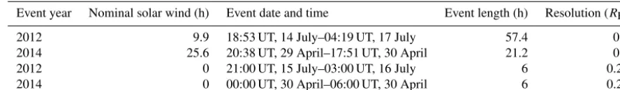
Due to computational limitations, using the best maxi-mum spatial resolution (0.25RE) covering both ICME events with full length is not feasible due to long simulation phys-ical times (up to 3.5 d) and resulting long simulation run-ning times. Hence, two additional runs were performed with 0.25REmaximum spatial resolution in order to gain a more detailed view of the dynamics of the magnetosphere and ionosphere when the ICME magnetic cloud was propagat-ing past the Earth. These runs lasted 6 h each and were exe-cuted by restarting the 0.5REruns with enhanced resolution. Table 1 summarizes all four simulation runs related to the study.
3 Observations of two ICME events
Table 1.Summary of the event simulations within the current study.
Event year Nominal solar wind (h) Event date and time Event length (h) Resolution (RE)
2012 9.9 18:53 UT, 14 July–04:19 UT, 17 July 57.4 0.5 2014 25.6 20:38 UT, 29 April–17:51 UT, 30 April 21.2 0.5
2012 0 21:00 UT, 15 July–03:00 UT, 16 July 6 0.25
2014 0 00:00 UT, 30 April–06:00 UT, 30 April 6 0.25
(i.e., the shock time) and the magnetic cloud boundary times are retrieved from the Wind spacecraft ICME catalog (https://wind.nasa.gov/ICMEindex.php, last access: 30 Jan-uary 2018). Figures 1 and 2 show the upstream parameters during both events. For both figures, IMF X, Y, Z compo-nents and the IMF magnitude are shown in panel (a), up-stream plasma flow velocityX, Y, Zcomponents in panel (b), the upstream plasma number density in panel (c), upstream Alfvén–Mach number (in logarithmic scale) in panel (d), en-ergetic proton fluxes for three GOES-15 energy channels be-tween 8 and 80 MeV in panel (e), and the cross-polar cap po-tential from the GUMICS-4 simulation in panel (f). Figure 1 includes the time range from 09:00 UT, 14 July to 15:00 UT, 17 July 2012, while Fig. 2 shows the period from 19:00 UT, 28 April to 17:00 UT, 1 May 2014. The time of the ICME shock and the start and end times of the ICME are marked with vertical red lines in both figures. The grey-shaded re-gions indicate the time periods simulated with the maximal 0.25RE spatial resolution. Both IMF and plasma flow ve-locity components are given in the GSE coordinate system, which is also the coordinate system used by the GUMICS-4 simulation.
Figure 1 shows the arrival of the leading shock at 18:53 UT on 14 July 2012 as the simultaneous abrupt jump in the plasma and magnetic field parameters and the following ICME sheath as irregular directional changes in the IMF and compressed plasma and field. The energetic particle fluxes for the two lower-energy channels increase until after the shock passage, which suggests continual particle acceler-ation in the shock driven by the ICME. At 06:54 UT on 15 July, the onset of the ICME magnetic cloud is identified by strong southward turning of the IMF. There is significant reduction in the number density and the clear decrease in the variability of the interplanetary magnetic field. During the next 45 h, the IMF direction stayed strongly southward while slowly rotating towards a less southward orientation. We note that in the trailing part of the ICME, the field changes rather sharply to northward, thereafter continuing to rotate south-ward again. We cannot rule out that this end part is not an-other small ICME, but as our study focuses on the strong southward magnetic fields in the main part of the ICME we do not consider the origin of this end part further here.
The ICME on April 2014 was slower than the July 2012 ICME, and its speed was very close to the ambient solar wind speed. Hence, no shock nor clear sheath developed ahead
of this ICME. The onset of the ICME-related disturbance is marked by the increased plasma number density followed by a rapid decrease and a clear southward turning of the IMF at 20:38 UT on 29 April (Fig. 2). The weaker activity is also ev-ident in the lack of energetic particle fluxes above the back-ground in the magnetosphere. The very early phase of this cloud may contain some disturbed solar wind (the region of higher density and fluctuating field), but we do not identify it as a sheath and focus our study on the effects of the cloud proper.
Both magnetic clouds are characterized by a low Alfvén– Mach number. In the 2012 case,MAdrops even below unity and is 1.9 on average during the cloud structure, while during the 2014 magnetic cloud, the minimumMAwas 3.8 and the average was 5.8.
The 2012 event features generally larger CPCP, with val-ues above 40 kV and reaching 70 kV (Fig. 1f). On the other hand, during the 2014 event the CPCP peaks early at 50 kV and subsequently reduces to 20 kV (Fig. 2f). GUMICS-4 CPCP values depend on grid resolution, and while lower grid resolution may result in substantially lower CPCP val-ues than the observed valval-ues (Gordeev et al., 2015), higher resolution leads to higher CPCP values (e.g., Lakka et al., 2018) and thus better agreement with the observations.
The 2012 ICME event is considerably longer than the 2014 event, with 57 h 26 min total duration, of which 12 h 1 min are sheath and 45 h 25 min part of the magnetic cloud passage. The 2014 event lasted 21 h 13 min in total. The 2012 ICME had larger effects on magnetospheric activ-ity, as the solar wind driving was considerably stronger, with the average IMF magnitude and solar wind speed of 14 nT and 490 km s−1, respectively, compared with 8.5 nT and 303 km s−1of the 2014 event. The maximum IMF mag-nitude and upstream solar wind speed were also larger dur-ing the 2012 event, with 21 (10) nT and 660 (321) km s−1 maximum values measured during the 2012 (2014) cloud. However, while maximum number density was higher during the 2012 magnetic cloud (36 vs. 30 cm−3), the average num-ber density was considerably higher during the 2014 event (2012: 2 cm−3vs. 2014: 12 cm−3).
Figure 1.Solar wind and IMF conditions during 14 July 09:00 UT–17 July 15:00 UT, 2012. Panels from top to bottom:(a)IMF components
BX,BY andBZ and the IMF magnitude in nT,(b)plasma velocity componentsVX,VY andVZin km s−1,(c)plasma number densityn in cm−3,(d)upstream Alfvén–Mach numberMA(MA=4 is marked with a dotted line),(e)GOES-15 geostationary orbit proton fluxes for three energy channels between 8 and 80 MeV, and(f)the ionospheric cross-polar cap potential from GUMICS-4. Data in panels(a)–(d) are measured by ACE/Wind. Vertical red lines indicate the onset of the ICME sheath/magnetic cloud or the end of the ICME event. Grey background shows the part of the ICME event that is simulated using both 0.25 and 0.5REas a maximum spatial resolution.
Figure 2.Solar wind and IMF conditions during 28 April 19:00 UT–1 May 17:00 UT, 2014. Panels from top to bottom:(a)IMF components
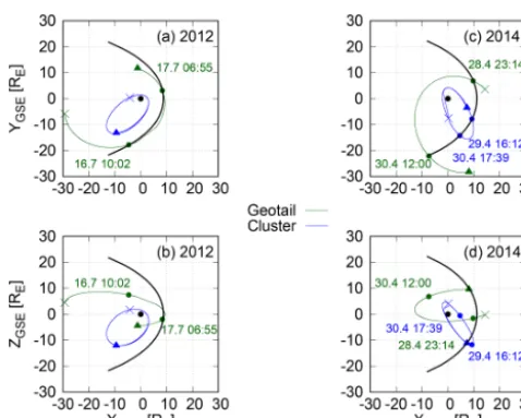
[image:5.612.129.469.403.641.2]Figure 3.Orbits of Cluster 1 (blue) and Geotail (green) satellites during 14 July 09:00 UT–17 July 15:00 UT, 2012(a, b)and during 28 April 19:00 UT–1 May 17:00 UT, 2014(c, d). Orbits are shown on theXYplane in panels(a)and(c)and on theXZplane in pan-els (b) and (d). The coordinate system is GSE. The most earth-ward position of the Shue magnetopause during both time inter-vals is drawn in black. Start and end points of the time interinter-vals are marked with a cross and a triangle, respectively. The points along the satellite orbits between which the spacecraft may encounter magnetopause crossings are marked with dots.
the magnetopause location (black) from the empirical Shue model (Shue et al., 1997) on theXY plane (Fig. 3a and c) and on theXZ plane (Fig. 3b and d) for both events. The netopause position is computed for the most earthward mag-netopause location during the events, while the orbit tracks include intervals of nominal upstream conditions before and after the ICME events. Start and end points of the time in-tervals are marked with a cross and a triangle, respectively. Dots mark the points where satellite orbits intersect (located visually) the innermost position of the magnetopause. The variability of the magnetopause position means that between those orbit tracks the S/C may cross to outside the mag-netosphere. The used coordinate system is GSE. Based on Fig. 3, the Cluster spacecraft orbits inside of the magneto-sphere throughout the 2012 event and for most of the 2014 event. On the other hand, Geotail is outside the magneto-sphere an extended period during 16–17 July 2012 as well as during several periods in April–May 2014.
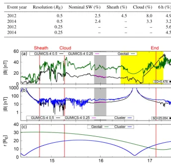
Figures 4 and 5 show time series of the magnetic field magnitude |B| along the Geotail (panel a) and Cluster (panel b) orbits during the 2012 and 2014 events. Green (Geotail) and blue (Cluster) curves show the observations, while the black (magenta) curve shows the magnetic field magnitude along the spacecraft orbits in GUMICS-4 simu-lation using 0.5 (0.25)REmaximum spatial resolution. The yellow-shaded regions in panels (a) and (b) indicate times when the spacecraft may encounter magnetopause
cross-ings. Note that a logarithmic scale is used for the Cluster data. Panel (c) in both figures shows the radial distance of the spacecraft from the center of the Earth. Note that satel-lite measurements have been interpolated over long (several hours) data gaps, most notably on 16 July, 12:15–18:45 UT.
At the start of the 2012 event, Geotail resides in the plasma sheet but quickly moves to the boundary layer (roughly 14 July, 16:00 UT to 15 July, 06:00 UT), after which it en-ters the lobe as the cloud proper hits the magnetosphere. At around the end of the data gap at the end of 16 July, the space-craft moves to the low-latitude boundary layer and the mag-netosheath (identified from plasma data not shown here).
At the start of the 2012 event, Cluster is near perigee, recording field values dominated by the dipole contribution. Cluster exits the ring current region around 16:00 UT on 14 July and enters the plasma sheet. A brief encounter in the lobe is recorded between roughly 18:00 UT 15 July and 06:00 UT 16 July. A second period in the inner magneto-sphere commences around 12:00 UT on 16 July, with exit to the lobe after 00:00 UT 17 July (identified from plasma and energetic particle data not shown here).
4 Analysis
4.1 Global dynamics
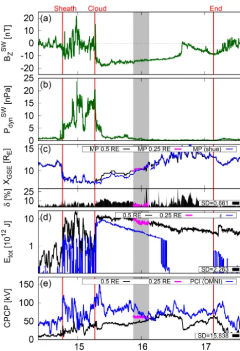
Figures 6 and 7 show the effect of upstream IMFBZ(panel a) and solar wind dynamic pressure (panel b) on the magne-topause nose (panel c), total energy through the dayside mag-netopause nose position (panel d) and the ionospheric CPCP (panel e) during the simulated intervals shown in Figs. 1 and 2. The 0.5REresolution run results are shown in black, and 0.25REresolution results are shown in magenta. The grey-shaded area highlights the 6 h interval simulated using both resolutions. Blue and green curves indicate reference values (see below) and solar wind upstream conditions, respectively. As a metric for validating the simulation results, we use the magnitude of the relative difference (given asδin panel c of Figs. 6 and 7)
δ=
xref−xGUMICS-4 xref
, (2)
in whichx is the GUMICS-4 variable andxrefrefers to the reference parameter value of the variable. An averageδvalue is computed for each ICME simulation phase (nominal solar wind, sheath, cloud) for both 0.5REand 0.25REresolution runs. These percentage values can be found in Table 2. We also compute the standard deviation (SD) for the reference vs. GUMICS-4 results. A single SD value (given in panels c, d and e) is computed for the 0.5REresolution runs to illus-trate how similar the temporal evolution is over timescales of days for GUMICS-4 and the reference parameter.
con-Table 2.Average relative difference magnitudes in the magnetopause nose position for a given simulation phase.
Event year Resolution (RE) Nominal SW (%) Sheath (%) Cloud (%) 6 h (%)
2012 0.5 2.5 4.5 8.0 4.9
2014 0.5 2.4 – 3.3 3.2
2012 0.25 – – – 5.6
2014 0.25 – – – 4.5
Figure 4.The time series of the magnetic field magnitude|B|along the orbits of Geotail(a)and Cluster 1(b)during 14 July 09:00 UT– 17 July 15:00 UT, 2012 as measured by Geotail (green) and Cluster 1 (blue) and predicted by GUMICS-4 (black and magenta). Black and magenta curves in panels(a)–(b)show GUMICS-4 results with maximum spatial resolutions of 0.5 (black) and 0.25 (magenta)RE.(c)Radial distance of both spacecraft from the center of the Earth. Yellow-shaded regions indicate approximate time intervals when a satellite may exit the magnetosphere. Grey-shaded regions show the part of the ICME event simulated also using 0.25REmaximum spatial resolution. Standard deviations (SDs) for observation vs. GUMICS-4 (0.5REresolution) datasets are given in panels(a)and(b).
ditions, while the solar wind dynamic pressure is steady and low. At the onset of ICME sheath, both BZ and dynamic pressure start fluctuating with increased amplitude. More-over, after the onset of ICME cloud, the orientation of the IMF slowly rotates from southward to northward, with the solar wind dynamic pressure decreasing rapidly and remain-ing low until the end of the simulated interval. This behavior is somewhat similar during the 2014 event (Fig. 7a–b), with the exception of missing high-amplitude fluctuations due to the absence of a distinct ICME sheath.
In GUMICS-4, we identify the magnetopause nose posi-tion as a single grid point with the maximum value of JY along the Sun–Earth line, using 1 min temporal resolution, smoothed using 10 min sliding averages. This value is com-pared with the Shue et al. (1997) empirical magnetopause model. For simplicity, the nose of the magnetopause is re-ferred to as a magnetopause. Figure 6c shows that at the
onset of ICME sheath, the magnetopause moves earthward as a consequence of changing upstream conditions, which is followed by sunward return motion lasting until the end of the ICME event. The averageδ is highest during the cloud (8 %) and lowest (2.5 %) during nominal solar wind condi-tions. During ICME sheath, averageδ is 4.5 %. During the 2014 event, the magnetopause starts moving earthward at least 10 h before the onset of ICME cloud (Fig. 7c), as the dynamic pressure increases, with IMFBZ staying positive. After the onset however the magnetopause moves sunward for a few hours until slowly moving earthward again. The dif-ference in averageδbetween cloud and nominal solar wind conditions is lower than for the 2012 event, as the respective values are 3.3 % and 2.4 %.
[image:7.612.125.471.82.414.2]Figure 5.The time series of the magnetic field magnitude|B|along the orbits of Geotail(a)and Cluster 1(b)during 28 April 19:00 UT– 1 May 17:00 UT, 2014 as measured by Geotail (green) and Cluster 1 (blue) and predicted by GUMICS-4 (black and magenta). Black and magenta curves in panels(a)–(b)show GUMICS-4 results with maximum spatial resolutions of 0.5 (black) and 0.25 (magenta)RE.(c)Radial distance of both spacecraft from the center of the Earth. Yellow-shaded regions indicate approximate time intervals when a satellite may exit the magnetosphere. Grey-shaded regions show the part of the ICME event simulated also using 0.25REmaximum spatial resolution. SDs for observation vs. GUMICS-4 (0.5REresolution) datasets are given in panels(a)and(b).
of the Shue et al. (1997) model (blue curve). During the last 2 h, however, there are more fluctuations in the GUMICS-4 magnetopause position, especially in the 0.5REresolution run. From 15 July, 21:00 UT to 16 July, 01:00 UT the simu-lation runs agree on the magnetopause location and also with the Shue model, with differences within 10 % all the time of the first 4 h. However, the last 2 h show more variations between the three curves: the finest resolution shows slight outward motion of the magnetopause, which toward the end of the period is less than that predicted by the Shue model. On the other hand, the 0.5RE resolution run shows inward indentations followed by outward motion consistent with the Shue model. Overall, the 0.5REresolution run is 58 % of the time within 10 % of the Shue model, and the 0.25RE reso-lution run agrees 67 % of the time within 10 % of the Shue model. Despite the fact that the average relative difference is slightly lower for the 0.5REresolution run (4.9 %) than for the 0.25RE resolution run (5.6 %), over the entire 6 h peri-ods, the 0.25RErun is within 10 % of the Shue model 92 % of the time, while the 0.5RErun reaches within 10 % of the Shue model 89 % of the time due to the 0.5RE run being more inclined toward moving more earthward during the last 2 h of the 6 h period.
The time evolution of the magnetopause position during the 6 h period in Fig. 7 is similar for both spatial reso-lutions, with both simulation runs responding similarly to
small upstream fluctuations. Both simulation runs stay within 10 % of the Shue model prediction for the entire 6 h period. The average relative difference is only slightly lower for the higher-resolution run (3.2 %) than for the lower-resolution run (4.5 %).
Overall, the higher-resolution run yielded better agree-ment with the magnetopause location, especially for a mov-ing magnetopause nose (2012 event), because increasmov-ing the spatial resolution sharpens the gradients and allows bet-ter identification of the locations of the maxima (Janhunen et al., 2012). Comparison of the runs shows, however, that the results are consistent with each other, indicating that the lower-resolution run provides similar large-scale dynamics to the finer-resolution run. Furthermore, increasedδduring the 2012 ICME cloud and overall higherδduring the 2012 event indicate that GUMICS-4 accuracy in the magnetopause nose position prediction is better during weaker solar wind driv-ing. This is further demonstrated by the standard deviation values, which are 0.661 for the 2012 event and 0.321 for the 2014 event (see Figs. 6c and 7c).
Total energy through the dayside magnetopause is com-puted by evaluating the energy flux incident at the (Shue) magnetopause, and it is evaluated from
K=
u+p− B 2
2µ0
V+ 1
µ0
Figure 6. (a) Interplanetary magnetic fieldZcomponent,(b) so-lar wind dynamic pressure,(c)distance to the nose of the magne-topause,(d)energy transferred from the solar wind into the magne-tosphere through the dayside magnetopause, and(e)the cross-polar cap potential during 15 July 21:00 UT–16 July 03:00 UT, 2012. Ma-genta plots in panels(c)–(d)show results with a maximum spatial resolution of 0.25RE. Blue curves in panels(c),(d), and(e)show the reference values (the Shue model, theparameter, the PCI). The relative difference magnitudeδbetween GUMICS-4 and the refer-ence value is shown in panel(c). SDs for reference vs. GUMICS-4 (0.5REresolution) datasets are given in panels(c)–(e).
whereuis the total energy density,ppressure,B magnetic field, V flow velocity andE×B the Poynting flux and its component perpendicular to the magnetopause surface. As is shown in Fig. 6c, the relative difference magnitude δ in the magnetopause nose location can reach up to 30 % val-ues. To avoid underestimating the size of the magnetosphere, we evaluate the magnetopause surface by moving the radial distance of each Shue magnetopause surface value 30 % fur-ther away from the Earth. This surface is then used in in-tegrating the energy flux values entering the magnetosphere sunward of the terminator (X >0RE). The results are shown for the 2012 event in Fig. 6d for both 0.5 and 0.25RE reso-lution runs along with the computed parameter (Perreault
Figure 7. (a)Interplanetary magnetic fieldZcomponent,(b) so-lar wind dynamic pressure,(c)distance to the nose of the magne-topause,(d)energy transferred from the solar wind into the magne-tosphere through the dayside magnetopause, and(e)the cross-polar cap potential during 30 April 00:00–06:00 UT, 2014. Magenta plots in panels(c)–(d)show results with a maximum spatial resolution of 0.25RE. Blue curves in panels(c),(d), and(e)show the reference values (the Shue model, theparameter, the PCI). The relative dif-ference magnitudeδbetween GUMICS-4 and the reference value is shown in panel(c). SDs for reference vs. GUMICS-4 (0.5RE reso-lution) datasets are given in panels(c)–(e).
and Akasofu, 1978):
=4π
µ0
V B2sin4
θ
2
l02, (4)
whereµ0 is vacuum permeability,B andV are the magni-tudes of the IMF and solar wind plasma flow velocity,θis the IMF clock angle, andl0 is an empirically determined scale length.
[image:9.612.50.288.63.411.2] [image:9.612.313.548.63.411.2]Thus the relative difference is not a good metric to describe the difference between GUMICS-4 and theparameter, and thus we are not using it in this paper. However, general tem-poral evolution is similar for most parts of ICME cloud, with both GUMICS-4 and theparameter reproducing steep in-crease at the onset of cloud as well as subsequent slow de-crease, as is shown by the computed SD value in Fig. 6d (2.263). As in the case of the 2012 event, the two simulation runs using different spatial resolutions are almost inseparable in terms of the incoming solar wind energy during the 2014 event (Fig. 7d). During moderate solar wind driving in 2014, GUMICS-4 is closer to theparameter, with a considerably lower SD value (0.725) compared with the 2012 event. This is an interesting characteristic of theparameter warranting further study.
Differences between the simulations executed using differ-ent spatial resolutions in local measures, such as the magne-topause nose position, do not show in global variables, such as the total energy through the dayside magnetopause sur-face. As can be seen in Fig. 6d, the curves of the two differ-ent spatial-resolution runs are almost iddiffer-entical. This empha-sizes that integrated quantities, such as energy, give a better representation of the true physical properties of the magneto-sphere in the GUMICS-4 solution and are not dependent on grid resolution (Janhunen et al., 2012). We acknowledge that using more sophisticated methods for identifying the magne-topause surface from the simulation could potentially lead to some changes in the results. The Shue model was used for its simplicity and computational ease. Our results agree in gen-eral with Palmroth et al. (2003), who identified the magne-topause by using plasma flow streamlines from GUMICS-4, indicating that the use of the Shue model does not introduce large errors into the energy estimates.
The magnetosphere–ionosphere coupling, here illustrated by the CPCP time evolution in Fig. 6e, is compared with the polar cap index (Ridley and Kihn, 2004) computed as PCI=29.28−3.31 sin(T+1.49)+17.81PCN, (5) where T is month of the year normalized to 2π and PCN is the northern polar cap index retrieved from OMNIWeb. The PCI is a very indirect proxy (based on a single-point measurement only) for the CPCP, and thus the comparisons must be interpreted with great care. Also, taking into account that one of the well-known features of GUMICS-4 is lower predicted CPCP values compared with its contemporaries (Gordeev et al., 2015), it is of little importance to report the relative differences in CPCP values with the PCI as a refer-ence. However, in terms of the SD values, GUMICS-4 and the PCI show better agreement in the temporal evolution of CPCP during the 2014 event (SD=15.838) than during the 2014 event (SD=5.107). It is apparent that these SD values are clearly the highest of all three (magnetopause nose, en-ergy, CPCP) for both events. This is in part due to the iono-spheric (local) processes contributing to the PCI, but is not related to the large-scale potential evolution.
4.2 Saturation of the cross-polar cap potential
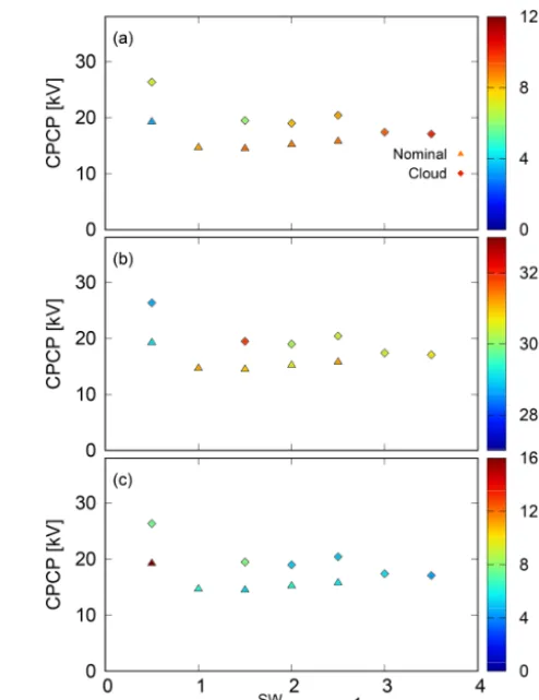
Figures 8 and 9 show the CPCP (both the Northern Hemi-sphere and the Southern HemiHemi-sphere) as a function of the so-lar wind electric fieldEY component for both ICME events. Color-coding marks the IMF magnitude in Figs. 8a and 9a, solar wind speed in Figs. 8b and 9b, and the upstream Alfvén–Mach number in Figs. 8c and 9c. Every data point in Fig. 8 (Fig. 9) is computed from 10 min averages, binned byEY with 1.0 (0.5) mV m−1 intervals. The ICME sheath (solid circles) and cloud (solid squares) periods as well as the nominal solar wind conditions (solid triangles) prior to and following the events are analyzed separately. Note that here only the coarse grid (0.5RE) simulation results are used, as we analyze the effects during the entire magnetic cloud and sheath periods, including times before and after the event not covered by the high-resolution run.
Figure 8 shows that the response of the CPCP to the up-streamEY is quite linear during the magnetic cloud (squares) when solar wind driving electric fieldEYis below 5 mV m−1, during nominal solar wind conditions (triangles) and ICME sheath (diamonds). However, the polar cap potential first de-creases and subsequently saturates during the cloud when the solar wind driving is stronger (EY >5 mV m−1). For the 2012 event, we refer to theEY range from 0 to 5 mV m−1as the linear regime, and from 5 mV m−1upward as the nonlin-ear regime.
Figure 8a shows the obvious result that the highestEY val-ues are associated with the highest IMF magnitudes. How-ever, it also shows that the largest IMF magnitudes are asso-ciated with the nonlinear regime, indicating that strong up-stream driving leads to CPCP saturation. In addition, Fig. 8b suggests that the increase in the CPCP in the linear regime is clearly higher for lower velocity values (cloud structure) than for higher velocity values (sheath and nominal conditions). Generally, this agrees with the previous studies utilizing sta-tistical (Newell et al., 2008) and numerical (Lopez et al., 2010) tools. The latter authors suggest that this is caused by the solar wind flow diversion in the pressure-gradient-dominated magnetosheath; faster solar wind will produce more rapid diversion of the flow around the magnetosphere, and thus a smaller amount of plasma will reach the magnetic reconnection site.
Figure 8.The cross-polar cap potential (CPCP) as a function of the IMFEY for the 2012 ICME sheath and cloud periods, with nomi-nal solar wind conditions before and after the ICME event taken into account separately. GUMICS-4 simulation data with 1 min time res-olution have been averaged by 10 min and binned by upstreamEY with 1.0 mV m−1intervals. Panels(a),(b)and(c)show the mag-nitudes of the IMF, the upstream flow speed and the Alfvén–Mach number, respectively.
Figure 9 agrees with the view presented above, as the response of the CPCP to the upstream EY during the 2014 event is quite linear regardless of the IMF magnitude (Fig. 9a), plasma flow speed (Fig. 9b), or large-scale solar wind driving structure (ICME cloud or nominal solar wind). This is apparently because solar wind driving is substantially weaker during the 2014 event than during the 2012 event, with the IMF magnitude reaching barely 10 nT and upstream plasma flow speed varying only on the order of 10 km s−1. As a result, the upstream Alfvén–Mach number is MA>4 throughout the ICME event as well as during the nominal solar wind conditions. The high polar cap potential values for the lowestEY bin are associated with the large density enhancement driving polar cap potential increase before the arrival of the cloud proper.
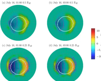
[image:11.612.48.300.65.381.2]Figure 10 shows the region 1 and region 2 field-aligned current (FAC) system coupling the magnetosphere and the ionosphere (e.g., Siscoe et al., 1991). The four panels show
Figure 9.The CPCP as a function of the IMF EY for the 2014 ICME cloud period, with nominal solar wind conditions before and after the ICME event taken into account separately. GUMICS-4 simulation data with 1 min time resolution have been averaged by 10 min and binned by upstreamEYwith 0.5 mV m−1intervals. Pan-els(a),(b)and(c)show the magnitudes of the IMF, the upstream flow speed and the Alfvén–Mach number, respectively.
Figure 10.The Northern Hemisphere field-aligned current pattern in GUMICS-4 simulation at 01:00 UT(a, c)and at 03:00 UT(b, d)on 16 July 2012. Panels(a)and(b)or(c)and(d), respectively, show the results of the simulation run in which 0.5 or 0.25REmaximum spatial resolution was used.
4.3 Local dynamics
Figures 4 and 5 show the time series of the IMF magnitude |B| in the Geotail and Cluster orbits during the 2012 and 2014 events compared with the GUMICS-4 results along the satellite tracks. The standard deviations are computed using the same methods as in Sect. 4.1, and are given in panels (a) and (b). Since the inner boundary of the GUMICS-4 MHD region is at 3.7RE, the times when Cluster is closer than 3.7REto Earth are ignored when computing SD values.
Prior to the arrival of the sheath region in 2012, Geotail enters the plasma sheet boundary layer earlier than predicted by GUMICS-4. During the ICME sheath there are many dips and peaks in both plots, with the difference between measured (both Geotail and Cluster) and predicted values varying, as can be seen from Fig. 4a and b. Also, Fig. 4a shows that starting from 17 July, 06:00 UT, the measured field at Geotail increases as the satellite goes to the magne-tosheath proper, while GUMICS-4 prediction decreases as the orbit track in GUMICS-4 approaches the shock region (see Fig. 3a). The 2014 event shows similar features, espe-cially when Geotail enters and exits the magnetosphere at 23:14 UT, 28 April, and at 12:00 UT, 30 April, respectively, with measured (by Geotail)|B|in the former case fluctuating and rising sharply from 10 to 40 nT, while the GUMICS-4 |B|increases more steadily from a few to 20 nT as the satel-lite enters from the magnetosheath to the magnetosphere. In
the latter case decrease (increase) in measured (simulated) |B|occurs several hours after the spacecraft exits the mag-netosphere (later yellow-shaded region in Fig. 5a) because of the differences in the moment of exit (and exact loca-tion of the magnetopause localoca-tion). Note that while Cluster makes an entry into the magnetosphere at 16:12 UT, 29 April, GUMICS-4 predicts a position within the magnetosheath and an entry into the magnetosphere only following the end of the cloud.
Note that the Cluster perigee (2RE) (Fig. 4c) is below the inner boundary of the GUMICS-4 simulation (3.7RE), which causes the simulation field to record unphysical val-ues around the time of the maxima at 09:00 on 14 July 2012 and 15:00 on 16 July 2012, hence the data gaps in GUMICS-4 data plots.
The effect of the ICME sheath is visible after its arrival in Fig. 4, with both measured and predicted|B|fluctuation. The ICME magnetic cloud proper seems to cause the largest difference in|B|during the 2012 event, when the driving was quite strong.
5 Discussion
In this paper we study (1) how the magnetosphere responds to two ICME events with different characteristics by means of using the GUMICS-4 global MHD simulation and (2) how accurately GUMICS-4 reproduces the effects of the two events. The 2012 event was stronger in terms of solar wind driver, the 2014 event being significantly weaker in terms of both solar wind speed and IMF magnitude. We considered both global and local parameters, including magnetopause nose position along the Sun–Earth line, total energy trans-ferred from the solar wind into the magnetosphere, and the ionospheric cross-polar cap potential (CPCP). Local mea-sures include response of the magnetic field magnitude along the orbits of Cluster and Geotail spacecraft. The two ICME events were simulated using 0.5RE maximum spatial res-olution. To test the effect of grid-resolution enhancement on global dynamics, we simulated 6 h subsets of both CME cloud periods with 0.25REmaximum spatial resolution. As uncertainty metrics we use both relative difference magni-tudeδand SD.
Due to stronger solar wind driving, the 2012 event causes the magnetosphere to compress more than during the 2014 event, with the magnetopause moving earthward at the onset of the 2012 ICME sheath and reaching 7RE distance from Earth, until moving sunward at the onset of ICME magnetic cloud (see Fig. 6c). Both ICMEs are preceded by low IMF
BZ and solar wind dynamic pressure, with 2014 missing high-amplitude fluctuations before ICME cloud due to the absence of a separate ICME sheath. Despite this, the move-ment of the magnetopause is similarly earthward prior to the cloud, reaching 9.5REjust before the onset of the cloud (see Fig. 7c). During the cloud, however, the orientation of the IMF slowly rotates from southward to northward and the magnetopause is in constant sunward (earthward) motion in 2012 (2014). While the polarity of the IMF changes before the end of the ICME in 2012, it changes from southward to northward only after the end of the ICME in 2014.
The magnetopause nose location in GUMICS-4 is identi-fied as a single grid point from the maximum value of JY along the Sun–Earth line. Location deviations in response to solar wind driving in the GUMICS-4 results are depen-dent on the driver intensity: stronger driving during the 2012 CME magnetic cloud leads to a larger relative difference magnitudeδ (2012: 8.0 %δ on average) as compared to the Shue et al. (1997) model, whereas the agreement between the simulation and the empirical model is quite good (3.3 %
δ on average) during weaker driving during the 2014 event (Figs. 6 and 7). This view is further supported by SDs: for the full simulation time range, the SD is 0.661 (0.321) in 2012 (2014). Averageδduring nominal solar wind conditions is al-most identical for both events: 2.5 % for the 2012 event and 2.4 % for the 2014 event.
Comparison of the magnetopause location between the 0.25RE(0.5RE) resolution run and the Shue model shows
that the relative difference between the two is below 10 % for 92 % (89 %) of the 6 h subset in 2012 (Fig. 6c), while corresponding analysis of the 6 h subset in 2014 (Fig. 7c) yielded differences below 10 % for 100 % of the time re-gardless of the resolution. It should be noted that, despite the relative difference in magnitude being slightly lower for the 0.5REresolution run than for the 0.25REresolution run for both the 2012 (4.9 % and 5.6 %) and 2014 (3.2 % and 4.5 %) events, the 0.25RE run reaches better agreement with the Shue model, especially when the magnetopause is moving during high solar wind driving in 16 July, 01:00 UT (Fig. 6c). When spatial resolution is increased, gradient quantities such as JY have sharper profiles and therefore larger val-ues (Janhunen et al., 2012). As it is the maximum value of
JY that we use to locate the magnetopause nose, the nose position evaluation in the lower-resolution runs is more am-biguous due to the larger spread of the current and due to the larger grid cell size. This may lead to changes in the maximum value of up to severalREover short time periods in response to upstream fluctuations. In the finer-resolution runs, JY distribution is sharper, which leads to lesser fluc-tuations in the maximum value determination. However, the differences between the two grid resolutions occur only un-der rapidly varying solar wind or very low solar wind density conditions.
The empirical models developed by Shue et al. (1997, 1998) are based on statistical analysis of a large number of spacecraft measurements of plasma and magnetic field dur-ing magnetopause crossdur-ings. While the Shue et al. (1997) model is optimized for moderate upstream conditions, the Shue et al. (1998) model targets especially stronger driving periods. However, we computed the difference in the mag-netopause position between the two models and found that it is mostly less than 0.1REwith a maximum difference of 0.4RE, with the Shue et al. (1997) model predicting more sunward magnetopause nose. Because of the small differ-ence at the magnetopause nose, we have only used the Shue et al. (1997) model in our study. Our results agree with pre-vious papers (Palmroth et al., 2003; Lakka et al., 2017), with the latter reporting a 3.4 % average relative difference be-tween the Shue model and GUMICS-4. Moreover, according to Gordeev et al. (2015), global MHD models are very close to each other in terms of predicting magnetopause standoff distance.
bet-ter to consider such global integrated quantities, even if they have no direct observational counterparts. This can be seen in Figs. 6d and 7d, with large differences between GUMICS-4 and theparameter (Perreault and Akasofu, 1978) in en-ergy transferred from the solar wind into the magnetosphere in both 2012 and 2014. However, standard deviations show that GUMICS-4 reproduces the temporal evolution of the
parameter better during low solar wind driving (2014) than during high driving (2012), as the respective SD values are 0.725 and 2.263. Moreover, our results are mostly on the same order of magnitude compared to what was obtained by Palmroth et al. (2003) by using plasma flow streamlines for computing the magnetopause surface from GUMICS-4 re-sults.
In the ionosphere, the cross-polar cap potential value is de-pendent on the grid resolution, with higher resolution yield-ing higher polar cap potential values (see Figs. 6e and 7e). In comparison with the PCI (Ridley and Kihn, 2004), standard deviation is considerably lower for the 2014 event (5.107) than for the 2012 event (15.838). Thus, at least two factors contribute to the ionospheric coupling: grid resolution and intensity of solar wind driving. Considering that the SD val-ues are clearly higher than, e.g., the corresponding energy transfer values and that the PCI considers only the Northern Hemisphere, the PCI may not provide the most accurate ref-erence for GUMICS-4. However, both considerable differ-ence between GUMICS-4 and the PCI and the dependdiffer-ence on grid resolution agree with previous studies (e.g., Lakka et al., 2018). Generally, global MHD codes differ from each other in terms of the CPCP values (Gordeev et al., 2015). It is not easy to reproduce realistic CPCP values in a global MHD code, since they are generally prone to close excessive amounts of electric current through the polar cap and thus the CPCP values are either unrealistically large (e.g., LFM model, Lyon et al., 2004), with reasonable auroral electrojet currents, or reasonable accompanied by low auroral electro-jet currents (De Zeeuw et al., 2004) (e.g., GUMICS-4 and BATS-R-US model; Powell et al., 1999).
The polar cap structure and the distribution of the FAC do not change much in either of the simulations, thus suggesting that the coupling of the magnetosphere and the ionosphere remains relatively constant. As is shown in Fig. 10a–b, the region 1 currents are clearly visible, while the region 2 cur-rents get stronger only by enhancing the grid resolution in the MHD region (Janhunen et al., 2012). However, the up-stream conditions change considerably from 01:00 to 03:00, with the upstream Alfvén–Mach number decreasing from 1.9 to 0.6, suggesting that polar cap potential saturation mecha-nisms are likely to take place (Ridley, 2007; Wilder et al., 2015; Lakka et al., 2018). Considering that GUMICS-4 re-produces saturation with both 0.5RE(this paper) and 0.25RE resolutions (Lakka et al., 2018), it is apparent that the FAC influence on the dayside magnetospheric magnetic field does not contribute to the saturation effect. However, to actually prove it is beyond the scope of the current paper. We
there-fore conclude that the increase in the CPCP during the 0.5RE simulation run is caused by processes outside of the magne-tosphere, likely in the magnetosheath, and that GUMICS-4 responds differently to low Alfvén–Mach number solar wind depending on grid resolution.
Figures 8 and 9 illustrate the CPCP as a function of the solar windEY component. Color-coded are the IMF mag-nitude in Figs. 8a and 9a, the solar wind speed in Figs. 8b and 9b, and the upstream Alfvén–Mach number in Figs. 8c and 9c. Nominal solar wind conditions before and after the actual ICME events as well as the ICME sheath and cloud periods are considered separately. We note that only results from the lower spatial resolution (0.5RE) runs are included in the figures. Consistent with earlier studies, Fig. 8 shows saturation of the CPCP during high solar wind driving (see, e.g., Shepherd, 2007; Russell et al., 2001): with nominal so-lar wind conditions or during the ICME sheath period the response of the CPCP to the upstreamEY is rather linear, while for the ICME cloud period the CPCP saturates when
EY >5 mV m−1. From Fig. 8a it can be seen that the sat-uration occurs whenB >12 nT and Fig. 8b shows that the increase in the CPCP in the linear regime depends on the upstream velocity in such a way that the increase is clearly higher for lower velocity values (cloud event) than for higher velocity values (sheath event and nominal conditions), as suggested by previous statistical (Newell et al., 2008) and numerical (Lopez et al., 2010) studies. The latter study pro-poses that this is because of the more rapid diversion of the solar wind flow in the pressure-gradient-dominated mag-netosheath under faster solar wind, which leaves a smaller amount of plasma at the magnetic reconnection site.
The saturation of the CPCP is absent in Fig. 9 due to the significantly weaker solar wind driving during the 2014 event (the upstream EY is below 4 mV m−1). This in turn leads to the upstream Alfvén–Mach number being on average 5.8 during the ICME cloud event. Lavraud and Borovsky (2008) suggest that when the Alfvén–Mach number decreases below 4 and the overall magnetosheath plasma beta (p/pB, wherep is the plasma pressure andpBthe magnetic pressure) below 1, the magnetosheath force balance changes such that plasma flow streamlines are diverted away from the magnetic recon-nection merging region in the dayside magnetopause (Lopez et al., 2010), which causes the CPCP saturation. However, the CPCP saturation limit ofMA=4 is not necessarily the only governing parameter, as there is both observational evi-dence with largeMAvalues (up to 7.3) (Myllys et al., 2016) and simulation results indicating saturation at low but above
MA=1 values (this study). Nonetheless, our results suggest that the saturation of the CPCP is dependent on the upstream
MAin such a way thatMAneeds to be below 4 for the satu-ration to occur.
This is actually apparent in Fig. 1h as well: the absolute values of both BZ andVX reach their maximum values a few hours after the onset of the magnetic cloud, which is at 06:54 UT, 15 July. However, the CPCP is at that time quite moderate, about 40 kV, and does not reach its maximum until 16 July, when bothBZandVXhave already reduced signifi-cantly. Thus the CPCP overshoots in Fig. 8, a feature that was not observed in a GUMICS-4 study by Lakka et al. (2018) using artificial solar wind input consisting of relatively high-density and constant driving parameters.
The performance of GUMICS-4 was put to the test by means of comparing the magnetic field magnitude |B| to in situ data of the Cluster and Geotail satellites. GUMICS-4 values are mostly lower than those measured by either of the two spacecraft, with GUMICS-4 predictions being closer to Cluster than Geotail. Computed standard deviations re-veal that, over the entire simulation periods, the temporal evolution of GUMICS-4 magnetic field magnitude predic-tions is closer to Geotail measurements (2012: SD=5.476, 2014: SD=6.564, equatorial orbit) than Cluster measure-ments (2012: SD=25.054, 2014: SD=24.795, polar orbit) for both events. It should be noted that the times when Clus-ter is closer than 3.7REto Earth are ignored when computing SD values due to the inner boundary of the GUMICS-4 MHD region, which is located at 3.7RE.
During both events, |B| is increased during ICMEs, es-pecially their magnetic cloud counterparts. During the 2012 ICME sheath both Cluster and Geotail record fluctuating|B| until the onset of the cloud. While missing a sheath in 2014, magnetic field magnitude measured by Cluster fluctuates as well prior to the cloud. At the same time (29 April, 15:00 UT) |B| measured by Geotail decreases sharply. The difference between Cluster/Geotail and GUMICS-4 is mostly on the or-der of 10 % but can reach above 50 % values, especially dur-ing the 2012 magnetic cloud event in both Cluster and Geo-tail orbit. Such a difference seems relatively large, especially since it was shown by Ridley et al. (2016) that all the global MHD models available at the Community Coordinated Mod-eling Center (CCMC) are close to each other when compar-ing the ability to reproduce magnetic field components to in situ measurements. While the study used 662 simulation runs, it should be noted that GUMICS-4 was used in only 12 of them. However, GUMICS-4 should predict|B|closer to in situ measurements at least during moderate solar wind driv-ing, as was shown by Facskó et al. (2016). In his work the difference in |B| was 10 % or lower on 20 February 2002, when no ICME events were recorded.
With such discrepancy between our results and previ-ous results, we checked some of the simulation runs at CCMC, in which BATS-R-US (Powell et al., 1999) code was used, and searched for runs of either of the two ICME events discussed in this paper, with magnetic field mea-surements along Geotail and/or Cluster orbit also available. BATS-R-US was chosen since it shares several features with GUMICS-4. We found one simulation run (CCMC run
name Tom_Bridgeman_022415_1) in which the 2012 event was simulated, with results along Geotail orbit available. In addition, we simulated the 2014 event (CCMC run name Antti_Lakka_070918_2) to check the results along Cluster path. Consequently, we are able to compare GUMICS-4 and BATS-R-US in both 2012 (Geotail) and 2014 (Cluster), and the results are shown in Fig. 11. Panel (a) shows compar-ison between the two models during the 2012 event and panel (b) during the 2014 event. In situ measurements by Geotail and Cluster are shown in panels (a) and (b), respec-tively. Note that the 2012 BATS-R-US run was completed at around 17 July 00:00 UT. By looking at the figure it is appar-ent that the predictions of both GUMICS-4 and BATS-R-US are quite similar, especially during the magnetic cloud events at both Cluster and Geotail orbits. Actually, GUMICS-4 is mostly closer to Cluster measurements than BATS-R-US in 2014, when Cluster exits the magnetosphere and|B| mea-sured by Cluster fluctuates between 10 and 40 nT, as was discussed in Sect. 4.3. In 2012 a large difference in|B|(up to 100 %) during ICME cloud applies to both models. During ICME sheath and nominal solar wind conditions|B| fluctu-ates more and the prediction accuracy of the models depends on the time interval under inspection. It is evident that both models are quite equal considering the ability to reproduce |B|during both 2012 and 2014 ICME events.
The discrepancy between in situ measurements and the two models may not concern only GMHD models, since we computed the magnetic field during the 2012 event at Cluster orbit using the empirical Tsyganenko magnetic field model T89 (e.g., Tsyganenko and Sitnov, 2005). For most parts GUMICS-4 is actually closer to Cluster observations, with the gap between the two models gradually decreasing as Cluster approaches the perigeum on 16 July (not shown). Therefore it is reasonable to assume that something in the ICME event, possibly unusually strong compression, leads to a larger field than predicted by the GMHD models or the Tsyganenko model, and that, e.g., increasing the spatial res-olution of the GMHD models would not make a significant difference for the two reasonably similar codes (Janhunen et al., 2012). The negligible effect of enhanced spatial reso-lution is actually shown in Figs. 4 and 5 for GUMICS-4.
Figure 11.The time series of the magnetic field magnitude|B|along the orbits of Geotail during 14 July 09:00 UT–17 July 15:00 UT 2012(a) and Cluster 1 during 28 April 19:00 UT–1 May 17:00 UT 2014(b)as measured by Geotail (green) and Cluster 1 (blue) and predicted by GUMICS-4 (black) and BATS-R-US (magenta).
however beyond the scope of the current paper and is left for future studies.
We conclude that for both events, |B| predicted by GUMICS-4 is closer to Cluster observations, which fea-ture high magnetic field magnitude outside the plasma sheet. While the differences between GUMICS-4 and in situ mea-surements can be quite large, it was shown that the|B| pre-dicted by GUMICS-4 agrees well with BATS-R-US predic-tions, and thus the large differences are not model-related but rather related to the upstream conditions during the ICME events. Thus the relative difference in|B|may not be a good metric when simulating ICME events and evaluating the per-formance of a global MHD model.
While the agreement between predicted and measured|B| may depend on the upstream conditions, the overall time evo-lutions seem to have a better match, and the SD values sug-gest that GUMICS-4 reproduces temporal evolution of |B| better at Geotail orbit, which is much further away from the Earth than Cluster and resides mostly in the lobe and on the boundary layer. We computed standard deviations for Clus-ter orbit when the S/C is both further and closer than 5RE away from the center of the Earth. SD for further than 5RE is 22.984 (19.666) for the 2012 (2014) event, while for closer than 5RE the SD is 106.337 (104.605) for the 2012 (2014) event. If these calculations are repeated for 6RE distance, the SD values are 14.390 (15.282) when the S/C is further in 2012 (2014) and 104.618 (88.423) when the S/C is closer in 2012 (2014). Thus, the temporal evolutions agree better when Cluster is further away from the Earth.
The differences are most likely not caused by grid cell size variations due to the adaptive grid of GUMICS-4, because the simulation runs over simulated 6 h stages produce quite
similar results for both resolutions. Also, the two runs de-viate most from each other during the first hours of the 6 h stage, during which the 0.25RErun may not have fully elim-inated the effects of simulation initialization, which can pre-vail for hours (Lakka et al., 2017). Moreover, the adaptive grid of GUMICS-4 is enhanced the most near the dayside magnetopause. Both events show signs of increased devia-tion from the measurements near the dayside magnetopause (edges of yellow-shaded regions in Figs. 4 and 5), further manifesting inaccuracies in determining the magnetopause in GUMICS-4.
6 Conclusions
The results of this paper can be summarized as follows. 1. Enhancing spatial resolution of the magnetosphere in
GUMICS-4 affects the accuracy of the determination of the magnetopause subsolar point. Global measures, such as energy transferred from the solar wind into the magnetosphere, are not affected. The cross-polar cap potential can be affected significantly, with up to over a factor of 2 difference between simulations using dif-ferent spatial resolutions for the magnetosphere. 2. Our results show signs of cross-polar cap potential
3. Comparison metric choice should be done cautiously. For instance, relative difference in |B| may not be a good metric when studying ICME events. Due to inac-curacies in the magnetopause subsolar point determina-tion, comparison between GUMICS-4 and in situ data should be done cautiously when the spacecraft is near the magnetopause.
Data availability. Solar wind data are freely available from the NASA/GSFC Omniweb server (https://omniweb.gsfc.nasa.gov/, last access: 30 January 2018). Solar energetic particle data are freely available from the NOAA NCEI Space Weather data ac-cess (https://www.ngdc.noaa.gov/stp/satellite/goes/index.html, last access: 22 March 2018).
Supplement. The supplement related to this article is available online at: https://doi.org/10.5194/angeo-37-561-2019-supplement.
Author contributions. AL performed all the GUMICS-4 simula-tions and prepared manuscript draft versions. TIP contribution was crucial for planning the structure of the paper and enhancing the draft versions. EK assisted with everything related to ICMEs. OR provided solar energetic particle data and helped with the T89 model. IH helped with analyzing GUMICS-4 results. APD, MAL and MP all gave valuable feedback.
Competing interests. The authors declare that they have no conflict of interest.
Acknowledgements. The calculations presented above were per-formed using computer resources within the Aalto University School of Science “Science-IT” project. We acknowledge use of NASA/GSFC’s Space Physics Data Facility’s OMNIWeb service and OMNI data. Solar energetic particle data supplied courtesy of https://ngdc.noaa.gov (last access: 22 March 2018).
Financial support. This research has been supported by the Academy of Finland (Luonnontieteiden ja Tekniikan Tutkimuksen Toimikunta (grant nos. 1267087, 288472 and 310444)).
Review statement. This paper was edited by Elias Roussos and re-viewed by two anonymous referees.
References
Akasofu, S. I.: Energy coupling between the solar wind and the magnetosphere, Space Sci. Rev., 28, 121–190, https://doi.org/10.1007/BF00218810, 1981.
Axford, W. I. and Hines, C. O.: A unifying theory of high-latitude geophysical phenomena and geomagnetic storms, Can. J. Phys., 39, 1433–1464, https://doi.org/10.1139/p61-172, 1961. Birn, J., Drake, J. F., Shay, M. A., Rogers, B. N., Denton, R. E.,
Hesse, M., Kuznetsova, M., Ma, Z. W., Bhattacharjee, A., Otto, A., and Pritchett, P. L.: Geospace Environmental Modeling (GEM) Magnetic Reconnection Challenge, J. Geophys. Res.-Space, 106, 3715–3719, https://doi.org/10.1029/1999JA900449, 2001.
Burlaga, L., Sittler, E., Mariani, F., and Schwenn, R.: Mag-netic loop behind an interplanetary shock: Voyager, Helios, and IMP 8 observations, J. Geophys. Res.-Space, 86, 6673–6684, https://doi.org/10.1029/JA086iA08p06673, 1981.
De Zeeuw, D. L., Sazykin, S., Wolf, R. A., Gombosi, T. I., Ridley, A. J., and Tóth, G.: Coupling of a global MHD code and an inner magnetospheric model: Initial results, J. Geophys. Res.-Space, 109, a12219, https://doi.org/10.1029/2003JA010366, 2004. Dungey, J. W.: Interplanetary Magnetic Field and
the Auroral Zones, Phys. Rev. Lett., 6, 47–48, https://doi.org/10.1103/PhysRevLett.6.47, 1961.
Facskó, G., Honkonen, I., Živkovi´c, T., Palin, L., Kallio, E., Ågren, K., Opgenoorth, H., Tanskanen, E. I., and Milan, S.: One year in the Earth’s magnetosphere: A global MHD simula-tion and spacecraft measurements, Space Weather, 14, 351–367, https://doi.org/10.1002/2015SW001355, 2016.
Goldstein, R., Neugebauer, M., and Clay, D.: A statistical study of coronal mass ejection plasma flows, J. Geophys. Res.-Space, 103, 4761–4766, https://doi.org/10.1029/97JA03663, 1998. Gordeev, E., Sergeev, V., Honkonen, I., Kuznetsova, M.,
Rastät-ter, L., Palmroth, M., Janhunen, P., Tóth, G., Lyon, J., and Wiltberger, M.: Assessing the performance of community-available global MHD models using key system parame-ters and empirical relationships, Space Weather, 13, 868–884, https://doi.org/10.1002/2015SW001307, 2015.
Gosling, J. T.: Coronal Mass Ejections and Magnetic Flux Ropes in Interplanetary Space, 343–364, American Geophysical Union (AGU), https://doi.org/10.1029/GM058p0343, 1990.
Gosling, J. T., Pizzo, V., and Bam, S. J.: Anomalously low proton temperatures in the solar wind following interplanetary shock waves–evidence for magnetic bottles?, J. Geophys. Res., 78, 2001–2009, https://doi.org/10.1029/JA078i013p02001, 1973. Gosling, J. T., McComas, D. J., Phillips, J. L., and Bame, S. J.:
Geomagnetic activity associated with earth passage of interplan-etary shock disturbances and coronal mass ejections, J. Geophys. Res.-Space, 96, 7831–7839, https://doi.org/10.1029/91JA00316, 1991.
Hirshberg, J. and Colburn, D. S.: Interplanetary field and geo-magnetic variations – a unifield view, Planetary Space Science, 17, 1183–1206, https://doi.org/10.1016/0032-0633(69)90010-5, 1969.
Hirshberg, J., Bame, S. J., and Robbins, D. E.: Solar flares and solar wind helium enrichments: July 1965–July 1967, Solar Phys., 23, 467–486, https://doi.org/10.1007/BF00148109, 1972.
On the performance of global magnetohydrodynamic models in the Earth’s magnetosphere, Space Weather, 11, 313–326, https://doi.org/10.1002/swe.20055, 2013.
Huttunen, K. E. J. and Koskinen, H. E. J.: Importance of post-shock streams and sheath region as drivers of intense magnetospheric storms and high-latitude activity, Ann. Geophys., 22, 1729–1738, https://doi.org/10.5194/angeo-22-1729-2004, 2004.
Huttunen, K. E. J., Koskinen, H. E. J., and Schwenn, R.: Variabil-ity of magnetospheric storms driven by different solar wind per-turbations, J. Geophys. Res.-Space, 107, SMP 20-1–SMP 20-8, 2002.
Janhunen, P.: GUMICS-3 A Global Ionosphere-Magnetosphere Coupling Simulation with High Ionospheric Resolution, in: En-vironment Modeling for Space-Based Applications, edited by: Guyenne, T.-D. and Hilgers, A., Vol. 392 of ESA Special Publi-cation, 233 pp., 1996.
Janhunen, P. and Huuskonen, A.: A numerical ionosphere-magnetosphere coupling model with variable con-ductivities, J. Geophys. Res.-Space, 98, 9519–9530, https://doi.org/10.1029/92JA02973, 1993.
Janhunen, P., Palmroth, M., Laitinen, T., Honkonen, I., Ju-usola, L., Facskó, G., and Pulkkinen, T.: The GUMICS-4 global {MHD} magnetosphere–ionosphere cou-pling simulation, J. Atmos. Sol.-Terr. Phy., 80, 48–59, https://doi.org/10.1016/j.jastp.2012.03.006, 2012.
Jianpeng, G., Xueshang, F., Jie, Z., Pingbing, Z., and Changqing, X.: Statistical properties and geoefficiency of interplanetary coronal mass ejections and their sheaths during intense ge-omagnetic storms, J. Geophys. Res.-Space, 115, A09107, https://doi.org/10.1029/2009JA015140, 2010.
Lions, J. L. and Ciarlet, P. G.: Handbook of Numerical Analysis. Solution of Equations in Rn (Part 3), Techniques of Scientific Computing (Part 3), Vol. 7, North-Holland, 1st Edn., Amsterdam, the Netherlands, 2000.
Johnson, J. R. and Cheng, C. Z.: Kinetic Alfvén waves and plasma transport at the magnetopause, Geophys. Res. Lett., 24, 1423– 1426, https://doi.org/10.1029/97GL01333, 1997.
Juusola, L., Facskó, G., Honkonen, I., Janhunen, P., Vanhamäki, H., Kauristie, K., Laitinen, T. V., Milan, S. E., Palmroth, M., Tanskanen, E. I., and Viljanen, A.: Statistical comparison of seasonal variations in the GUMICS-4 global MHD model ionosphere and measurements, Space Weather, 12, 582–600, https://doi.org/10.1002/2014SW001082, 2014.
Kilpua, E., Isavnin, A., Vourlidas, A., Koskinen, H., and Rodriguez, L.: On the relationship between interplanetary coronal mass ejec-tions and magnetic clouds, Living Rev. Sol. Phys., 31, 1251– 1265, 2013.
Kilpua, E., Koskinen, H. E. J., and Pulkkinen, T. I.: Coronal mass ejections and their sheath regions in interplanetary space, Living Rev. Sol. Phys., 14, 5, https://doi.org/10.1007/s41116-017-0009-6, 2017a.
Kilpua, E. K. J., Balogh, A., von Steiger, R., and Liu, Y. D.: Geoeffective Properties of Solar Transients and Stream Interaction Regions, Space Sci. Rev., 212, 1271–1314, https://doi.org/10.1007/s11214-017-0411-3, 2017b.
Koustov, A. V., Khachikjan, G. Ya., Makarevich, R. A., and Bryant, C.: On the SuperDARN cross polar cap po-tential saturation effect, Ann. Geophys., 27, 3755–3764, https://doi.org/10.5194/angeo-27-3755-2009, 2009.
Kubota, Y., Nagatsuma, T., Den, M., Tanaka, T., and Fujita, S.: Polar cap potential saturation during the Bastille Day storm event us-ing global MHD simulation, J. Geophys. Res.-Space, 122, 4398– 4409, https://doi.org/10.1002/2016JA023851, 2017.
Kubyshkina, M., Sergeev, V. A., Tsyganenko, N. A., and Zheng, Y.: Testing Efficiency of Empirical, Adaptive, and Global MHD Magnetospheric Models to Represent the Geomagnetic Field in a Variety of Conditions, Space Weather, 17, 672–686, https://doi.org/10.1029/2019SW002157, 2019.
Lakka, A., Pulkkinen, T. I., Dimmock, A. P., Osmane, A., Honko-nen, I., Palmroth, M., and JanhuHonko-nen, P.: The impact on global magnetohydrodynamic simulations from varying initialisation methods: results from GUMICS-4, Ann. Geophys., 35, 907–922, https://doi.org/10.5194/angeo-35-907-2017, 2017.
Lakka, A., Pulkkinen, T. I., Dimmock, A. P., Myllys, M., Honko-nen, I., and Palmroth, M.: The Cross-Polar Cap Saturation in GUMICS-4 During High Solar Wind Driving, J. Geophys. Res.-Space, 123, 3320–3332, https://doi.org/10.1002/2017JA025054, 2018.
Lavraud, B. and Borovsky, J. E.: Altered solar wind-magnetosphere interaction at low Mach numbers: Coro-nal mass ejections, J. Geophys. Res.-Space, 113, a00B08, https://doi.org/10.1029/2008JA013192, 2008.
Lopez, R. E., Bruntz, R., Mitchell, E. J., Wiltberger, M., Lyon, J. G., and Merkin, V. G.: Role of magnetosheath force balance in regulating the dayside reconnection potential, J. Geophys. Res.-Space, 115, a12216, https://doi.org/10.1029/2009JA014597, 2010.
Lyon, J. G., Fedder, J. A., and Mobarry, C. M.: The Lyon-Fedder-Mobarry (LFM) global MHD magnetospheric sim-ulation code, J. Atmos. Sol.-Terr. Phy., 66, 1333–1350, https://doi.org/10.1016/j.jastp.2004.03.020, 2004.
Myllys, M., Kilpua, E., Lavraud, B., and Pulkkinen, T. I.: So-lar wind-magnetosphere coupling efficiency during ejecta and sheath-driven geomagnetic storms, J. Geophys. Res.-Space, 121, 4378–4396, https://doi.org/10.1002/2016JA022407, 2016. Myllys, M., Kipua, E. K. J., and Lavraud, B.: Interplay of solar
wind parameters and physical mechanisms producing the satu-ration of the cross polar cap potential, Geophys. Res. Lett., 44, 3019–3027, https://doi.org/10.1002/2017GL072676, 2017. Newell, P. T., Sotirelis, T., Liou, K., and Rich, F. J.: Pairs of solar
wind-magnetosphere coupling functions: Combining a merging term with a viscous term works best, J. Geophys. Res.-Space, 113, a04218, https://doi.org/10.1029/2007JA012825, 2008. Nishida, A.: Coherence of geomagnetic DP 2 fluctuations with
in-terplanetary magnetic variations, J. Geophys. Res., 73, 5549– 5559, https://doi.org/10.1029/JA073i017p05549, 1968. Nykyri, K. and Otto, A.: Plasma transport at the
mag-netospheric boundary due to reconnection in Kelvin-Helmholtz vortices, Geophys. Res. Lett., 28, 3565–3568, https://doi.org/10.1029/2001GL013239, 2001.
Osmane, A., Dimmock, A., Naderpour, R., Pulkkinen, T., and Nykyri, K.: The impact of solar wind ULF B-z fluctuations on ge-omagnetic activity for viscous timescales during strongly north-ward and southnorth-ward IMF, J. Geophys. Res.-Space, 120, 9307– 9322, https://doi.org/10.1002/2015JA021505, 2015.