Using Multiple Segmentations for Image Auto-Annotation
Jiayu Tang
Intelligence, Agents, Multimedia Group School of Electronics and Computer Science
University of Southampton, Southampton SO17 1BJ, United Kingdom
[email protected]
Paul H. Lewis
Intelligence, Agents, Multimedia Group School of Electronics and Computer Science
University of Southampton, Southampton SO17 1BJ, United Kingdom
[email protected]
ABSTRACT
Automatic image annotation techniques that try to identify the objects in images usually need the images to be seg-mented first, especially when specifically annotating image regions. The purpose of segmentation is to separate differ-ent objects in images from each other, so that objects can be processed as integral individuals. Therefore, annotation per-formance is highly influenced by the effectiveness of segmen-tation. Unfortunately, automatic segmentation is a difficult problem, and most of the current segmentation techniques do not guarantee good results. A multiple segmentations al-gorithm is proposed by Russellet al.[12] to discover objects and their extent in images. In this paper, we explore the novel use of multiple segmentations in the context of image auto-annotation. It is incorporated into a region based im-age annotation technique proposed in previous work, namely the training image based feature space approach. Three dif-ferent levels of segmentations were generated for a 5000 im-age collection. Experimental results show that imim-age auto-annotation achieves better performance when using all three segmentation levels together than using any single one on its own.
Categories and Subject Descriptors
I.5 [Pattern Recognition]: Miscellaneous
; H.3.1 [Information Storage and Retrieval]: Content Analysis and Indexing
1.
INTRODUCTION
Image auto-annotation, which automatically labels im-ages with keywords, has been gaining more and more at-tentions in recent years. It turns the traditional way of content based image retrieval (CBIR) using low-level im-age features (colour, shape, texture, etc.) as the query, into an approach that is more favorable to people, namely using descriptive words (semantics). Most of the present auto-annotation models predict captions for the whole images [8,
Permission to make digital or hard copies of all or part of this work for personal or classroom use is granted without fee provided that copies are not made or distributed for profit or commercial advantage and that copies bear this notice and the full citation on the first page. To copy otherwise, to republish, to post on servers or to redistribute to lists, requires prior specific permission and/or a fee.
CIVR’07, July 9–11, 2007, Amsterdam, The Netherlands
Copyright 2007 ACM 978-1-59593-733-9/07/0007 ...$5.00.
6, 15], while a few are able to attach words to specific image regions [5, 17, 14]. Annotating images at the whole image level does not indicate which part of the image gives rise to which word, so it is not explicitly object recognition. From this point of view, the second form which generates regional captions is of great interest. However, no matter whether the captions predicted are global or regional, many of the annotation methods choose to segment images first in or-der to capture local information. Consior-dering the massive work load of manual segmentation, most researchers rely on automatic segmentation techniques [4, 13]. Therefore, the effectiveness of segmentation algorithms have considerable influence on the annotation results. Unfortunately, image segmentation is not a solved problem. It is unrealistic to expect a segmentation algorithm to generate precise parti-tions. Russellet al. [12] try to utilize image segmentation and avoid its shortcomings by using multiple segmentations. In this paper, we examine the use of multiple segmentations for image auto-annotation. It is coupled with a previously proposed region based image annotation approach to see if improvement can be gained compared with the use of single segmentation.
1.1
Related Work
There have been many image auto-annotation techniques in the literature, ranging from statistical inference models [1, 5, 8, 9, 6] to semantic propagation models [11, 7]. For exam-ple, Duygulu et al. [5] proposed to use the idea of machine translation for image annotation. They first used a segmen-tation algorithm to segment images into “object-shaped” regions, followed by the construction of a visual vocabulary, which is represented by ‘blobs’. Then, a machine translation model is utilized to translate between ‘blobs’ comprising an image and words annotating that image.
Yang et al. [17] use Multiple-Instance Learning (MIL) [10] to learn the correspondence between image regions and key-words. “Multiple-instance learning is a variation on super-vised learning, where the task is to learn a concept given pos-itive and negative bags of instances”. Labels are attached to bags (globally) instead of instances (locally). In their work, images are considered as bags and objects are instances.
words can be discovered from their separation in the feature space.
All the three techniques described above are able to an-notate image regions, and are different from those that only annotate the whole images. For example, Jeon et al. [8] proposed a cross-media relevance model that learns the joint probabilities of a set of regions (blobs) and a set of words, instead of the one-against-one correspondence. We argue that, at some level, models like this benefit from the fact that the data-set contains many globally similar images. As illustrated in [15], a simple global feature descriptor based propagation method achieves even better results on the same data-set. Therefore, region based image annotation tech-niques are of interest in this work.
On the other hand, since a good segmentation plays an important role in the process of region based image annota-tion, [12] propose to use multiple segmentations to discover objects and their extent in images. They vary the parame-ters of a segmentation algorithm in order to generate multi-ple segmentations for each image. They do not expect any of the segmentations to be totally correct, but “the hope is that some segments in some of the segmentations will be correct”. Then, topic discovery models from statistical text analysis are introduced to analyze the segments, in order to find the good ones. Their approach managed to find the correct image segments more successfully than using a single segmentation.
1.2
Overview of Our Approach
Inspired by [12]’s work, we propose to incorporate the idea of multiple segmentations into automatic image annotation. Within a large image data-set, the good segments of the same object will share similar visual features, but the bad ones will have random features of their own. As Russellet al.said [12] “all good segments are alike, each bad segment is bad in its own way”. We hope that by using multiple segmentations, more good segments can be generated (al-though from different segmentations), and then captured by auto-annotation models in one way or another.
We chose to embed multiple segmentations into the so-called image based feature space model [14]. There are a few reasons to make this choice of model. Firstly, it is a region based annotation method, as different from those that only annotate the whole images. Secondly, it is easy to imple-ment, and achieves relatively good results. Lastly, transfer from single segmentation to multiple segmentations is more straightforward in this model - what needs to be done is just mapping more segments into the space, without chang-ing the structure or dimensionality.
Firstly, each image is segmented automatically at different segmentation levels into several regions. For each region, a feature descriptor is calculated. We then build a feature space, each dimension of which corresponds to a training image from the database. Finally, we define the mapping of image regions and labels into the space. The correspondence between regions and words is learned based on their relative positions in the feature space. Regional labels that are most likely to be correct are chosen for the entire image.
The details of our algorithm are described in Section 2. Section 3 shows experimental results and some discussions. Finally we draw some conclusions and give some pointers to future work.
2.
THE ALGORITHM
2.1
Generating Multiple Segmentations
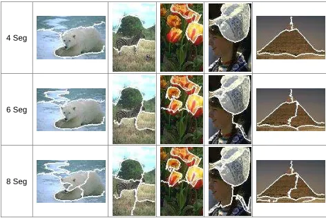
There are very many different automatic image segmen-tation algorithms. In this work the Normalized Cuts frame-work [13] is used, following the choice of [12], because it handles segmentation in a global way which has more chance than some approaches to segment out whole objects. In or-der to produce multiple segmentations, we varied one pa-rameter of the algorithm, namely the number of segments
K. Figure 1 shows some examples of segmented images at different levels of segmentation (K= 4,6 and 8). Evidently, some objects (polar bear, pyramid) get better segmentation at a low level (i.e. a small number of segments), while oth-ers (zebra, flower) do so at a high level. However, almost all the object get reasonably good segmentation at one of the levels, although not at the same one.
4 Seg
6 Seg
[image:2.595.318.554.245.403.2]8 Seg
Figure 1: Examples of segmented images at different levels of segmentation
2.2
Incorporating Training Image Based
Fea-ture Mapping with Multiple Segmentation
Previous work has shown the effectiveness of a training image based feature mapping in finding representative re-gions for labels [16], as well as in region based image auto-annotation [14]. However, in both cases a single level of seg-mentation is used. In this work, we incorporate the image-based feature mapping approach with the idea of multiple segmentations, in order to take into consideration the fact that different objects have their best segmentation at differ-ent levels. The details of the modified mapping algorithm is unfolded in the following.We denote training images asIi (i= 1,2, ...N, N being
the total number of images), and the jth segment in im-age Ii at the kth segmentation level asIikj. For the sake
of convenience, we line up all the segments from all the seg-mentation levels of the whole set of training images together and re-index them as It ( t = 1,2, ..., n, nbeing the total number of segments). In addition, we denote the vocabulary of the training set asWl(l= 1,2, ..., M,M being the total
number of keywords).
the training set. The coordinate of a label on a particular dimension is decided by the image this dimension represents. If the image is annotated by that label, the coordinate is 1, otherwise it is 0. Specifically, the mapping of word can be defined as
m(Wl) = [e(Wl, I1), e(Wl, I2), ..., e(Wl, IN)] (1)
wheree(Wl, Ii) indicates whether wordWlexists in training
imageIi, which can be further defined as
e(Wl, Ii) =
1 if image Iiis annotated with Wl
0 otherwise (2)
On the other hand, the coordinates of a segmentIt inF
are defined as:
m(It) = [d(It, I1), d(It, I2), ..., d(It, IN)] (3)
where d(It, I
i) represents the coordinate of segment It on
the ith dimension, which is either 1 or 0 according to the distance ofItto imageI
i. The distance of a segment to an
image is defined as the distance to the closest segment within all the segmentation levels of the image. By comparing seg-ments from all levels, we hope that good segseg-ments from different segmentations can be matched, which is less likely when single segmentation is used. The distance between two vectors/histograms V1 andV2, which represent the feature
descriptors of two segments, is measured by the normalised scalar product (cosine of angle), cos(V1, V2) = |V1•V2
V1||V2|. A
thresholdtis set to decide if two segments are close enough or not, which then generates either 1 or 0 as the coordinate on one dimension of the space. Mathematically it is defined as follows
d(It, Ii) =
1 if maxk=1,...,m(maxj=1,...,nik(cos(I
t, I
ikj)))> t
0 otherwise
(4) where m is the number of segmentation levels, nik is the
number of segments of image Ii at level k. The mapping
of segments can be comprehended as a mapping in which if the object that a segment contains also appears in a partic-ular training image, the coordinate of the segment on the dimension represented by that image is 1, otherwise 0.
We also choose normalised scalar product as the distance measure in space F. Intuitively, segments relating to the same objects or concepts should be close to each other in the feature space. In other words, if inFthe distance of two seg-mentsIxandIy, which is calculated ascos(m(Ix),m(Iy)),
is very small, they are very likely to contain the same object. Moreover, a label should be close to the image segments associated with the objects the label represents. Suppose the label is Wl, its distance to segments is computed as
cos(m(Wl),m(It)).
2.3
Application to Region-Based Image
Anno-tation
To annotate test images, all the test segments from all lev-els are mapped into the training image based feature space. The test set is denoted asTi0 (i0= 1,2, ...N0, N0 being the
total number of test images), and the j0th segment from the k0th level of image Ti0 is denoted as Ti0k0j0. All the
test segments are lined up and denoted asTt0. By applying the mappingm to a test segmentTt0, we can calculate its
coordinates in the training image based space as follows
m(Tt0) = [d(Tt0, I1), d(Tt
0
, I2), ..., d(Tt
0
, IN)] (5)
Region based image annotation becomes relatively straight-forward once the mapping is done. The probability of a segment being correctly annotated by a particular label, is approximated by their distance in the space. Furthermore, the probability of a test image being correctly annotated by a label, P(Wl, Ti0), is estimated by the highest probability
of this label being correct with any of the segments in that image, as follows
P(Wl, Ti0) =
maxk0=1,...,m0(maxj0=1,...,ni0k0(cos(m(Wl),m(Ti0k0j0))))
(6) where m0 is the number segmentation levels, while ni0k0 is
the number of segments of test imageTi0 at levelk0. Finally,
words with highest value of P(Wl, Ti0) are chosen as the
predicted captions of the image.
2.4
Key Features of the Algorithm
This mapping is similar to the work of [2], in which a region-based feature mapping is used. However, they de-fined a feature space in which each dimension is an image segment, and then map each image into the space. In other words, the two mappings are essentially the inverse of each other. However, our approach has two main advantages. One is that it is able to map image labels into the feature space, which effectively turns the problem of relating words and regions into one of comparing distances. For [2]’s map-ping, there is no way to identify the coordinate of a label on each dimension of the feature space because labels are only attached on an image basis, rather than a region basis. The other is that our approach can be incorporated with multi-ple segmentations in a more straightforward way. Segments from different levels of segmentations can be mapped into the same space, without making changes to the structure or dimensionality. In contrast, this is not the case for [2]’s approach.
2.5
A Simple Example
In this section a simple example is presented to illustrate the major steps of our algorithm. To make the example more comprehensible and easier, only a single level of seg-mentation is used here. It is not difficult to transfer the algorithm to the situation of multiple segmentations. The main difference is just that more segments need to be taken into account and more distances need to be calculated.
Consider two annotated training imagesI1, I2and one
un-annotated test imageT1;I1 is labelled as “RED, GREEN”
and half of the image is red and the other half is green;
I2 is labelled as “GREEN, BLUE” and half is green and
the other half is blue; half of T1 is red and the other half
is blue. Assume the segmentation algorithm manages to separate the two colours in each image and segments them into halves in at least one of the segmentations, we will have four training segments, denoted asI1
, I2
, I3
andI4
, and two test segments, denoted asT1
andT2
as
I1
= (255,0,0);
I2
= (0,255,0);
I3 = (0,255,0);
I4
= (0,0,255);
T1
= (255,0,0);
T2
= (0,0,255);.
(7)
Then we need to map the test segments into the feature space, which is a two dimensional space in this case as there are two training images. By applying Equation 3, the coor-dinates of the test segments are as follows:
T1: [1,0];
T2
: [0,1]; (8)
In addition, the labels can also be mapped into the feature space to give:
RED: [1,0];
GREEN: [1,1];
BLU E: [0,1];
(9)
It can now be seen that in the feature space, the closest labels for the test segments (regional label predictions) are:
T1
: RED;
T2: BLU E; (10)
3.
EXPERIMENT AND RESULTS
Previous work [14] has already demonstrated that the training image based feature space technique outperforms two other state of the art region based image auto-annotation techniques [5, 17]. Other image auto-annotation techniques were not considered because to the best of our knowledge, none of them is able to annotate image regions.
In this work, we compare the effectiveness of using mul-tiple segmentations for image auto-annotation with that of single segmentation. The same image collection1
, which was used in previous work [5, 17, 16], is adopted for the experi-ment. The dataset contains 5000 images from 50 Corel Stock Photo CDs, and has been divided into a training set of 4500 images and a test of 500 images. Each image had been anno-tated manually with 1-5 keywords. We used Normalised Cut [13] and varied the parameter of segment number to generate multiple segmentations for each image. In this work, three levels of segmentation are set, 4, 6 and 8. Therefore, the ap-proaches we are comparing are one multiple segmentation approach (denoted as Multi-Seg), which includes three lev-els 4, 6 and 8, and three single segmentation ones (denoted as 4-Seg, 6-Seg and 8-Seg).
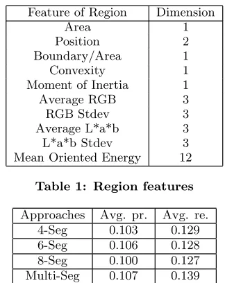
We follow [5]’s representation of regions, which is a 30 dimensional feature vector, including region average colour, size, location, average orientation energy and so on, as de-tailed in Table 1. Feature vectors are normalised to Z-Scores for distance measure in the image based space. Specifi-cally, suppose the whole set of training feature vectors are
V1, V2, ..., Vn,nbeing the total number of training image
seg-ments, andVi={Vi1, Vi2, ..., Vi30}, we calculate the Z-Score
for thejth dimension of theith vector as follows
Zij =
Vij−mean(V1j, V2j, ..., Vnj)
standard deviation(V1j, V2j, ..., Vnj)
(11)
1
Available at: http://kobus.ca/research/data/eccv 2002/index.html
Feature of Region Dimension
Area 1
Position 2
Boundary/Area 1
Convexity 1
Moment of Inertia 1
Average RGB 3
RGB Stdev 3
Average L*a*b 3
L*a*b Stdev 3
[image:4.595.354.516.50.254.2]Mean Oriented Energy 12
Table 1: Region features Approaches Avg. pr. Avg. re.
4-Seg 0.103 0.129
6-Seg 0.106 0.128
8-Seg 0.100 0.127
[image:4.595.132.214.69.138.2]Multi-Seg 0.107 0.139
Table 2: Performance comparison of using multiple segmentations for image auto-annotation with single segmentation
Note that for multiple segmentations, mean and standard deviation are calculated over the feature vectors from all segmentation levels, while for single segmentation, they are calculated within each segmentation level. Feature vectors of the test set are also normalised, using the mean and stan-dard deviation of the training vectors.
In order to find the optimal value for thresholdtin Equa-tion (4) for each approach, 500 random images are taken out of the training set for evaluation, by training on the remain-ing 4000 images. Thresholds with the best performances are chosen for the actual auto-annotation experiment. For each test image, the top 5 labels with the highest values of probability are chosen, according to Equation (6).
0 10 20 30 40 50 60 70 80 90 100 0 .9 9 0 .9 8 0 .9 7 0 .9 6 0 .9 5 0 .9 4 0 .9 3 0 .9 2 0 .9 1 0 .9 0 .8 9 0 .8 8 0 .8 7 0 .8 6 0 .8 5 0 .8 4 0 .8 3 0 .8 2 0 .8 1 0 .8 Multi Seg 4 6 8 Keyword Number with Recall>0
[image:5.595.158.453.57.227.2]Threshold
Figure 2: The number of keywords with recall>0 for each approach at different values of threshold
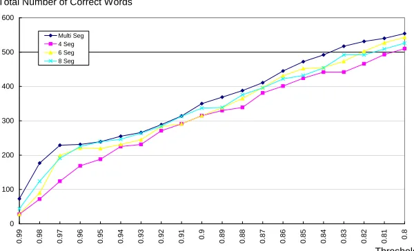
0 100 200 300 400 500 600 0 .9 9 0 .9 8 0 .9 7 0 .9 6 0 .9 5 0 .9 4 0 .9 3 0 .9 2 0 .9 1 0 .9 0 .8 9 0 .8 8 0 .8 7 0 .8 6 0 .8 5 0 .8 4 0 .8 3 0 .8 2 0 .8 1 0 .8 Multi Seg 4 Seg 6 Seg 8 Seg Threshold Total Number of Correct Words
Figure 3: The total number of correctly predicted words for each approach at different values of threshold
4.
CONCLUSIONS AND FUTURE WORK
A great number of automatic image annotation techniques use segmentation algorithms to partition the images before-hand. Generally, only one single level of segmentation is chosen, which is assumed to be correct. However, most of the segmentation algorithms do not give satisfying results at this time. We proposed a way of coupling multiple seg-mentations with image auto-annotation. The parameter of segmentation algorithm is varied to generate several levels of segmentation. On the other hand, a region based image annotation approach, namely the image based feature space, is utilized to incorporate with multiple segmentations. We have shown that annotation performance can be improved on a 5000 image collection when multiple segmentations are used.
As stated in [14], one current disadvantage of the approach is that the feature space has as many dimensions as training images in the set used to build the space. Ways in which the dimensionality of the space can be reduced without losing the association between segments, labels and images is being explored. In addition, the use of a different segmentation algorithm and feature descriptors is planned.
5.
REFERENCES
[1] K. Barnard, P. Duygulu, N. de Freitas, D. Forsyth, D. Blei, and M. I. Jordan. Matching words and pictures. Journal of Machine Learning Research, 3:1107–1135, 2003.
[2] J. Bi, Y. Chen, and J. Z. Wang. A sparse support vector machine approach to region-based image categorization. InCVPR ’05: Proceedings of the 2005 IEEE Computer Society Conference on Computer Vision and Pattern Recognition (CVPR’05) - Volume 1, pages 1121–1128, Washington, DC, USA, 2005. IEEE Computer Society.
[3] G. Carneiro and N. Vasconcelos. Formulating semantic image annotation as a supervised learning problem. In
CVPR (2), pages 163–168, 2005.
[4] Y. Deng, B. S.Manjunath, and H.Shin. Color image segmentation. InIEEE Computer Society Conference on Computer Vision and Pattern Recognition CVPR’99, volume 2, pages 446–451, Jun 1999. [5] P. Duygulu, K. Barnard, J. de Freitas, and D. Forsyth.
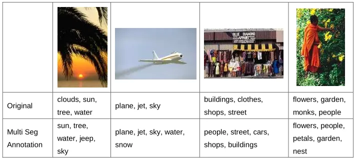
[image:5.595.154.454.261.443.2]Original clouds, sun,
tree, water plane, jet, sky
buildings, clothes,
shops, street
flowers, garden,
monks, people
Multi Seg
Annotation
sun, tree,
water, jeep,
sky
plane, jet, sky, water,
snow
people, street, cars,
shops, buildings
flowers, people,
petals, garden,
[image:6.595.127.484.52.210.2]nest
Figure 4: Some annotation examples by multiple segmentation based approach
European Conference on Computer Vision, pages IV:97–112, Copenhagen, Denmark, 2002.
[6] S. L. Feng, R. Manmatha, and V. Lavrenko. Multiple bernoulli relevance models for image and video annotation. InProceedings of the International Conference on Pattern Recognition (CVPR 2004), volume 2, pages 1002–1009, 2004.
[7] J. S. Hare and P. H. Lewis. Saliency-based models of image content and their application to
auto-annotation by semantic propagation. In
Proceedings of Multimedia and the Semantic Web / European Semantic Web Conference 2005, 2005. [8] J. Jeon, V. Lavrenko, and R. Manmatha. Automatic
image annotation and retrieval using cross-media relevance models. InSIGIR ’03 Conference, pages 119–126, 2003.
[9] V. Lavrenko, R. Manmatha, and J. Jeon. A model for learning the semantics of pictures. InProceedings of the Seventeenth Annual Conference on Neural Information Processing Systems, volume 16, pages 553–560, 2003.
[10] O. Maron and T. Lozano-P´erez. A framework for multiple-instance learning. In M. I. Jordan, M. J. Kearns, and S. A. Solla, editors,Advances in Neural Information Processing Systems, volume 10. The MIT Press, 1998.
[11] F. Monay and D. Gatica-Perez. On image auto-annotation with latent space models. In
Proceedings of the eleventh ACM international conference on Multimedia, pages 275–278, 2003. [12] B. C. Russell, A. A. Efros, J. Sivic, W. T. Freeman,
and A. Zisserman. Using multiple segmentations to discover objects and their extent in image collections. InProceedings of CVPR, pages 1605–1614, June 2006. [13] J. Shi and J. Malik. Normalized cuts and image
segmentation.IEEE Transactions on Pattern Analysis and Machine Intelligence (PAMI), pages 888–905, 2000.
[14] J. Tang and P. H. Lewis. Region based image annotation through a training image based feature space. Submitted to2007 International Conference on Image Processing (ICIP).
[15] J. Tang and P. H. Lewis. Image auto-annotation using
‘easy’ and ‘more challenging’ training sets. In
Proceedings of 7th International Workshop on Image Analysis for Multimedia Interactive Services, pages 121–124, 2006.
[16] J. Tang and P. H. Lewis. An image based feature space and mapping for linking regions and words. In
Proceedings of 2nd International Conference on Computer Vision Theory and Applications (VISAPP), Barcelona, Spain, 2007. Accepted.