Kernel classifier construction using orthogonal forward selection and boosting with Fisher ratio class separability measure

Kernel Classifier Construction Using Orthogonal Forward Selection and Boosting With Fisher

Ratio Class Separability Measure

S. Chen, X. X. Wang, X. Hong, and C. J. Harris

Abstract—A greedy technique is proposed to construct parsimonious kernel classifiers using the orthogonal forward selection method and boosting based on Fisher ratio for class separability measure. Unlike most kernel classification methods, which restrict kernel means to the training input data and use a fixed common variance for all the kernel terms, the proposed technique can tune both the mean vector and diagonal covariance matrix of individual kernel by incrementally maximizing Fisher ratio for class separability measure. An efficient weighted optimization method is developed based on boosting to append kernels one by one in an orthogonal forward selection procedure. Experimental results obtained using this construction technique demonstrate that it offers a viable alternative to the existing state-of-the-art kernel modeling methods for constructing sparse Gaussian radial basis function network classifiers that generalize well.

Index Terms—Boosting, classification, Fisher ratio of class separability, forward selection, kernel classifier, orthogonal least square, radial basis function network.

I. INTRODUCTION

A fundamental principle in practical nonlinear data modeling is the parsimonious principle of ensuring the smallest possible model that ex-plains the training data. Recently, the state-of-the-art kernel modeling techniques, such as the support vector machine (SVM) and relevant vector machine (RVM) [1]–[3], have widely been adopted in classifi-cation appliclassifi-cations to construct sparse classifiers that generalize well. Alternatively, a greedy technique can be applied to construct parsimo-nious classifiers by incrementally maximizing Fisher ratio of class sep-arability measure in an orthogonal forward selection (OFS) procedure [4], [5]. In most of the existing sparse kernel construction techniques, a fixed common variance is used for all the kernels and the kernel centers or means are placed at the training input data.

We present a flexible construction method for parsimonious clas-sifier modeling. The proposed algorithm tunes both the mean vector and diagonal covariance matrix of individual kernel by incrementally maximizing the Fisher ratio of class separability measure in an OFS procedure. To incrementally append the classifier’s kernels one by one, a weighted optimization search algorithm is developed, which is based on the idea from boosting [6]–[8]. Because kernel means are not restricted to the training input data and each kernel term has an individually tuned diagonal covariance matrix, our method can produce very sparse classifiers. The proposed weighted optimization algorithm is simple, robust, and easy to implement. Experimental re-sults are included to demonstrate the effectiveness of this incremental OFS construction algorithm with boosting (OFSwB) optimization for constructing Gaussian radial basis function network classifiers.

Manuscript received March 24, 2005; accepted February 10, 2006. S. Chen and C. J. Harris are with the School of Electronics and Computer Science, University of Southampton, Southampton SO17 1BJ, U.K. (e-mail: [email protected]; [email protected]).

X. X. Wang is with the Institute of Human Genetics, University of Newcastle, Newcastle upon Tyne NE1 3BZ, U.K. (e-mail: [email protected]).

X. Hong is with the Department of Cybernetics, University of Reading, Reading RG6 6AY, U.K. (e-mail: [email protected]).

Digital Object Identifier 10.1109/TNN.2006.881487

II. ORTHOGONALFORWARDSELECTION FOR CLASSIFIERCONSTRUCTION Consider the kernel classifier of the form

^cl= sgn(yl) with yl= M

i=1

wigi(xl) (1)

wherexlis anm-dimensional pattern vector with its associated class labelc_l 2 f61g; y_l is the classifier output for inputx_l, and^c_lis the estimated class label forxl; wi; 1 i M, denote the classifier weights,M is the number of kernels, andgi( 1 ); 1 i M, denote the classifier kernels. We allow the kernel function to be chosen as the general Gaussian functiongi(x) = G(x; i; 6i)with

G(x; _i; 6i) = exp 0 1₂(x 0 i)T601i (x 0 i) (2)

where the diagonal covariance matrix has the form of 6_i = diagf2_i;1; . . . ; _i;m2 g. Obviously, our method is equally applicable to other kernel functions. We will adopt an OFS procedure to build up the classifier (1) by appending kernels one by one.

Given theNpairs of training datafx_l; c_lgN_l=1, let us define the mod-eling residual asel = cl 0 yl. Then the classifier model(1) over the training data set can be expressed as

c = Gw + e (3)

wherec = [c1c21 1 1 cN]T; e = [e1e21 1 1 eN]T, the kernel matrix

G = [g1g21 1 1 gM] (4)

withg_k = [g_k(x1)gk(x2) 1 1 1 gk(xN)]T, and the classifier weight vectorw = [w₁w₂1 1 1 w_M]T. Let an orthogonal decomposition ofG be

G = PA (5)

where

A =

1 a1;2 1 1 1 a1;M

0 1 . .. ... ..

. . .. . .. _aM01;M

0 1 1 1 0 1

(6)

and

P = [p1p21 1 1 pM] =

p1;1 p1;2 1 1 1 p1;M

p2;1 p2;2 1 1 1 p2;M

..

. ... ... ... pN;1 pN;2 1 1 1 pN;M

(7)

with orthogonal columns that satisfypT_ipj = 0, ifi 6= j. The model (3) can alternatively be expressed as

c = P + e (8)

where the weight vector = [121 1 1 M]T for the orthogonal model satisfies the triangular systemAw = .

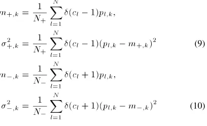
A sparsek-term classifier model can be selected by incrementally maximizing a class separability measure in an OFS procedure [4], [5]. Define the two class setsC6= fxl: cl= 61g, and let the numbers of points inC6beN6, respectively, withN++N0= N. The means and

variances of training samples belonging to classesC₆in the direction of basispkare given by

m+;k= 1_N +

N

l=1

(cl0 1)pl;k;

2 +;k= 1_N

+ N

l=1

(cl0 1)(pl;k0 m+;k)2 (9)

m0;k= 1_N 0

N

l=1

(cl+ 1)pl;k;

2 0;k= 1_N

0 N

l=1

(cl+ 1)(pl;k0 m0;k)2 (10)

respectively, where(x) = 1forx = 0and(x) = 0forx 6= 0. Fisher ratio,1_{defined as the ratio of the interclass difference and the} intraclass spread, in the direction ofp_kis given by [9]

Fk= (m+;k0 m0;k) 2

2

+;k+ 20;k :

(11)

At thekth stage of incremental modeling, thekth term is selected to maximize the Fisher ratio (11). However, unlike the original OFS pro-cedure [4], [5], which restricts the choice of the kernel center_kto the training data points and uses a fixed common variance, the maxi-mization here is with respect to the mean vector_k and the diagonal covariance matrix6k of thekth kernel term. The forward selection procedure is terminated at thekth stage if

Fk k i=1Fi

< (12)

is satisfied, where the small positive scalaris a chosen tolerance that determines the sparsity of the selected classifier model. The appropriate value foris problem dependent and has to be found empirically. Alter-natively, cross-validation can be employed to terminate the OFS proce-dure. The least square solution for the corresponding sparse classifier weight vectorw_kis readily available given the least square solution ofk.

III. WEIGHTEDOPTIMIZATIONWITHBOOSTING

It can be seen that at each incremental modeling stage, the basic task is to maximize the Fisher ratio criterionFk(u)overu 2 U, where the vectorucontains the kernel mean vectorand the diagonal co-variance matrix6. This task may be carried out by some global opti-mization methods, such as the genetic algorithm [10], [11] and adap-tive simulated annealing [12], [13]. These standard global optimization methods are, however, computationally very expensive. Let us consider a simple search method to perform this optimization. Givenspoints of u; uifor1 i s, letubest = arg maxfFk(ui); 1 i sgand uworst = arg minfFk(ui); 1 i sg. An (s+1)th pointus+1is

first generated by a weighted convex combination ofui; 1 i s. An (s+2)th valueu_s+2is then generated as the mirror image ofu_s+1, with respect toubest, along the direction defined by ubest0 us+1. The best ofus+1 andus+2then replacesuworst. The process is re-peated until it converges. A simple illustration is depicted in Fig. 1 for a one-dimensional case, where there ares = 3points,u1; u2andu3, andu_best= u₂andu_worst= u₃. The fourth valueu₄is a weighted combination ofu1; u2;andu3, andu5is the mirror image ofu4with respect tou₂. Asu₄is better thanu₅, it will replaceu₃.

1_{In this paper, we restrict to the two-class classification problem. The}

defi-nition of Fisher ratio, however, is applicable to the multiclass case, and the al-gorithm presented in this paper can be extended to the multiclass classification problem. Also see [4].

Fig. 1. Illustration of a simple weighted search optimization process.

Fig. 2. Synthetic data: training and test error rates versus size of selected clas-sifier.

Clearly, how the weighted combination is performed is crucial. The weightings foru_i; 1 i s, should reflect the “goodness” ofu_iand, moreover, the process should be capable of self-learning or adapting these weightings. This is exactly the basic idea of boosting [6]–[8]. Specifically, we combine the AdaBoost algorithm of [6] with the afore-mentioned simple search strategy to form a weighted search routine. This weighted search routine performs a guided random search with a population ofsmembersui; 1 i s, and the solution obtained may depend on the initial choice of population. To derive a robust algo-rithm that is independent of the initial choices of population and to im-prove the probability of achieving a global optimal solution, we adopt a strategy of repeating the weighted search routine with an elitist ini-tialization of the population, namely, each repeat or generation of the weighted search will start by retaining the solution found in the pre-vious generation and filling the rest of the population randomly. The resulting weighted optimization algorithm, referred to as the OFSwB, is summarized as follows, given the training datafx_l; c_lgN_l=1at thekth stage of modeling.

A. Outer Loop: Number of Generations—l = 1 : Lmax

1) Initialization:

a) Setu1 = u(l01)best and randomly generate the rest of the

popula-tion membersui; 2 i s, whereu(l01)_best denotes the solution found in the previous generation. Ifl 0 1 = 0; u₁is also ran-domly chosen.

b) Set the inner loop iteration indext = 0and the initial weightings d(t)

i = (1=s)for1 i s.

c) For1 i s, generateg(i)_k fromui, thescandidates for the kth model column, and orthogonalize them

(i)_j;k=pTjg(i)k

pT

jpj for 1 j < k

p(i)

k = gk(i)0 k01

j=1

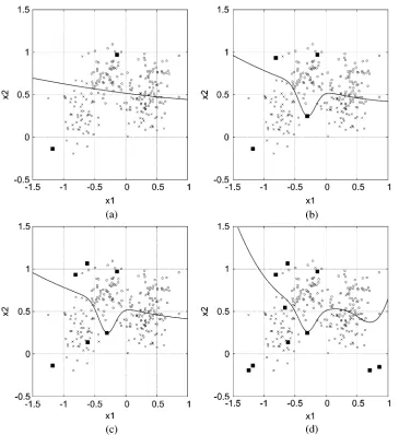
Fig. 3. Synthetic data: (a) decision boundary of the two-term classifier, (b) decision boundary of the four-term classifier, (c) decision boundary of the six-term classifier, and (d) decision boundary of the ten-term classifier. The 250 samples of the training data are shown as crosses and circles for the two classes, respectively, and the kernel centers are depicted by the dark-filled squares.

d) For1 i s, calculate the loss of each point, namely

J_k(i)= 1 F_k(i)

whereF_k(i)denotes the Fisher ratio (11) calculated in the direc-tion ofp(i)_k .

B. Inner Loop: Weighted Search Routine

Step 1) Boosting. 1) Find

ubest= arg minfJk(i); 1 i sg

uworst= arg maxfJk(i); 1 i sg:

2) Normalize the loss

J_k(i)= Jk(i) s l=1Jk(l)

; 1 i s:

3) Compute a weighting factor_taccording to

t=_{1 0} t

t with t= s

i=1

d(t) i Jk(i):

4) Update the weighting vector

d(t+1)i = d (t) i

J

t fort 1

d(t)

i t10J fort> 1;

1 i s:

5) Normalize the weighting vector

d(t+1)_i = d(t+1)i s l=1dl(t+1)

; 1 i s:

Step 2) Parameter updating.

1) Construct the (s+1)th point using the formula

us+1= s

i=1

d(t+1)i ui:

2) Construct the (s+2)th point using the formula

us+2= ubest+ (ubest0 us+1):

3) Orthogonalize these two candidate model columns and compute their losses.

4) Choose a better (smaller loss value) point fromus+1

TABLE I

OFS PROCEDUREWITHBOOSTING FOR THESYNTHETICDATASET

Repeat from Step 1) witht = t + 1until the (s+1)th value changes very little compared with the last round or a preset maximum number of iterations has been reached.

C. End of Inner Loop

From the converged population ofspoints, find

ik= arg minfJ_k(i); 1 i sg

and select_j;k = (i )_j;k ; 1 j < kand

pk= p(i )k = g(i )k 0 k01

j=1

j;kpj:

This determines the solution of thelth generation, denoted asu(l)_best. Repeat from outer loop untill = L_max.

D. End of Outer Loop

This determines thekth kernel’s mean vector and diagonal covari-ance matrix or selects thekth kernel term.

The important algorithmic parameters that need to be chosen appro-priately are the population sizesand the number of generationsLmax. The population size depends on the dimension ofuand the objective function to be optimized. This is very similar to the choice of popula-tion size in the genetic algorithm. The number of generapopula-tions should be chosen sufficiently large for the algorithm to search for a global min-imum but not too large, which may incur unnecessary computation. Again, the appropriate value forL_maxdepends on the dimension ofu and how hard is the objective function to be optimized. Also the choice ofshas some influence on the choice ofL_max. Generally, these two algorithmic parameters have to be found empirically.

IV. EXPERIMENTALRESULTS

The synthetic two-class problem and Diabetes in Pima Indians, taken from [14], were used to investigate the proposed OFSwB algorithm.2

A. Synthetic Data

The dimension of the feature space wasm = 2. The training set contained 250 samples and the test set had 1000 points. The optimal Bayes error rate for this example is around 8%. With a population size s = 21and the number of generationsLmax = 20, we applied the OFSwB algorithm to the 250-sample training set. Fig. 2 depicts the training and test error rates versus the size of the selected classifier. The decision boundaries of the two-term, four-term, six-term, and ten-term classifiers are illustrated in Fig. 3(a)–(d), respectively. The decision boundary of the eight-term classifier, not shown here, is almost iden-tical to that of the four-term classifier. The result of Fig. 2 indicates that the four-term classifier is sufficient, and the selection procedure for this four-term classifier is summarized in Table I. Note that the four-term classifier constructed by the OFSwB algorithm achieved the optimal

2_{The data sets were obtained from http://www.stats.ox.ac.uk/PRNN/}

TABLE II

COMPARISON OFCLASSIFICATION FOR THESYNTHETICDATASET

Fig. 4. Pima Diabetes data: training and test error rates versus size of selected classifier.

TABLE III

COMPARISON OFCLASSIFICATION FOR THEPIMADIABETESDATASET

Bayes classification performance. Tipping [3] applied the SVM and RVM to this data set and only used 100 random selected samples from the 250-points training data set in training. The results given in [3] are compared with our result in Table II.

B. Pima Diabetes Data

The dimension of the input space wasm = 7, the training data set contained 200 samples and the test data set had 332 samples. With a population sizes = 61and the number of generationsLmax = 20

for the OFSwB algorithm, Fig. 4 shows the training and test error rates versus the size of the selected classifier, which clearly indicates that a four-term classifier is sufficient. Table III compares the performance of the selected four-term classifier with those obtained by the SVM and RVM methods, quoted from [3].

V. CONCLUSION

search method has been developed based on boosting to append classi-fier kernels one by one in an orthogonal forward regression procedure. Experimental results presented have demonstrated the effectiveness of the proposed technique.

REFERENCES

[1] V. Vapnik, The Nature of Statistical Learning Theory. New York: Springer-Verlag, 1995.

[2] B. Schölkopf and A. J. Smola, Learning with Kernels: Support Vector Machines, Regularization, Optimization, and Beyond. Cambridge, MA: MIT Press, 2002.

[3] M. E. Tipping, “Sparse Bayesian learning and the relevance vector ma-chine,”J. Machine Learn. Res., vol. 1, pp. 211–244, 2001.

[4] K. Z. Mao, “RBF neural network center selection based on Fisher ratio class separability measure,”IEEE Trans. Neural Netw., vol. 13, no. 5, pp. 1211–1217, 2002.

[5] S. Chen, L. Hanzo, and A. Wolfgang, “Kernel-based nonlinear beam-forming construction using orthogonal forward selection with Fisher ratio class separability measure,”IEEE Signal Process. Lett., vol. 11, no. 5, pp. 478–481, 2004.

[6] Y. Freund and R. E. Schapire, “A decision-theoretic generalization of on-line learning and an application to boosting,”J. Comput. Syst. Sci., vol. 55, no. 1, pp. 119–139, 1997.

[7] R. E. Schapire, “The strength of weak learnability,”Machine Learn., vol. 5, no. 2, pp. 197–227, 1990.

[8] R. Meir and G. Rätsch, “An introduction to boosting and leveraging,” in

Advanced Lectures in Machine Learning, S. Mendelson and A. Smola, Eds. Berlin, Germany: Springer Verlag, 2003, pp. 119–184. [9] R. O. Duda and P. E. Hart, Pattern Classification and Scene Analysis.

New York: Wiley, 1973.

[10] D. E. Goldberg, Genetic Algorithms in Search, Optimization and Ma-chine Learning. Reading, MA: Addison Wesley, 1989.

[11] K. F. Man, K. S. Tang, and S. Kwong, Genetic Algorithms: Concepts and Design. London, U.K.: Springer-Verlag, 1998.

[12] L. Ingber, “Simulated annealing: Practice versus theory,” Math. Comput. Model., vol. 18, no. 11, pp. 29–57, 1993.

[13] S. Chen and B. L. Luk, “Adaptive simulated annealing for optimization in signal processing applications,”Signal Process., vol. 79, no. 1, pp. 117–128, 1999.

[14] B. D. Ripley, Pattern Recognition and Neural Networks. Cambridge, U.K.: Cambridge Univ. Press, 1996.

Self-Organizing Map Algorithm Without Learning of Neighborhood Vectors

Hiroki Kusumoto and Yoshiyasu Takefuji

Abstract—In this letter, a new self-organizing map (SOM) algorithm with computational costO(log M)is proposed whereM is the size of a feature map. The first SOM algorithm withO(M )was originally proposed by Ko-honen. The proposed algorithm is composed of the subdividing method and the binary search method. The proposed algorithm does not need the neigh-borhood functions so that it eliminates the computational cost in learning of neighborhood vectors and the labor of adjusting the parameters of neigh-borhood functions. The effectiveness of the proposed algorithm was exam-ined by an analysis of codon frequencies ofEscherichia coli (E. coli)K12 genes. These drastic computational reduction and accessible application that requires no adjusting of the neighborhood function will be able to con-tribute to many scientific areas.

Index Terms—Binary search, computational reduction, codon fre-quency,Escherichia coli (E. coli), neighborhood function, self-organizing map (SOM), subdividing method.

I. INTRODUCTION

A self-organizing map (SOM) algorithm is one of unsupervised learning methods in the artificial neural network in order to map a multidimensional input data set into two-dimensional (2-D) space according to the neighborhood function. The first SOM algorithm was originally developed by Kohonen [1] and has been used in a variety of research areas including speech or speaker recognition [2], mathematics [3], financial analysis [4], color quantization [5], identification and control of dynamical systems [6], color clustering [7], and bioinformatics [8]–[10]. Particularly in the field of bioinfor-matics, many researchers have adopted SOM algorithm for analysis of gene sequences as a method of clustering, visualization, or feature extraction. Wanget al.clustered genes according to codon usage by SOM algorithm in order to identify highly expressed and horizon-tally transferred genes [8]. Sultanet al.and Gillet al.applied SOM algorithm to analyze microarray data [9], [10].

When M2 is the size of a feature map, the number of compared weight vectors for one input vector to search a winner vector by ex-haustive search is equivalent toM2. Tree-structured SOM proposed by Koikkalainen and Oja [11] and Truong [12] to improve the winner search reduces the number of searching operations toO(M log M). Kohonen proposed a new method with the total number of compar-ison operations byO(M)[1]. Self-organizing topological tree with O(log M)was proposed by Xu and Chang [13].

In this letter, a new SOM algorithm withO(log₂M) is proposed where it is composed of the subdividing method and the binary search method. The proposed algorithm not only reduces the computational costs but also eliminates the time-consuming parameter tuning in the neighborhood function in SOM applications. When we use SOM for practical analyses, one of the most time-consuming tasks for effective learning is to adjust the values of several parameters, particularly in neighborhood function. In addition to that, the neighborhood function has a critical effect on the performance of SOM. In the proposed algo-rithm, only winner vectors are trained. The proposed algorithm not to train neighborhood vectors is completely original.

Manuscript received May 4, 2005; revised April 3, 2006.

The authors are with the Keio University, Kanagawa 252-8520, Japan (e-mail: [email protected]).

Digital Object Identifier 10.1109/TNN.2006.882370