Devolatilization During the Formation of Rocky Planets: Bulk Elemental Composition

(1)

Devolatilization During the Formation of Rocky

Planets: Bulk Elemental Composition

Haiyang Wang

A thesis submitted for the degree of

Doctor of Philosophy

of The Australian National University

Research School of Astronomy and Astrophysics College of Science

The Australian National University Canberra ACT 2611, Australia

(2)

Composition"

(3)

Dedicated to my parents

献给我的父母亲

"Home is a name, a word, it is a strong one; stronger than magician ever spoke,

(4)

(5)

Declaration

This thesis is an account of my research undertaken between February 2014 and March 2018 at the Research School of Astronomy and Astrophysics, College of Sci-ence, the Australian National University. The material presented in this thesis is original, and has not been submitted in whole or part for a degree in any university.

This thesis is based on four papers that I published or submitted during my PhD research. I have made significant contributions to each paper. Below I describe my contributions to the research in each chapter and associated paper.

1. Chapter 1 is completely written by me. Section 1.2 is adapted from the publi-cation Wang and Lineweaver [2016] where all the research is my work. It was written by me with comments from my coauthor.

2. Chapter 2 is adapted from Wang et al. [2018a] originally published in Icarus 299, 460-474. I conducted all the analysis and wrote the full paper collabora-tively with my coauthors.

3. Chapter 3 is under review/Icarus as Wang et al. [2018b]. I conducted all the analysis and wrote the full paper collaboratively with my coauthors.

4. Chapter 4 is adapted from Wang et al. [2019] originally published in MNRAS 482, 2222-2233. I conducted all the analysis, wrote the full paper and finalized it with comments from my coauthors.

5. Chapter 5 is summarized by me from the previous chapters. The first part of the ‘Future Work’ is summarized from a manuscript in preparation by me, Charles H. Lineweaver, Trevor R. Ireland, and others. The future directions are independently written by me.

Haiyang Wang 30 November 2018

(6)

(7)

Acknowledgments

This thesis is being wrapped up ten years since I completed the dissertation for my first degree. Following the conferral of my second degree six years ago, I was deter-mined to transition from being an exploration geophysicist to being an astronomer specializing in extrasolar planets and extraterrestrial habitability. Before I acknowl-edge the people who supported me on this new journey, I would like to thank my old friends and colleagues, who offered their help, support, and encouragement, en-abling me to begin this adventure. There are too many of you to mention by name, but I thank you all from the bottom of my heart. I would also like to thank the Australian Government Department of Education and Training for awarding me the Prime Minister’s Australia Asia Endeavour Scholarship, without which I would have never embarked on this journey.

For my PhD research, I would like to first express my gratitude to my primary su-pervisor, Charley Lineweaver, for his patient guidance, critical comments, and sharp insights. Your enthusiasm for science, breadth of knowledge, and articulation of thoughts is inspiring. The opportunity to work with you is sincerely appreciated, and the experience has been rewarding for me.

I would also like to thank Trevor Ireland, for his time and the insights he brought into all our discussions. His advice on both my PhD and career development is par-ticularly appreciated. Thank you David Yong for your unwavering support during the late stages of my PhD as well as always being available to answer my many (of-ten naive) questions. Mark Krumholz (my panel chair) and Gary Da Costa (school graduate convener) were invaluable in helping me sort out several administrative roadblocks that I encountered during my PhD. Thanks to Marc Norman for his con-tinued support, encouragement, and interest in my work.

I have also benefited from discussions with other researchers such as Martin As-plund, Brent Groves, Mike Ireland, and Joao Bento from the Research School of Astronomy and Astrophysics (RSAA) as well as Yuri Amelin, Hrvoje Tkalˇaci´c, Pene-lope King, and Hugh O’Neil from the Research School of Earth Sciences. I would like to acknowledge the travel support from both ANU and RSAA, which enabled me to travel to conferences and research institutes where I met and talked to many distinguished scholars including William F. McDonough, Ramon Brasser, Steve Mo-jzsis, Stephen Kane, Brad Carter, and Jane MacAuthor. The discussions with them have broadened my vision, enhanced my research, and inspired me to advance.

I feel very fortunate to be surrounded by a range of amazing peers throughout my graduate study at Mount Stromlo. I would like to firstly thank Aditya Chopra, my mentor and friend, for his advice whenever I felt stressed or disoriented. I would also like to specially thank Suryashree Aniyan and Thomas Nordlander, for their

(8)

Acharyya, Soniya Sharma, Adam Rains, and many others, thank you all for having stood by me through my ups and downs at Mount Stromlo.

I am perpetually indebted to my parents, for their patience, support, and belief in me throughout my life. And to my sisters and brother, thank you for having spent more time with our parents during my absence.

(9)

Abstract

As the solar nebula condensed, evaporated and fractionated to form the nascent Earth, the bulk elemental composition of the Earth was established. To first order, the Earth is a devolatilized sample of the solar nebula. Similarly, rocky exoplanets are also likely devolatilized samples of the stellar nebulae out of which they and their host stars formed. If this assumption holds, we can estimate the chemical composition of rocky exoplanets by applying a devolatilization algorithm based on the elemental abundances of their host stars. This thesis is an investigation of this potentially universal devolatilization pattern, from which exoplanetary chemistry and habitability are then derived.

To quantify (in broad terms) the chemical relationships between the Earth, the Sun and other bodies in the Solar System, the elemental abundances of the bulk Earth are required. The key to comparing Earth’s composition with those of other objects is to have a determination of the bulk composition with an appropriate estimate of un-certainties. We present concordance estimates (with uncertainties) of the elemental abundances of the bulk Earth, by compiling, combining, and renormalizing a large set of heterogeneous literature values of the primitive mantle and of the core. The weighting factor for the concordance estimates comes from our new estimate of the core mass fraction of the Earth: 32.5±0.3 wt% (weight percent). The uncertainties on our elemental abundances usefully calibrate the unresolved discrepancies between standard Earth models made under various geochemical and geophysical assump-tions.

We then extend our assessment of terrestrial abundances to the modeling of pro-tosolar abundances based on the latest estimates of solar photospheric abundances and primitive meteoritic abundances. We compare our new protosolar abundances with our estimates of bulk Earth composition, thereby quantifying the devolatiliza-tion of the solar nebula that led to the formadevolatiliza-tion of the Earth. As a funcdevolatiliza-tion of elemental 50% condensation temperatures (TC), we fit the Earth-to-Sun abundance ratios f to the linear trend log(f) = alog(TC) +b. The best fit coefficients are:

a=3.676_±0.142 andb= 11.556_±0.436. The quantification of the slopeaprovides

an empirical observation upon which modeling of the devolatilization processes can be based. These coefficients determine a critical devolatilization temperature for the Earth TD(E) = 1391±15 K. The resultant devolatilization pattern allows inferences

to be made concerning the depletions of elements in the early solar system and is potentially useful for estimating the chemical composition of rocky exoplanets from their known host stellar abundances.

We apply the devolatilization pattern to nearby planetary systems to infer the bulk elemental composition of rocky exoplanets – particularly those within the cir-cumstellar habitable zones – from the known host stellar elemental abundances. The

(10)

(11)

List of Figures

1 . . . i

1.1 From the proto-Sun to the planet Earth . . . 7

1.2 The terrestrial volatility trend . . . 8

1.3 Solar System abundances in the literature . . . 10

1.4 Chemical complementarity between the ISM gas phase and the solar system rocky material . . . 12

1.5 Inheritance processes from the ISM to the protoplanetary disk . . . 13

1.6 Observational information required for modeling exoplanetary chem-istry and interiors . . . 15

1.7 Comparison of normalized elemental abundances between a variety of solar system rocky bodies . . . 16

2.1 Concordance estimates (with uncertainties) of the primitive mantle (PM) composition of the Earth . . . 24

2.2 Zoom-in of the estimates of the 13 most abundant elements in the PM . 25 2.3 Concordance estimates (with uncertainties) of the core composition of the Earth . . . 32

2.4 Zoom-in of the estimates of the 13 most abundant elements in the core 33 2.5 The concordance PM and core_!the concordance bulk Earth . . . 35

2.6 The elemental abundances (with uncertainties) of bulk Earth . . . 36

2.7 Zoom-in of the 15 most abunant elements in bulk Earth . . . 37

2.8 On the normalization of the PM and bulk Earth elemental abundances to CI chondritic abundances . . . 39

3.1 Similarity of meteoritic and photospheric abundances . . . 47

3.2 Estimates of protosolar abundances from photospheric and CI chon-dritic data . . . 50

3.3 Protosolar mass fractions of H (X), He (Y) and metals (Z) . . . 54

3.4 On the normalization of elemental abundances of bulk Earth to proto-Sun . . . 56

3.5 The devolatilization pattern from the solar nebula to the planet Earth . 57 3.6 Comparison of the devolatilization pattern with the previous volatility trends . . . 58

3.7 Extrapolation of the devolatilization pattern to the realm of highly volatile elements . . . 61

3.8 Devolatilization from the solar nebula to CI chondrites . . . 64

3.9 From the solar nebula to rocky bodies: devolatilization matters . . . 65

(16)

4.1 Devolatilization patterns from stellar nebulae to terrestrial exoplanets . 73 4.2 Distribution of Fe/Ni ratios of more than 4900 FGK-type stars within

150 pc of the Sun . . . 76 4.3 Computational procedure scheme of elemental fractionation . . . 78 4.4 The comparison of key elemental ratios between Kepler-10 and its

po-tential exo-Earth . . . 81 4.5 The comparison of key elemental ratios between the potential

exo-Earths respectively orbiting 10, 20, 21, and Kepler-100 . . . 82 4.6 (a) A ternary diagram illustrating the estimates of the mantle

compo-sition; (b) A bar graph comparing the estimates of the core molar mass fraction of these exo-Earths . . . 85

5.1 The elemental abundances (relative to hydrogen) ofaCen A & B . . . . 93

5.2 The elemental abundances of potential terrestrial planets in the habit-able zones of theaCen AB system . . . 94

(17)

List of Tables

2.1 Concordance estimates of the elemental abundances of primitive man-tle, core, and bulk Earth . . . 27 2.2 Concentrations of the 13 most abundant elements in the core . . . 30 2.3 Core mass fraction in the Earth . . . 34

3.1 The combination approach of photospheric and meteoritic abundances 48 3.2 Estimates of protosolar abundances from photospheric and CI

chon-dritic data . . . 51 3.3 Protosolar mass fractions of H (X), He (Y) and metals (Z) . . . 54 3.4 Comparison of the parameters of the devolatilization pattern and the

previous volatility trends . . . 59 3.5 Fractional distribution of carbon and oxygen between volatile and

re-fractory phases in the solar nebular material . . . 62

4.1 Bulk elemental composition of potential habitable-zone terrestrial ex-oplanets (i.e. exo-Earths) around the studied host stars . . . 75 4.2 Comparison of the estimates of the interior compositions of the “model

Earth” with other independent estimates . . . 80 4.3 Estimates of the interior composition and structure of potential

exo-Earths . . . 83 4.4 Conservative estimates of the interior composition and structure of any

rocky exoplanet orbiting the studied planet host stars . . . 86

A.1 Significances of deviations between our concordance bulk Earth abun-dances and previous estimates . . . 127 A.2 Rescaling the sums of elemental abundances (ppm by mass) for Earth

components . . . 128

(18)

(19)

Chapter1

Introduction

Life is only known to exist on a single planet, the Earth. For life-forms like us, the most important feature of Earth is the fact that it is habitable – i.e. suitable for life over geological time-scales. Understanding habitability and using that knowledge to search for the nearest habitable planets may be crucial for our survival as a species in the far future [Lineweaver and Chopra, 2012; Sagan, 1994]. Aside from other rocky bodies in the solar system, exoplanet detection missions have discovered and con-firmed over 3700 planets1_{, which likely represent a small sample of many billions of}

planets yet-to-be found in our Galaxy. The discussion regarding what fraction of such planets could be Earth-like and even habitable to life as we know it is intensive [e.g. Kasting et al., 2014; Bovaird et al., 2015; Kane et al., 2016; Chopra and Lineweaver, 2016; Kaltenegger, 2017]. The near-future telescopes (e.g. JWST, WFIRST, LUVOIR, GMT and ELT) will herald a new era of space-based and ground-based observations capable of characterizing close-by habitable worlds like our own.

The principal planetary characteristics that govern the potential of a planet to host a biosphere are aspects such as mass, radius, and orbital parameters (“phys-ical characteristics”) and the composition of the atmosphere, surface, and interior (“chemical characteristics”) [Meadows et al., 2009; Hinkel and Unterborn, 2018]. The physical characteristics of a planet, in addition to the planet’s incident flux from its parent star, can determine whether it is located in the (circumstellar) habitable zone, which is usually defined as the region around a star where a planet can support liquid water on its surface given sufficient atmospheric pressure [e.g. Huang, 1959; Hart, 1979; Kasting et al., 1993; Lineweaver and Chopra, 2012; Kopparapu et al., 2013; Kane et al., 2016]. A more definitive determination of whether a planet can support liquid water and potentially harbor life on its surface requires the characterization of the planetary atmosphere [Meadows et al., 2009; Kasting et al., 2014] and, if possible, of the surface and interior.

Unlike the spectra of stars, the sensitivity of spectroscopic techniques to the spec-tra of exspec-trasolar planets is inadequate because of the much fainter luminosity of rocky planets compared with their host stars. Some successful attempts to derive the possible exoplanetary compositions from externally polluted white dwarfs have

1_{NASA Exoplanet Archive,} _{https://exoplanetarchive.ipac.caltech.edu}_{, accessed March 15,}

2018.

(20)

been reported in recent years [e.g. Klein et al., 2011; Zuckerman et al., 2011; Xu et al., 2014], but the observable types of exoplanets and the derivable number of elements are still limited.

Promising methods have been developed to directly measure the atmospheric composition of extrasolar planets by means of transmission spectroscopy [e.g. Char-bonneau et al., 2002; Swain et al., 2009; Kaltenegger, 2017]. This method is available for those extrasolar planets that eclipse their host star, so that the planetary atmo-sphere filters the starlight and the atmoatmo-sphere’s composition can thereby be mea-sured. However, an extrasolar planet’s atmospheric composition is not the same as its overall, bulk, composition. The bulk composition of extrasolar planets can be es-timated, for example, by combining planetary dynamical and chemical simulations [Bond et al., 2010a,b; Carter-Bond et al., 2012], or by assuming that compositional differences relative to exoplanet host stars are similar to those found between the Sun and other solar system bodies [Lineweaver and Robles, 2009].

The chemical composition of the Earth is in some respects remarkably similar to that of the Sun. This is especially true for the rock-forming elements, which are expected to have solidified early on during the formation of the planetary system. Volatile material (e.g. hydrogen, carbon, and oxygen) on the other hand is clearly deficient in Earth’s composition, and the mechanism that caused the volatile ele-ments to become deficient is called “devolatilization”. Understanding the physical processes accounting for the volatile depletion is a hot topic that has been debated for many decades. This debate initially focused on the origin and formation of chon-drites starting from late 1950s through 1960s [e.g. Urey, 1957, 1961, 1964, 1967; Wood, 1958, 1961, 1962, 1963, 1967; Ringwood, 1959, 1961, 1953, 1965, 1966; Mason, 1960a,b, 1963; Fish et al., 1960; Fish and Goles, 1962; Anders, 1960, 1963, 1964]. By now, a variety of models/hypotheses – often distinct and sometimes conflicting - have been proposed to explain the mechanisms of volatile depletion observed in various mete-orites and in planetary bodies. Which of these will prevail will depend heavily on our understandings of thermal histories in the early solar system (see 1.1.1 for further discussion).

A related question is, to what extent can these sampled solar system bodies be representative for the whole solar system and can the devolatilization processes in the Solar System be a template for those that occurred during the formation of other planetary systems. No one can answer this question precisely, due to our limited knowledge of a complete picture of the formation of the Solar System, let alone that of other planetary systems. However, using the samples that we have the most com-prehensive and accurate information of, investigating potential relationships/pat-terns between these samples should be a crucial step in understanding our planetary system and, by extension, in constraining the characterization of our neighborhood systems.

(21)

3

early solar system and is potentially useful for estimating the chemical composition of rocky exoplanets from the spectroscopic measurements of their host stars.

This chapter provides a background overview of the topics discussed in the thesis. Section 1.1 reviews the studies of the devolatilization from the solar nebula to the Earth, including the compositional estimates of the proto-Sun and bulk Earth.

Section 1.2 sets the context for the formation of the terrestrial planets, particularly from the perspective of chemical inheritance from the interstellar medium.

(22)

1 .

1 From the Solar Nebula to the Planet Earth:

Devolatiliza-tion Matters

1.1.1 A snapshot of volatile fractionation in the early solar system

Astrophysical modeling of the relatively high temperatures in the inner solar nebula (compared to the outer) [e.g. Dullemond et al., 2002; D’Alessio et al., 2006; Dullemond and Monnier, 2010; Salmeron and Ireland, 2012a], combined with observations that volatile fractionations in chondrites – the most common and primitive type of mete-orites – are mostly related to volatility in some way [e.g. O’D. Alexander, 2001; Bland et al., 2005; Davis, 2006; Braukmüller et al., 2018], lead to the picture of a vaporized early inner solar system.

Over the past 70 years, numerous models have been proposed to explain volatile fractionation in planetary materials. Anders [1964] reviewed the debate that started in the 1950s regarding the formation of chondrites. He advocated the Wood model [Wood, 1958, 1961, 1962, 1963] that was further developed by him to a two-component model. In this model, all chondrites accreted (i) a fine-grained, volatile-rich material called “matrix” and (ii) a coarse-grained, refractory fraction that formed at high tem-perature called “chondrules”. Melting and evaporative losses of volatiles during chondrule formation account for the observed carbonaceous chondrite fractionation [see Larimer and Anders, 1967; Alexander, 2005]. Localized heat sources – e.g. shock waves and massive lightning discharges [Connolly and Love, 1998; Desch and Cuzzi, 2000] – are thought to account for the evaporation [O’D. Alexander, 2001; Alexander, 2005].

However, this two-component model has been criticized by Palme and Boynton [1993] and Cassen [1996], based on the following arguments against it: (i) chondrules are, on average, too volatile rich, e.g. for Na and K [Rubin and Wasson, 1987; Spettel et al., 1989], and matrix is not sufficiently enriched in volatile elements as expected from this model; (ii) the fractionation patterns cannot be reproduced in experiments in which meteoritic material is evaporated [Bart et al., 1980; Wulf et al., 1995]; (iii) evaporative fractionation would have produced a mass-dependent isotopic fractiona-tion, whereas, such a feature is absent in chondrites – e.g. for Si [Clayton et al., 1988] and K [Humayun and Clayton, 1995]. The third argument has been challenged by recent findings that evaporation could produce composition diversity of chondrules while it is not accompanied by mass-dependent isotopic fractionation, if it took place in a dense ambient gas [Alexander et al., 2000; Ozawa and Nagahara, 2001; Cuzzi and Alexander, 2006; Nagahara et al., 2008].

Incomplete condensation from a hot solar nebula as the cause of volatile depletion was first proposed by Wasson and Chou [1974] to explain the decreasing volatile el-emental abundances with decreasing condensation temperature2_{[see also Grossman}

and Larimer, 1974; Wai and Wasson, 1977; Wasson, 1985]. The key to properly un-derstanding the “incomplete” condensation is the dissipation of the solar gas during

2_{The term “condensation temperature” or “50% condensation temperature” refers to the}

(23)

§1.1 From the Solar Nebula to the Planet Earth: Devolatilization Matters 5

the progressive condensation of the gas phase containing the volatile elements (re-fractory elements would have been completely condensed out). The incomplete con-densation model has been a popular mechanism for explaining moderately volatile element abundances observed in primitive meteorites since the 1990s [Cassen, 1996; Palme and O’Neill, 2003; Davis, 2006]. Regardless of the mechanism, elemental con-densation temperatures have been widely used in meteoritics and terrestrial plane-tary science [e.g. Kargel and Lewis, 1993; McDonough and Sun, 1995; Palme et al., 2014; Carlson et al., 2014] and even in stellar astrophysics [e.g. Meléndez et al., 2009; Ramírez et al., 2009; Liu et al., 2016]. The calculation of condensation temperatures is of broad interest to planetary science and astrophysics and has been regularly up-dated over the decades [e.g. Grossman and Larimer, 1974; Ebel and Grossman, 2000; Lodders, 2003; Unterborn et al., 2016].

In spite of the popularity of the incomplete condensation model, fractionation during chondrule formation has been revived regularly or at least has not been able to be ruled out [O’D. Alexander, 2001; Bland et al., 2005; Braukmüller et al., 2018]. Huss et al. [2003] and Huss [2004] even argued that condensation from a hot so-lar nebula cannot be the primary mechanism for volatile element depletion, as a completely vaporized nebula would have destroyed presolar grains (see details in Section 1.2), which however are commonly found in chondrite matrices. It is note-worthy that in the scenario of incomplete condensation, volatile depletion occurred preceding chondrule formation [Bland et al., 2005]. Possibly, the incomplete conden-sation may be superimposed by volatile fractionation during chondrule formation, thus accounting together for the volatile depletion in the inner protoplanetary disk.

Other models proposed to explain volatile fractionation in planetary materials in-clude the X-wind model [Shu et al., 1996, 2001], the disk-wind model [Blandford and Payne, 1982; Coffey et al., 2004; Salmeron and Ireland, 2012a,b] and the inheritance model [e.g. Yin, 2005; Wang and Lineweaver, 2016]. The X-wind model suggests that CAIs (calcium-aluminum-rich inclusions found predominately in particular types of carbonaceous chondrites – e.g. CV3 chondrites and CM2 chondrites) and chondrules formed very close to the proto-Sun (⇠ 0.06 AU), before being carried out by bipolar jets to fall onto a “cold” disk. As opposed to X-winds, disk winds extend to ra-dial distances of around a few astronomical units from the central proto-Sun [Coffey et al., 2004; Salmeron and Ireland, 2012b]. In this scenario, material may be pro-cessed in a magnetically accelerated disk wind, even at distances out to the position of the proto-asteroid belt. It can explain the basic properties of chondrules and chon-drites - e.g. chondrule material generally dominates the constituents of chonchon-drites (except CI) and a relatively low initial ambient temperature (of order 400 K or less) [Krot et al., 2009; Salmeron and Ireland, 2012b]. By comparing the volatile deple-tion in chondritic meteorites and the refractory depledeple-tion in the interstellar medium gas phase, Yin [2005] observed the similarities of these depletions and proposed that volatile depletion in chondritic meteorites is inherited from the interstellar medium, instead of any nebula process. Wang and Lineweaver [2016] revisited this inheritance model by extending it to the volatile depletion in terrestrial planets.

(24)

out of which the planets formed [Wood, 1962; Salmeron and Ireland, 2012b]. Mech-anisms accounting for volatile depletion in undifferentiated meteorites (i.e. chon-drites) should have also contributed to the volatile depletion in Earth and other dif-ferentiated terrestrial bodies. However, terrestrial planets may have also experienced volatile loss through high-energy processes during planetary accretion and subse-quent planetary evolution - e.g. melting and evaporative loss during impacts [e.g. Poitrasson et al., 2004; O’Neill and Palme, 2008; Pringle et al., 2014, 2017; Hin et al., 2017; Norris and Wood, 2017; Dhaliwal et al., 2018]. Then the question is: to what extent has the volatile loss during the accretion and evolution of terrestrial planets modified the volatile depletion (due to nebular and/or nebular effects) on pre-cursor materials that were later accreted to form these planets? An approach to find the answer is to compare the bulk elemental composition of these terrestrial plan-ets to the proto-nebular (or proto-Sun) composition. It is noteworthy that volatile depletion/fractionation discussed here should not be confused with the elemental fractionation/differentiation within a planet body. The “bulk” used here is particu-larly important, since terrestrial planets are structurally differentiated bodies, while elements are not evenly distributed in different compositional layers (e.g. crust, man-tle, and core) of a terrestrial planet.

Opposite to devolatilization (or volatile depletion/fractionation), “volatile addi-tion” through processes such as the late veneer and/or late accretion is thought to account for much of the Earth’s volatile budget [Albarède, 2009; Wang and Becker, 2013]. In this scenario, Earth is thought to form “dry” and only became “wet” at the late stage of its accretion. Or it may have formed “wet” with volatiles, which were subsequently depleted immediately following the Moon-forming impact, and regained volatiles later through accretion of wet material during the final stage of accretion. Numerous studies, based on both dynamic modeling [Walsh et al., 2012; Morbidelli and Wood, 2015] and geochemical and isotopic analysis[Drake and Righter, 2002; Dauphas et al., 2004; Alexander et al., 2012; Marty, 2012; Saal et al., 2013; Dauphas, 2017; Fischer-Gödde and Kleine, 2017; Brasser et al., 2018], have ar-gued against the possibility that a dominant fraction of Earth’s volatiles could have been delivered by the late veneer or late accretion. However, a detailed investigation of “volatile addition” is beyond the scope of this thesis, while it is noted as a caveat in relevant chapters.

(25)

plan-§1.1 From the Solar Nebula to the Planet Earth: Devolatilization Matters 7

ets like the Earth, but their average effect is often “non-random” and a pattern can usually be identified in it – as discussed thereafter.

1.1.2 Volatility trends

Proto-Sun

Earth Loss of volatiles

Ea

rt

h/

Su

n

ab

un

dan

ce

ra

tio

Increasing elemental condensation temperature 1.0

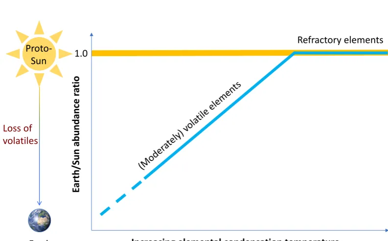
[image:25.595.122.519.179.426.2]

Refractory elements

Figure 1.1: Schematic illustration of the devolatilization of the solar nebula that formed the Earth: while refractory elements above a certain threshold condensation temperature could form rocky material, volatile material was lost, with increasing depletion corresponding to lower condensation temperature.

A characteristic feature of the comparison between solar and terrestrial abun-dances, is the depletion of terrestrial abundances for elements with moderately low condensation temperatures. This depletion is systematic: the lower the condensa-tion temperature, the greater the deplecondensa-tion, as illustrated schematically in Figure 1.1. This depletion provides quantitative insights into the processes active in the early solar system and the fractionation of elements between gas and solid phases.

This feature of volatile depletion has been previously investigated and is called the “volatility trend” of the Earth in the literature [Kargel and Lewis, 1993; Mc-Donough, 2003, 2014; Palme and O’Neill, 2003, 2014; Carlson et al., 2014]. An exam-ple is shown in Figure 1.2, which compares the elemental compositions between the bulk silicate Earth (i.e. the bulk Earth excluding the core) and CI chondrites, as a function of the elemental 50% condensation temperature,TC.

(26)

Figure 1.2: The volatility trend, illustrated by the wedge in gray, is shown as a com-parison of the elemental abundances of the bulk silicate Earth (i.e. the outer part of the Earth, essentially made by silicates) to CI chondritic abundances (normalized to 1) as a function of the 50% condensation temperature [Lodders, 2003]. The figure is from Palme and O’Neill [2014]. The normalization-reference element is Mg. The leg-end indicates the classification of elements according to their geochemical character: lithophile (elements) preferring to be in the silicate shell/mantle rocks, siderophile tending to be in the metal phase (i.e. core), chalcophile partitioning into sulfides. Above the legend, ‘HSE’ is the abbreviation of ‘highly siderophile elements’. ‘Main comp.’ near the upper x-axis denotes ‘Main components’, which are elements abun-dant in the Earth.

(27)

§1.1 From the Solar Nebula to the Planet Earth: Devolatilization Matters 9

models, or in the data.

In order to establish a chemical relationship between the proto-Sun and the bulk Earth to the highest precision possible, we need the best elemental abundance data (with uncertainties) to compare and quantify the differences between the two bodies.

1.1.3 Elemental abundances of the proto-Sun and the bulk Earth

For decades the combination of solar photospheric abundances and CI chondritic abundances have yielded what are thought to be the best proxy for the protosolar or solar system elemental abundances [e.g. Anders and Grevesse, 1989; Grevesse and Sauval, 1998; Lodders, 2003; Lodders et al., 2009]. As an example, Figure 1.3 shows the widely used compilation of protosolar abundance estimates of Lodders et al. [2009]. However, some information in their compilations needs to be readdressed and updated. First, CI chondritic abundances have been updated since 2009, e.g., by Barrat et al. [2012], Pourmand et al. [2012], and Palme et al. [2014]. Second, the solar photospheric abundances that they compiled are outdated and based on a het-erogeneous sample using different solar model atmospheres and radiative transfer calculations. In particular, their compilation does not use recent results based on 3D hydrodynamic solar models with radiative transfer calculations taking into account non-LTE (local thermodynamic equilibrium). Third, their approach of applying dif-fusion corrections to the combined solar abundances from both meteoritic and pho-tospheric data is questionable, since atomic diffusion and gravitational settling affect photospheric abundances, but not meteoritic abundances. Motivated by these issues, we redetermine the protosolar abundances from the recently updated meteoritic and photospheric data with an improved approach of combining the two data sets. This work is presented in Chapter 3.

For Earth, the estimates for its elemental abundances are not straightforward and are in large part model-dependent. A major challenge to estimating the bulk chemical composition of the Earth is that we can only sample the upper part of the possibly heterogeneous mantle, and we have no direct access to its deep interior, and even less to the core [Allègre et al., 2001]. But over the decades much progress has been made in making more plausible models of both the primitive mantle and the core, though usually separately. “Primitive mantle” or “bulk silicate Earth” are synonymous referring to the mantle after core segregation but before the extraction of continental crust. Thus, it is a reservoir equivalent to the combination of the present-day mantle and crust of the Earth. Studies of primitive mantle elemental abundances have been made based on a variety of models, e.g., Kargel and Lewis [1993], McDonough and Sun [1995], Lyubetskaya and Korenaga [2007], O’Neill and Palme [2008], and Palme and O’Neill [2014]. Studies of the elemental abundances of bulk Earth include Allègre et al. [2001], McDonough [2003], and McDonough and Arevalo [2008].

(28)

affini-Figure 1.3: Lodders et al. [2009]’s Solar System abundances (normalized to 106 _Si

atoms), which are a combination of the elemental abundances of CI chondrites and the solar photosphere.

ties of light elements for iron [Ricolleau et al., 2011; Mookherjee et al., 2011]. Seismic velocities through the core provide increasingly precise constraints on densities and on mineral physics models [Voˇcadlo, 2007; Li and Fei, 2014; Badro et al., 2014]. At the same time, better subduction models [Poitrasson and Zambardi, 2015] and estimates of the degree of homogeneity of the mantle [Javoy et al., 2010; Nakajima and Steven-son, 2015; McDonough, 2016] provide new constraints that are being included in the upper and lower mantle abundance estimates. Better observations of geo-neutrinos [Bellini et al., 2010; Gando et al., 2011; Bellini et al., 2013; Gando et al., 2013] also provide new thermal constraints for the abundances of heat-producing elements in the Earth [e.g. Sramek et al., 2013; Huang et al., 2013].

[image:28.595.85.469.96.326.2]

(29)

§1.2 From the Interstellar Medium to Our Planetary System 11

1 .

2 From the Interstellar Medium to Our Planetary System:

A Perspective of Chemical Inheritance

While planets form from stellar nebulae – i.e. the same material as the host star forms from – the origin of that material in turn is the interstellar medium (ISM). Interestingly, the interstellar medium exhibits a depletion of certain elements com-pared to the chemical composition of nearby young stars. This is surprising since these stars must have formed from the nearby interstellar medium, and exhibit very homogeneous abundances. The cause of the depletion must therefore be a process that occurs in the interstellar medium.

Investigations of UV spectra of stars since the 1970s have revealed interstellar absorption features produced by atoms in their favored ionization stages in the inter-stellar medium [Jenkins, 2009]. Atomic abundances of heavy elements relative to that of hydrogen are found to be below the reference cosmic abundances (approximated by solar abundances in our part of the Galaxy), to varying degrees. The reduction of heavy elements represents the missing atoms in the ISM gas phase. This feature is reinforced by the correlation of the abundance deficiencies of such elements with the temperatures derived theoretically for particle condensation in stellar nebulae, sug-gesting that these elements have condensed into dust grains [Field, 1974]. In a study of abundances along 243 different sight lines from more than 100 papers, Jenkins [2009] characterized the systematic patterns for depletions of 17 different elements (C, N, O, Mg, Si, P, S, Cl, Ti, Cr, Mn, Fe, Ni, Cu, Zn, Ge, and Kr), from which a unified quantitative scheme was constructed to estimate dust compositions.

(30)

otherwise these volatiles would have considerably evaporated. These carbonaceous chondrites are subdivided into the sub-classes/groups, e.g., CI, CM, CV, CO, CR, and CK [Weisberg et al., 2004], according to their chemical and mineralogy differences.

Figure 1.4: (a) Interstellar gas phase abundances relative to solar and (b) primitive meteoritic abundances relative to CI chondrites, as a function of the 50% condensa-tion temperature [Lodders, 2003]. For these moderately volatile elements, the gas of the interstellar medium and the meteorites show opposite abundance trends. The figures are from Yin [2005].

By comparing interstellar gas and dust composition with primitive meteoritic data, Yin [2005] demonstrated a remarkable qualitative similarity in the depletion patterns between the ISM and primitive meteorites for moderately volatile elements. This similarity is further discussed in Wang and Lineweaver [2016] and shown in Figure 1.4.

Note however that the depletion scales in the ISM gas phase and the meteoritic data differ by orders of magnitude, despite the qualitatively similar (but opposite) behavior. This can be explained if the depletion pattern found in the ISM gas phase is due to the condensation of the depleted elements onto interstellar dust grains. These dust grains with the condensed layer of volatiles are processed during the collapse stage of the parent molecular cloud and in the early active solar nebula through the processes such as shock-wave compression, vaporization and recondensation, and then form the so-called primitive meteorites through further fractionation, accretion, aerodynamic heating (when passing through the Earth’s atmosphere), and weather-ing (on the surface of the Earth). Despite this multitude of processes, it is strikweather-ing how well the overall abundance pattern of the interstellar dust grains is preserved in the primitive meteorites.

The important connection between the early solar nebula and the interstellar medium was outlined in a model by Yin [2005], which explains how interstellar grains act to seed the formation of primitive meteorites. The schematic in Figure 1.5 illustrates this connection, and can be explained as follows.

(31)

§1.2 From the Interstellar Medium to Our Planetary System 13

Diffuse ISM

(hot ionized gas and dust grains)

Molecular Clouds

(

molecular gas and dust

grains with condensed icy mantle)

Dust grain core

(possible growth of some grains)

Icy mantle

(e.g. H2O/CO/CO2Ices)

[image:31.595.77.540.104.342.2]

Protoplanetary Disk

(Stellar nebula with the central proto-Star)

Figure 1.5: Schematic processes of dust grains inherited from the interstellar medium into the protoplanetary disk. This figure is adapted from Wang and Lineweaver [2016].

the volatile elements (i.e. elements with low condensation temperatures) are in the hot ionized gas phase, while the refractory elements (i.e. elements with high con-densation temperatures) have condensed into dust grains.

(ii) In the cold and dense molecular cloud stage, the gas phase primarily con-sists of hydrogen molecules and helium. Carbon-rich species condense with other volatile elements onto the dust grain core. Accumulation of individual grains with icy mantles may occur at this stage, leading to the growth of dust grains.

(iii) As the gas pressure increases, the densest molecular cloud cores collapse, leading to the rapid formation of stellar nebulae. During the collapse of the cloud, the conservation of angular momentum leads to the formation of a protoplanetary disk. The disk rapidly flattens. The icy mantles (volatile compounds) on the surface of grains vaporize or sublimate if grains experience sudden heating, due to either adiabatic compression or shock waves.

(32)

1 .

3 Exoplanetary Chemistry and Interiors: A Growing

Path-way to Characterize Exoplanets and Habitability

With devolatilization likely to be an essential feature of terrestrial planet formation, the bulk elemental composition of terrestrial planets orbiting other stars can be esti-mated by devolatilizing the observed elemental abundances of those host stars. But why and how is the planetary bulk composition important for characterizing exo-planets and their habitability?

This question is pertinent to the prevalent modeling of exoplanetary interiors including structure and mineralogy [e.g. Dorn et al., 2017b; Brugger et al., 2017; Unterborn et al., 2018]. Exoplanetary interiors can influence mantle convection and surface recycling, i.e. planet tectonics, which in turn affects the outgassing of a planet and the formation of a secondary atmosphere [Noack and Breuer, 2014], thereby, the habitability of an extrasolar planet. To model exoplanetary interiors, we need two sets of principal observational constraints. One set is the planetary mass and radius information, and the other is the host stellar abundances. With only mass and radius measurements multiple solutions of interior composition and structure are possible, thus the problem is highly underconstrained or degenerate [Seager et al., 2007; Rogers and Seager, 2010]. My study on this topic therefore focuses on the other principal constraint – the elemental abundances of host stars, by taking into account devolatilization (see the schematic in Figure 1.6).

Recent studies [e.g. Dorn et al., 2015; Santos et al., 2015] have proposed adding host stellar abundances as a principal constraint to reduce the degree of modeling degeneracy of exoplanetary interior structure and mineralogy. However, one fact that is ignored consistently in the prevalent exoplanetary interior models [e.g. Dorn et al., 2015; Santos et al., 2015; Dorn et al., 2017b; Brugger et al., 2017; Unterborn et al., 2018] is that the elemental abundances of a rocky exoplanet arenotidentical to the elemental abundances of its host star. Host stellar abundances are good proxies of planetary abundances, but only for refractory elements (i.e. elements with con-densation temperatures& 1360 K). This is particularly true for terrestrial planets, as evidenced by the relative compositional differences between the Sun, Earth and other inner solar system bodies [Davis, 2006; Carlson et al., 2014].

(33)

§1.3 Exoplanetary Chemistry and Interiors 15

Planetary

mass

Planetary

radius

Exoplanetary

chemistry

and interiors

Host stellar

abundances

Radial velocity

Transit photometry

Spectroscopic measurements

Devolatilize

Planetary bulk

composition

Figure 1.6: Observational information required for modeling exoplanetary chemistry and interiors. It is recommended that host stellar abundances are devolatilized first to represent the planetary bulk composition, which is then used as a principal constraint for the modeling.

devolatilization pattern applies to other planetary systems.

Composition-, location-, and timescale-dependent differences in the various frac-tionation processes in a stellar nebula may lead to a variety of outcomes in the com-position of a rocky planet (see Figure 1.7). The comcom-positional differences between the Earth, Mars and Venus could be a measure of these variations within our own Solar System, but the extent to which the bulk compositions of Venus and Mars are different to the Earth is still debated [Morgan and Anders, 1980; Wanke and Dreibus, 1988; Taylor, 2013; Kaib and Cowan, 2015]. We also note that thebulk compositions of Venus and Mars are not well determined yet and thus reliable quantitative anal-ysis of bulk compositional differences between them and the Earth is difficult. In spite of the complexity of planet formation, an essential step to improve the study of exoplanetary chemistry is to take into account devolatilization, starting with the best constrainable trend coming from the Sun-to-Earth comparison.

(34)

400 600 800 1000 1200 1400 1600 1800 10-3

10-2 10-1 100

400 600 800 1000 1200 1400 1600 1800

50% Condensation Temperature (K) 10-3

10-2 10-1 100

Elemental Abundance Normalized to Al and the proto-Sun

Tl

I In

Br Cd

S Se Sn

Te Zn Pb

F

Bi Cs

Rb

Ge B

Cl Na

Ga

Sb Ag

KCu Au As

Li

Mn P

Cr

Si

Pd Fe

Mg CoNi

Eu

RhPt Ca

Ti Al

CI (Palme+2014)

CM (Wasson & Kallemeyn 1988) Earth (Wang et al. 2018) Mars (Taylor 2013)

[image:34.595.76.481.114.398.2]

Venus (Morgan & Anders 1980)

Figure 1.7: The elemental composition of solar system rocky bodies, including CI chondrites [Palme et al., 2014], CM chondrites [Wasson and Kallemeyn, 1988], Earth [Wang et al., 2018a], Mars [Taylor, 2013], and Venus [Morgan and Anders, 1980], normalized to the protosolar elemental abundances [Wang et al., 2018b], on the equal basis of 106 _{Al atoms. In Taylor [2013], the elemental composition of Mars is the}

primitive Martian mantle composition, so only lithophile elemental abundances are plotted here. The abundance differences between terrestrial planets are not clearly distinguishable.

(35)

§1.4 Thesis Outline 17

noting that sulfur abundance in a rocky exoplanet should result from devolatilizing the host star, prior to the further fractionation of sulfur within the planet body.

1 .

4 Thesis Outline

This thesis presents new estimates for the elemental abundances of the bulk Earth and proto-Sun. The differences quantify the devolatilization processes pertaining to the formation of the rocky planets of our Solar System. This quantification is, by extension, applicable to other planetary systems to infer the exoplanetary bulk compositions from their known host stellar abundances. We also explore constraints that can be improved to advance studies of exoplanetary interior and habitability.

Chapter 2 presents our concordance estimates for the elemental abundances with uncertainties of the primitive mantle, the core, and the bulk Earth. This work allows the comparison between the Earth and the Sun, as well as other solar system bodies, to study the accretion and fractionation processes that produce rocky planets from protoplanetary nebulae.

Chapter 3 extends our analysis of terrestrial abundances to the estimates of pro-tosolar elemental abundances based on the latest estimates of solar photospheric abundances and primitive meteoritic abundances, and then to establish a fiducial model from the Earth-to-Sun abundance ratios as a function of elemental condensa-tion temperatures. This model provides quantitative insights into the devolatilizacondensa-tion processes associated with the formation of rocky planetary bodies.

Chapter 4 applies the fiducial devolatilization model to nearby planetary sys-tems to infer the bulk elemental composition of rocky exoplanets – particularly those within the circumstellar habitable zones – from the known host stellar abundances. The estimated planetary bulk composition (rather than the host stellar abundances) is then used as a principal constraint (along with other assumptions) to model the interior composition and structure of such exoplanets, which are essential to under-standing their habitability.

(36)

(37)

Chapter2

The Elemental Abundances (with

Uncertainties) of the Most

Earth-like Planet

This chapter is adapted from Wang et al. [2018a] originally published as

Wang, H. S., Lineweaver, C. H., and Ireland, T. R. 2018. The Elemental Abun-dances (with Uncertainties) of the Most Earth-like Planet. Icarus 299, 460-474,doi. org/10.1016/j.icarus.2017.08.024

Abstract

To first order, the Earth as well as other rocky planets in the Solar System and rocky exoplanets orbiting other stars, are refractory pieces of the stellar nebula out of which they formed. To estimate the chemical composition of rocky exoplanets based on their stellar hosts’ elemental abundances, we need a better understanding of the devolatilization that produced the Earth. To quantify the chemical relationships be-tween the Earth, the Sun and other bodies in the Solar System, the elemental abun-dances of the bulk Earth are required. The key to comparing Earth’s composition with those of other objects is to have a determination of the bulk composition with an appropriate estimate of uncertainties. Here we present concordance estimates

(with uncertainties) of the elemental abundances of the bulk Earth, which can be used

in such studies. First we compile, combine and renormalize a large set of hetero-geneous literature values of the primitive mantle (PM) and of the core. We then integrate standard radial density profiles of the Earth and renormalize them to the current best estimate for the mass of the Earth. Using estimates of the uncertainties in i) the density profiles, ii) the core-mantle boundary and iii) the inner core boundary, we employ standard error propagation to obtain a core mass fraction of 32.5_±0.3 wt%. Our bulk Earth abundances are the weighted sum of our concordance core abundances and concordance PM abundances. Unlike previous efforts, the

(38)

(39)

§2.1 Introduction 21

2 .

1 Introduction

The number of known rocky exoplanets is rapidly increasing. Transit photometry and radial velocity measurements, when combined, yield rough estimates of the densities and therefore mineralogies of these exoplanets. Independent and poten-tially more precise estimates of the chemical composition of these rocky planets can be made based on the known elemental abundances of their host stars combined with estimates of the devolatilization process that produced the rocky planets from their stellar nebulae. To proceed with this strategy, we need to quantify the de-volatilization that produced the Earth from the solar nebula. Knowledge of the bulk elemental abundances of the Earth with uncertainties is an important part of this research. The elemental abundances of bulk Earth (including both the bulk silicate Earth and the core) can tell us a more complete story of the potentially universal accretion and fractionation processes that produce rocky planets from nebular gas during star formation. Uncertainties associated with the bulk Earth composition are needed to compare and quantify compositional differences between the Earth, Sun, and other solar system bodies. Such comparisons can lead to a more detailed un-derstanding of devolatilization and the chemical relationship between a terrestrial planet and its host star. The bulk Earth elemental abundances will help determine what mixture of meteorites, comets and other material produced the Earth [Drake and Righter, 2002; Burbine and O’Brien, 2004] and can also help determine the width of the feeding zone of the Earth in the protoplanetary disk [Chambers, 2001; Kaib and Cowan, 2015].

There are many stages of compositional fractionation between the collapse of a stellar nebula, the evolution of a protoplanetary disk and a final rocky planet. Composition- and position-dependent differences in the duration and strength of the various fractionating processes can lead to a variety of outcomes. The different (but somewhat similar) compositions of Earth, Mars and Vesta are a measure of these variations within our own Solar System.

A major challenge to estimating the bulk chemical composition of the Earth is that we can only sample the upper part of the possibly heterogeneous mantle, and we have no direct access to its deep interior, and even less to the core [Allègre et al., 2001]. Early studies on primitive mantle (PM) elemental abundances include O’Neill [1991], Kargel and Lewis [1993], McDonough and Sun [1995], and O’Neill and Palme [1998]. Bulk elemental abundances with uncertainties [Allègre et al., 2001] were re-ported 16 years ago but much work on PM abundances and on core abundances (usually separately) has been done since then [e.g., Lyubetskaya and Korenaga, 2007; Palme and O’Neill, 2014; Rubie et al., 2011; Wood et al., 2013; Hirose et al., 2013]. The determination of uncertainties is central to the quantification of elemental abun-dances but has been a missing priority in previous work. The most recent, highly cited estimates of the elemental abundances of the bulk Earth do not include uncer-tainties [McDonough, 2003; McDonough and Arevalo, 2008].

(40)

plau-sible models. Our knowledge of the core (and therefore of the bulk Earth) has in-creased significantly: high pressure experiments yield improved partition coefficients of siderophiles [Siebert et al., 2013] and improved affinities of light elements for iron [Ricolleau et al., 2011; Mookherjee et al., 2011]. Seismic velocities through the core provide increasingly precise constraints on densities and on mineral physics mod-els [Voˇcadlo, 2007; Li and Fei, 2014; Badro et al., 2014]. Better subduction modmod-els [Poitrasson and Zambardi, 2015] and estimates of the degree of homogeneity of the mantle [Javoy et al., 2010; Nakajima and Stevenson, 2015; McDonough, 2016] provide new constraints that are being included in the upper and lower mantle abundance estimates. Better observations of geo-neutrinos [Bellini et al., 2010; Gando et al., 2011; Bellini et al., 2013; Gando et al., 2013] provide new thermal constraints for the abundances of heat-producing elements in the Earth [e.g. Sramek et al., 2013; Huang et al., 2013]. The large majority of the literature on elemental abundances of the Earth, involving either the analysis of the PM or of the core, are increasingly impor-tant and when combined, yield improved elemental abundances of the bulk Earth composition and more realistic uncertainties.

Our main research goal is to analyze the compositional differences between the Earth, Sun and other solar system bodies and from this comparison quantify the de-volatilization of stellar material that leads to rocky planets. This requires estimates of the bulk Earth abundanceswith uncertainties. These bulk abundances and their uncer-tainties are poorly constrained and often ignored in the literature. Motivated by this, we make a concordance estimate of the bulk Earth elemental abundances and their uncertainties. The words “concordance estimate” specifically mean a compositional estimate that is representative of, and concordant with previous estimates. The aim of this work therefore is not to resolve the discrepancies between competing mod-els and assumptions but to construct a concordance model (with uncertainties) that represents current knowledge of bulk Earth composition and calibrates unresolved discrepancies. We envisage that if the discrepancies can be resolved, a better formula-tion for estimating uncertainties might be forthcoming. However, at this stage, some of the arguments concerning the derivation of models, or values resulting from these models, appear intractable. Nevertheless, there is an essential need for uncertainties in the estimates if we are to make progress in comparing planetary objects.

2 .

2 Composition of the Primitive Mantle

2.2.1 Data sources

Earth’s primitive mantle (PM) or bulk silicate Earth (BSE) is the mantle existing af-ter core segregation but before the extraction of continental and oceanic crust and the degassing of volatiles [Sun, 1982; Kargel and Lewis, 1993; Saal et al., 2002; Mc-Donough, 2003; Lyubetskaya and Korenaga, 2007; Palme and O’Neill, 2014]. There are two major, and partially-overlapping modeling strategies for estimating the PM composition.

(41)

§2.2 Composition of the Primitive Mantle 23

periodotite massifs. Peridotite-basalt melting trends yield an estimate of the PM com-position [e.g., Ringwood, 1979; Sun, 1982; McDonough and Sun, 1995; McDonough, 2003; Lyubetskaya and Korenaga, 2007]. The peridotite model has a number of in-trinsic problems, including the non-uniqueness of melting trends, large scatter in the data from mid-ocean ridge basalts (MORB) and from ocean island basalts (OIB), and the difficulty of imposing multiple cosmochemical constraints on refractory lithophile element (RLE) abundances, often resulting in model-dependent, poorly quantified uncertainties [Lyubetskaya and Korenaga, 2007].

The cosmochemical model is based on the identification of Earth with a particu-lar class of chondritic or achondritic meteorites or their mixtures [e.g., Morgan and Anders, 1980; Javoy et al., 2010; Fitoussi et al., 2016], along with a number of as-sumptions on accretion and fractionation processes [Allègre et al., 2001]. The cosmo-chemical model uses chondritic ratios of RLEs and volatility trends [e.g., Wanke and Dreibus, 1988; Palme and O’Neill, 2003, 2014]. Palme and O’Neill [2003] and Palme and O’Neill [2014] present a core-mantle mass balance approach for calculating the primitive mantle composition. This approach requires an accurate determination of magnesium number (Mg # = molar Mg/(Mg+Fe)). A reasonable range for Mg# can be inferred from fertile mantle periodites.

Our aim is not to resolve the differences between these strategies and models but to construct a concordance model whose mean values and uncertainties adequately represent current knowledge and disagreement.

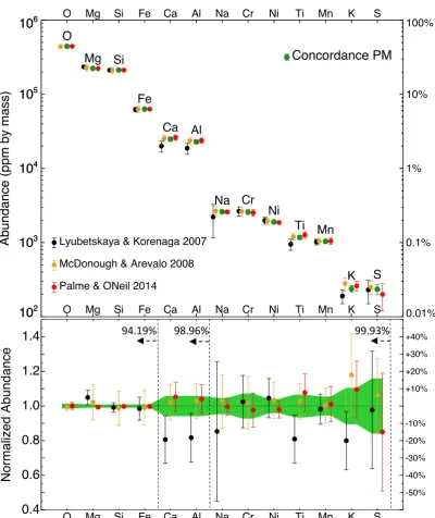
2.2.2 Concordance PM estimate

We construct our concordance PM abundances from three major papers reporting PM abundances [Lyubetskaya and Korenaga, 2007; McDonough and Arevalo, 2008; Palme and O’Neill, 2014], supplemented with noble gas abundances from Marty [2012] and Halliday [2013]. McDonough and Arevalo [2008] is an updated version of their pioneering peridotite model [McDonough and Sun, 1995; McDonough, 2003]. Updates of some abundances, for example W, K and Pb, can be found in Arevalo and McDonough [2008] and Arevalo et al. [2009]. Lyubetskaya and Korenaga [2007] performed a principal component analysis of the same peridodite database but with different model parameters. Palme and O’Neill [2014] is largely based on a cosmo-chemical model using mass balance and is an updated version of their pioneering earlier work [Palme and O’Neill, 2003].

Challenges to combining these three data sets are:

i) McDonough and Arevalo [2008] report no uncertainties, however the PM abun-dance uncertainties reported in McDonough and Sun [1995] approximately reflect current uncertainties. Thus, in our analysis, we attach them to the PM abundances reported in McDonough and Arevalo [2008].

ii) Lyubetskaya and Korenaga [2007] do not report abundances of four volatiles; C, H, N, O.

(42)

10-7 10-6 10-5 10-4 10-3 10-2 10-1 100 101 102 103 104 105 106 10-7 10-6 10-5 10-4 10-3 10-2 10-1 100 101 102 103 104 105 106

Abundance (ppm by mass)

10-6 10-5 10-4 10-3 10-2 10-1 100 101 102 103 104 105 106

O Mg Si Fe Ca Al Na Cr Ni Ti Mn K S C H Co V P Zn Cu Sr F Cl Sc Zr Ba Ga Y N Ce Li Nd Ge Dy La Nb Gd Rb Yb Er Sm Hf Pr B Pb Eu Ho Sn Tb Se Th Tm Lu Be As Br Mo Ta Cd U Cs In W Te I Pt Hg Pd Ru Sb Ag He Os Ir Bi Tl Rh Au Re Ar Ne Kr Xe

O Si Ca Na Ni Mn S H V Zn Sr Cl Zr Ga N Li Ge La Gd Yb Sm Pr Pb Ho Tb Th Lu As Mo Cd Cs W I Hg Ru Ag Os Bi Rh Re Ne Xe

Lyubetskaya & Korenaga 2007

McDonough & Arevalo 2008

Palme & ONeil 2014

Halliday 2013 (layered mantle) Halliday 2013 (impact erosion) Halliday 2013 (basaltic glass) Marty 2012 (atmospheric)

Concordance PM O Si Ca Na Ni Mn S H V Zn SrCl Zr Ga N Li Ge

La Gd Yb Sm Pr

Pb Ho

Tb Th_{Lu As Mo Cd}

Cs W I Hg

Ru Ag Os Bi Rh Re Mg Fe Al Cr Ti K C Co P

Cu F Sc Ba

Y Ce

Nd Dy

Nb Rb Er Hf

B Eu Sn

Se Tm Be Br Ta U In Te Pt Pd Sb _Ir Tl Au He Ar Ne Kr Xe 0.0 0.5 1.0 1.5 2.0 2.5 3.0 Normalized Abundance 0.0 0.5 1.0 1.5 2.0 2.5 3.0 Mg Fe Al Cr Ti K C Co P Cu F Sc Ba Y Ce Nd Dy Nb Rb Er Hf B Eu Sn Se Tm Be Br Ta U In Te Pt Pd Sb He Ir Tl Au Ar Kr

O Si Ca Na Ni Mn S H V Zn Sr Cl Zr Ga N Li Ge La Gd Yb Sm Pr Pb Ho Tb Th Lu As Mo Cd Cs W I Hg Ru Ag Os Bi Rh Re Ne Xe Br

Mg Fe Al Cr Ti K C Co P Cu F Sc Ba Y Ce Nd Dy Nb Rb Er Hf B Eu Sn Se Tm Be Ta U In Te Pt Pd Sb He Ir Tl Au Ar Kr

Decreasing PM Abundance -->

[image:42.595.72.485.90.594.2]

3.5 3.5 3.6 6.0 3.6 3.6 6.0 3.6 3.6 6.0 3.6 4.3

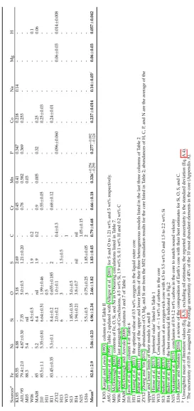
Figure 2.1: Recent literature estimates of 83 elemental abundances in the primitive mantle (PM) and our concordance estimates (green) constructed from them. Ele-ments are plotted in order of decreasing PM abundance. The upper panel plots ppm by mass. In the lower panel, literature values have been normalized to our PM con-cordance estimates. Our PM concon-cordance ppm estimates have been rescaled up by 0.3% to ensure that their sum equals 106_{. We have not rescaled the literature values}

(43)

§2.2 Composition of the Primitive Mantle 25

102 103 104 105 106

Abundance (ppm by mass)

0.01% 0.1% 1% 10% 100%

O Mg Si Fe Ca Al Na Cr Ni Ti Mn K S

O

Mg Si

Fe

Ca _Al

Na Cr Ni

Ti _Mn

K S

Lyubetskaya & Korenaga 2007

McDonough & Arevalo 2008

Palme & ONeil 2014

Concordance PM

-50% -40% -30% -20% -10% +10% +20% +30% +40%

0.4 0.6 0.8 1.0 1.2 1.4

Normalized Abundance

O Mg Si Fe Ca Al Na Cr Ni Ti Mn K S

[image:43.595.119.520.118.595.2]

94.19% 98.96% 99.93%

(44)

In, Hg, Bi, Ag, Cd and Tl. We assign the McDonough and Sun [1995] uncertainties to these elements.

iv) none of these three PM models include noble gas abundances. In a prelim-inary attempt to be more comprehensive, we supplement these three PM models with recent noble gas abundances: the atmospheric model of Marty [2012] and three different models (layered mantle, impact erosion, and basaltic glass) from Halliday [2013]. This range encompasses recent results from Dauphas and Morbidelli [2014] [Marty et al., 2016]. See Appendix A.1 for details.

The resultant concordance estimates for the PM elemental abundances and their uncertainties are listed in column 3 of Table 2.1. Our PM elemental abundances are increased by 0.3% to ensure that the sum of all the ppm values equals 106 _(see

A.3). Figs. 2.1 & 2.2 show the comparison of our concordance abundances with the literature values. The upper panel of Fig. 2.1 shows elemental abundances (ppm by mass). The literature abundances normalized to our concordance PM abundances are shown in the lower panel. For clarity, Fig. 2.2 is a zoomed-in version of the 13 most abundant elements in Fig. 2.1. The abundances of these 13 elements account for 99.93+0.07_0.72 wt% of the primitive mantle.

By construction, our concordance PM abundances are consistent with the litera-ture abundances. There are some outliers. For example, the Lyubetskaya and Kore-naga [2007] abundances of Cl and Br are relatively low because they used the Cl/K ratio of 0.0075±0.0025 from highly depleted MORB in Saal et al. [2002]. This ratio is

⇠ 10 times lower than an equivalent Cl/K ratio of⇠ 0.07 used in McDonough and Arevalo [2008] [which came from the Cl/Rb⇠ 28 and K/Rb ⇠ 400 of McDonough and Sun, 1995]. The abundances of K estimated in Lyubetskaya and Korenaga [2007] and McDonough and Arevalo [2008] are consistent (190±76 ppm and 240±48 ppm, respectively), resulting in the abundance of Cl in Lyubetskaya and Korenaga [2007]⇠

(45)

(46)

[image:46.595.73.424.174.670.2]

(47)

§2.3 Composition of the Core 29

2 .

3 Composition of the Core

2.3.1 Data sources

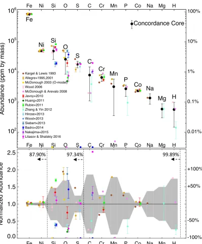
The density deficit of the Earth’s core (compared to a pure Fe-Ni composition) sug-gests that the core contains a significant amount of one or more light elements. The liquid outer core is thought to have a density deficit of 3 12 wt% [e.g., Stevenson, 1981; Anderson and Ahrens, 1994; McDonough, 2003], while the solid inner core is 3-6 wt% less dense than predicted [e.g., Anderson and Ahrens, 1994; Hemley and Mao, 2001]. The candidate light elements are still controversial and have been mod-eled and estimated in various ways and plausibly include Si, O, S and C [e.g. Fitoussi and Bourdon, 2012; Hirose et al., 2013; Litasov and Shatskiy, 2016].

We have compiled and combined a wide variety of recent work to construct concor-dance core abunconcor-dances. These are listed in Tables 2.1 and 2.2 and include various constraints from various core compositional models, terrestrial fractionation curves and mass balance [e.g. Kargel and Lewis, 1993; Allègre et al., 1995; McDonough, 2003; Wood et al., 2006; McDonough and Arevalo, 2008], metal-silicate equilibrium [e.g. Rubie et al., 2011], the chemistry of core formation [e.g. Javoy et al., 2010], high-pressure and high-temperature experiments [Siebert et al., 2013], experiments based on sound velocity and/or density jumps [Huang et al., 2011; Nakajima et al., 2015], and numerical simulations [e.g. Zhang and Yin, 2012; Badro et al., 2014].

2.3.2 Concordance core estimate

Since many core abundances reported in the literature are model-dependent and are given without uncertainties, our concordance abundances (Tables 2.1 and 2.2) are unweighted averages (Eq. A.3) and exclude abundances that have been set to zero. Based on mass balance between the core and the silicate Earth, McDonough [2003] proposed both Si-bearing and O-bearing core models while McDonough and Arevalo [2008] presented a Si-bearing model only. The trace elements in the Mc-Donough [2003] O-bearing model and McMc-Donough and Arevalo [2008] Si-bearing model are highly correlated. Therefore we only count them once in our calculations. The details of how the literature values were combined into our concordance values with uncertainties are described in A.1.2.

Fig. 2.3 shows our concordance abundances for 49 elements in the core, compared with the literature values from which they were constructed. The sum of our concor-dance abunconcor-dances of the 49 elements is scaled to 106 _{and listed in column 5 of Table}

(48)

[image:48.595.152.426.163.743.2]

Devolatilization During the Formation of Rocky Planets: Bulk Elemental Composition