Effect of the Pauli Exclusion Principle in the Many-Electron Wigner Function

arXiv:cond-mat/0703185v1 [cond-mat.other] 7 Mar 2007

The Effect of the Pauli Exclusion Principle in the Many-Electron Wigner Function

Emiliano Cancellieri, Paolo Bordone and Carlo Jacoboni

Dipartimento di Fisica Universit`a di Modena e Reggio Emilia and CNR-INFM S3 National Research Center, via Campi 213/a, 41100 Modena (Italy).

(Dated: February 6, 2008)

An analysis of the Wigner function for identical particles is presented. Four situations have been considered. i) A scattering process between two indistinguishable electrons described by a minimum uncertainty wave packets showing the exchange and correlation hole in Wigner phase space. ii) An equilibrium ensemble of N electrons in a one-dimensional box and in a one-dimensional harmonic potential showing that the reduced single particle Wigner function as a function of the energy defined in the Wigner phase-space tends to a Fermi distribution. iii) The reduced one-particle transport-equation for the Wigner function in the case of interacting electrons showing the need for the two-particle reduced Wigner function within the BBGKY hierarchy scheme. iv) The electron-phonon interaction in the two-particle case showing co-participation of two electrons in the interaction with the phonon bath.

PACS numbers: 05.30.Fk; 63.20.-e; 72.10.-d

I. INTRODUCTION

Highly sophisticated technologies produce physical sys-tems, and in particular semiconductor devices, of very small dimensions, comparable with electron wavelength or with electron coherence lengths. Under such condi-tions, semi-classical dynamics is not justified in principle and interference effects due to the linear superpositions of quantum states have to be considered. Among the possible different approaches, the Wigner-function (WF) has proved to be very useful for studying quantum elec-tron transport [1, 2, 3, 4], owing to its selec-trong analogy with the semiclassical picture, since it explicitly refers to variables defined in an (r,p) Wigner phase space, to-gether with a rigorous description of electron dynamics in quantum terms.

In this work we present an analysis of the WF for iden-tical particles. Even thought the WF was defined from its very beginning for the study of many-particle physics, in electron transport theory it has been used mainly in its one-particle version. The importance of the many-body problem derives from the fact that any real physical sys-tem one can think of is composed of a set of interacting bodies. Moreover, since we are dealing with quantum me-chanical systems the symmetry properties that describe the behavior of identical particles play an essential role. The present paper will be focused mainly on the last sub-ject.

In particular, four situations will be analyzed: i) A scattering process between two indistinguishable elec-trons described by minimum uncertainty wave packets, showing the exchange and correlation hole in Wigner phase space. ii) An equilibrium ensemble of N electrons in a box and in a harmonic potential, showing that the sum of the values of the WF that correspond to points in the Wigner phase-space with energy in a given inter-val, tends to a Fermi distribution. iii) The transport

equation for interacting electrons, showing the BBGKY hierarchy when the integral, over the degrees of freedom of all the particles but one, are performed [5, 6]. iv) The electron-phonon interaction in the case of two particles, where new Keldysh diagrams [7] appear with respect to the one-electron case [8].

II. WIGNER FUNCTION FOR MANY IDENTICAL PARTICLES

The WF was introduced by Wigner in 1932 to study quantum corrections to classical statistical mechanics [1, 9, 10, 11]. Thus, even though it is now used mainly in single particle problems, from the very beginning this function was defined for N particles as:

fW(r1,p1, ...,rN,pN, t) =

Z

ds1...dsNe− i

~

P

sipi

×ψr1+

s1

2, ...,rN + sN

2 , t

×ψ⋆_r

1− s1

2, ...,rN− sN

2 , t

.

(1)

In the case of identical particles, the wave function de-scribing the many-body system satisfy well known sym-metry relations. When the position coordinates of two particles are interchanged the wave function remains un-affected (bosons) or changes sign (fermions). Since the WF is bilinear in the wave function it remains the same if the positions and, accordingly, the Wigner momenta of two particles are exchanged.

fW(N)(r1,p1, ...,rM,pM, t) =

N!

(N−M)!h3(N−M) Z

drM+1dpM+1...drNdpNfW(r1,p1, ...,rN,pN, t), (2)

where the superscript (N) indicates that the reducedM -particle WF is defined in a system withNparticles. Note that in the case where M = 1 the above equation be-comes:

fW(N)(r1,p1, t) = N h3(N−1)

Z

dr2dp2...drNdpN

×fW(r1,p1, ...,rN,pN, t).

(3)

The factorials appearing in front of the integral in equa-tion (2) simplify to N in equation (3) since this is the number of equivalent ways one can reduce theN-particle WF when the particles themself are supposed to be iden-tical.

A. The WF for Many Single-Particle Wave Functions

We consider the case ofN particles in the system and we define the WF with a wave function that is a symmet-ric or anti-symmetsymmet-ric linear combination of single-particle wave functionsψi(r), (i= 1, ..., N) as

ψ(r1, ...,rN) = ψ1(r1)ψ2(r2)ψ3(r3)... ψN(rN)

±ψ1(r2)ψ2(r1)ψ3(r3)... ψN(rN)

+ψ1(r2)ψ2(r3)ψ3(r1)... ψN(rN)

±ψ1(r3)ψ2(r2)ψ3(r1)... ψN(rN)

+... (4)

where the upper sign is for bosons and the lower for fermions. In the WF expression it is possible to identify two different types of terms. The first one is character-ized by the product of single-particle WFs. In each of these contributions, from the different wave functions, N WF are obtained that are evaluated in a particu-lar permutation of the variable indices as, for example: fW1(r4,p4)fW2(r1,p1)fW3(r2,p2)...fWN(rN−5,pN−5).

The second type of contributions accounts for the ex-change effects and vanishes when the wave functions ψn(r) do not overlap. These terms are constituted by

in-tegrals of the product ofN factorsψnψn⋆, one for each of

theNwavefunctionsψn. In these terms at list two

prod-uctsψn(ri+si/2)ψn⋆(rj−sj/2) are evaluated withi6=j.

It is the presence of such factors that makes impossible to obtain the many-particle WF in terms of single-particle WFs. The number of factorsψnψn⋆, where ψn and ψn⋆

correspond to different particles, appearing in a given in-tegral can range from 2 toN. As an example the WF in the case ofN = 2 reads:

fW(r1,p1,r2,p2,) = fW1(r1,p1)fW2(r2,p2) +fW1(r2,p2)fW2(r1,p1)

±_~1₆

Z

ds1ds2e−

i

~(s1p1+s2p2)

×hψ1

r1+

s1 2

ψ⋆

1

r2− s2

2

ψ2

r2+ s2

2

ψ⋆

2

r1− s1

2

+ψ1

r2+ s2

2

ψ1⋆

r1− s1

2

ψ2

r1+ s1

2

ψ⋆2

r2− s2

2 i

,

(5)

here 4 terms appear, 2 for each kind of contribution. The two-particle system is treated in details in [14].

B. Example of Two Colliding Electrons

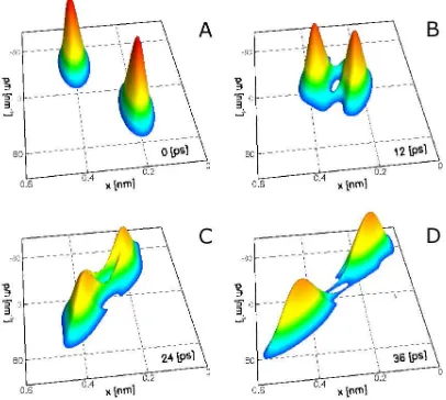
FIG. 1: One dimensional reduced single-particle WF of two interacting electrons at different times. The figure clearly shows the exchange hole due to the Pauli exclusion principle.

equation was solved with initial conditions given by two minimum-uncertainty wave packets interacting through the Coulomb potential and the WF was evaluated at dif-ferent time steps (see Fig. 1).

In this figure we plot the one-particle reduced WF of the system for the case of two Gaussian wave packets with opposite central wave vectors. Since we are dealing with a one dimensional system, the two particles are expected to

decelerate, scatter, and then move away from each other. Att = 0 we suppose the two particles to be described by an antisymmetric wave function. In Fig. 1.B the system is shown 2 ps after the Coulomb interaction is switched on. At the beginning of the scattering process the exchange hole due to the Pauli’s exclusion principle appears. In part 1.C the two particles are shown when their mutual distance has reached the minimum value. In this case the exchange hole is maximally evident. When the two particles are moving far enough from each other the exchange hole tends to disappear (part 1.D).

III. EQUILIBRIUM WF FOR NON INTERACTING PARTICLES IN CONFINED

POTENTIALS

In this section a system of N fermions in a confined potential has been studied. In the non-interacting case the one-particle reduced WF is studied at thermal equi-librium at a temperature ofT = 2 K. In order to simplfy the mathematical treatment we shall introduce the sec-ond quantization notation. TheN-particles wave func-tion can thus be written as:

ψ(r1, ...,rN) =hr1, ...,rN|ψi=h0|Ψ(ˆ r1)...Ψ(ˆ rN)|ψi,

(6) and the WF as:

fW(N)(r1,p1) =

N h3(N−1)

Z

dr2dp2...drNdpN

Z

ds1...dsNe− i

~

PN

j=1pjsj _×

D 0

Ψˆ

r1+ s1

2

...ΨˆrN +

sN

2 ψ

ED ψ

Ψˆ

†_r N −

sN

2

...Ψˆ†r1− s1

2 0

E ,

(7)

where, here and in the following, ˆΨ and ˆΨ† _{are the}

cre-ation and annihilcre-ation field operators. Since we are inter-ested in the thermal equilibrium distribution of a fixed number of particles, the density matrix in the above equa-tion is:

|ψihψ|= ˆρ= 1

Ze

− Hˆ

kB T_{, (8)}

where Z is the partition function, ˆH the Hamiltonian, kBthe Boltzman constant, andT the temperature of the

system. Since the particles in the system are supposed to be non interacting, and the system is supposed to be

confined, the Hamiltonian in its second quantization form can easely be written in terms of the particles creation ˆ

c†

n and annihilation operators ˆcn as:

ˆ

H =

∞

X

n=1

ǫnˆc†nˆcn, (9)

h0|...|0i = X n′ 1 ...X n′ N X n′′ 1 ...X n′′ N D 0

ˆcn′1...ˆcn′Ne − 1

kB T

P

nǫncˆ

†

nˆcn_ˆc† n′′

N...ˆc † n′′ 1 0 E ×

ψn′

1

r1+

s1 2

...ψn′

N

rN +

sN 2 ψ⋆ n′′ N rN−

sN 2 ...ψ⋆ n′′ 1 r1−

s1 2 = X n′ 1 ...X n′ N X n′′ 1 ...X n′′ N D 0

ˆcn′1...ˆcn′Ncˆ † n′′

N...ˆc † n′′ 1 0 E e− 1

kB T(ǫn′′

1+...+ǫn′′N)×

ψn′

1

r1+

s1 2

...ψn′

N

rN +

sN 2 ψ⋆ n′′ N rN−

sN 2 ...ψ⋆ n′′ 1 r1−

s1 2

, (10)

where ψn indicates the n-th eigenstate of the confining

potential. In order to better understand how to treat the above equation let us focus on the two-particle case. Using the fermionic or the bosonic commutation rules for the contribution containing the creation and annihilation operators, the following identity is achieved:

D 0

ˆcn′1ˆcn′2ˆc

† n′′

2cˆ

† n′′ 1 0 E = δn′

1n′′1δn′2n′′2 ±δn′1n′′2δn′2n′′1

. (11)

By substituting equation (11) into equation (10) for N= 2, and using it in equation (7) the following expres-sion is obtained:

fW(2)(r1,p1) = 2 h3_Z

Z

dr2dp2 Z

ds1ds2e−

i

~(s1p1+s2p2)X

n′

1

X

n′

2

e−kB T1 (ǫn′₁+ǫn′₂)

×nψn′

2

r2+

s2 2

ψn′

1

r1+

s1 2 ψ⋆ n′ 1 r1−

s1 2 ψ⋆ n′ 2 r2−

s2 2

±ψn′

1

r2+

s2 2

ψn′

2

r1+

s1 2 ψ⋆ n′ 1 r1−

s1 2 ψ⋆ n′ 2 r2−

s2 2

o

, (12)

then, performing the integrals, we finally get:

f_W(2)(r1,p1) = 2 Z X n′ 1 X n′ 2

e−kB T1 (ǫn′

1+ǫn′2)f_W

n′₁(r1,p1)

±2 Z X n′ 1 X n′ 2

e−kB T1 (ǫn′₁+ǫn′₂)_δ n′

2n′1

Z ds1e−

i

~s1p1_ψ

n′

2

r1+

s1 2 ψ⋆ n′ 1 r1−

s1 2 = 2 Z X n′ 1    X n′ 2

e−kB T1 (ǫn′

1+ǫn′2)±e− 1

kB T2ǫn′

1

 

 fW_n′

1(

r1,p1), (13)

where fWn1(r1,p1) indicates the WF of the n

th

1 eigen-state of the confined potential.

This expression can be written in a more compact form by identifying the bosonic and the fermionic cases:

f_Wbosons(2) (r1,p1) = 2 Z X n1 X n2 e−

ǫn1+ǫn2

kB T _fW

n1(r1,p1),

(14)

fW(2)f ermions(r1,p1) =

2

Z

X

n1

X

n26=n1

e−

ǫn1+ǫn2

kB T _fW

n1(r1,p1).

(15)

fW(Nbosons) (r1,p1) =

N

Z

X

n1,n2,...,nN

e−

ǫn1+ǫn2+...+ǫnN

kB T

×fWn₁(r1,p1), (16)

f_{Wf ermions}(N) (r1,p1) = N

Z

X

n16=n2...6=nN

e−

ǫn1+ǫn2+...+ǫnN

kB T

×fWn1(r1,p1).

(17)

Let us note that in the above expression for the fermionic case the following sum appears:

1

Z

X

n26=n1

... X

nN6=nN−16=...6=n1

e−

ǫn1+ǫn2+...+ǫnN

kB T _{. (18)}

In the limit of large N and of an infinite number of al-lowed states with continuous energies the above term gives the Fermi function evaluated at an energy value ǫn1 [15].

A. Infinite Square Potential Well

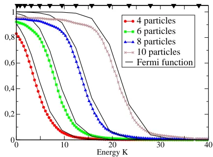
An inifite square well potential in one dimension has been investigated at a temperature of T = 2 K. The single-particle WF has been evaluated for N = 4,6,8 and 10 by means of equation (17). Then the average values of the points of the WF corresponding to energy intervalǫ,ǫ+δǫhave been plotted as a function ofǫ, in Fig. 2. Since the energy depends only upon the Wigner momentum of the particle (p2_{/2m), the above average} corresponds to the integral of the single-particle reduced WF with respect to the position variable (x). In our simulations the width of the well has been kept contant to a value of 150 nm.

A comparison between our curves and the Fermi func-tions is obtained by evaluating the chemical potentialsµ for N = 4,6,8 and 10 from a numerical solution of the equation:

N =

∞

X

n=1 1

eǫnkB T−µ _{+ 1}

. (19)

The curves in Fig. 2 show a very good agrement between the Fermi function and the average of the WF for any number of particles.

It is worth noting that, as expected, the agreement between the averages of WFs and the Fermi distributions is higher as the number of particles increases. However in Fig. 2 even in the case of 10 particles the value of the WF’s average corresponding to the point with ǫ= 0 do not reach the maximal value of 1. For this reason we have

0 10 20 30 40

Energy K 0

0,2 0,4 0,6 0,8 1

4 particles 6 particles 8 particles 10 particles Fermi function

FIG. 2: Average values of the points corresponding to the same energy inteval of the single-particle reduced WF of a system ofNparticles at thermal equilibrium at a temperature of 2 K in an 1D infinite square well potential. Since the energy depends only upon the momenta of the particles, the above average corresponds to the integral over the position variable (x). The width of the well has been fixed to 150 nm. In the upper part of the figure the black triangles indicate the energies corresponding to the eigenstates of the well.

0 2 4 6 8 10

Energy K 0,9

0,92 0,94 0,96 0,98 1

10 particles 26 particles 85 particles

FIG. 3: Average values of the points corresponding to the same energy of the single-particle reduced WF of a system of

Nparticles at thermal equilibrium at a temperature of 2 K in a 1D infinite square well potential. The width of the well has been fixed to 150 nm and the number of particles increased from 10 to 85.

0 5 10 15 20 Energy K

0 0,2 0,4 0,6 0,8 1

4 paricles 6 particles 8 particles 10 particles Fermi function

FIG. 4: Average values of the points corresponding to the same energy of the reduced single-particle WF in a harmonic potential with spring constantk= 1.54×108 [kg/sec2]. The

system in the case of N = 4,6,8,10 particles is studied at thermal equilibrium at a temperature of 2 K. The curves clearly tend to the Fermi-Dirac distribution. In the upper part of the figure the black triangles indicate the energies corresponding to the eigenstates of the harmonic potential.

B. Harmonic Potential

As a second example, we have studied a one-dimensional harmonic potential. Equation (17) has been evaluated for different numbers of particles (4,6,8 and 10) at a temperture of T = 2 K. The average over the points of the WF belonging to the same energy interval (p2_/2m+1

2kx2, wheremis the mass of any particle in the system) are plotted in Fig 4. The Fermi function with the chemical potential given by equation (19) is clearly approached by the corresponding average of the WF.

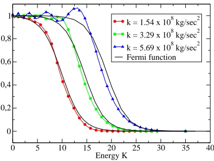
C. Effect of energy separation between levels

It is possible to study how the particle distributions change when the dimension of the well or the strength of the harmonic potential are varied in the case of both the infinite square well potential and the harmonic po-tential. When the width of the well decreases or the strength of the harmonic potential increases, the spacing between the allowed energy levels increases and an oscil-lating behaviour shows up in the curves (see Fig.s 5, 6). Our calculations have been performed in the case of a system with 10 particles at a temperature of 2 K. When the width of the well is decreased from 150 nm to 70 nm, the energy gap between the ninth and the tenth en-ergy level increases from 3.8 to 17.1 K. In the case of the harmonic potential the strength of the force constant is varied from 1.54×108_{to 5.69×10}8_kg/sec2_{leading to an} increase of the distance between the energy levels from 1

0 20 40 60 80 100 120 140 160 180 Energy K

0 0,2 0,4 0,6 0,8 1

L = 150 nm L = 110 nm L = 70 nm Fermi function

FIG. 5: Average values of the points corresponding to the same energy of the reduced single-particle WF in a 1D infi-nite square potential well. In a system with 10 particles at a temperature of 2 K, the width of the well has been reduced from 150 nm to 70 nm, that corresponds to an energy gap decrease, from the ninth to the tenth energy level, from 3.8 to 17.1 K. When the energy spacing between the levels is bigger than the thermal energy, the particles distribution deviates form a Fermi function.

to 2 K. The simulations show that such oscillations get more and more evident as the ratio between the spacing of the energy levels and kBT becomes greater. Under

these conditions the picture of a continuous spectrum of energies breaks down.

IV. TRANSPORT EQUATION

The dynamical equation for the single-particle WF is derived by differentiating the definition of the WF itself:

∂

∂tfW(r,p, t) = Z

dse−~isp∂ ∂t

h

ψr+s 2, t

ψ⋆_r

−₂s, ti.

(20) By means of the Schr¨odinger equation it is possible to evaluate the time derivative of the product of the two wave functions and to obtain the dynamical equation for the WF [4]:

∂

∂tfW(r,p, t) = − p

m∇fW(r,p, t) + 1

h3 Z

dp′_VW(r,p−p′)fW(r,p′, t),

(21)

whereVW is the interaction kernel for an external

poten-tialV(r). Note that the interaction term, given by:

VW(r,p)=

1 i~

Z dse−i

~ps h

Vr+s 2

−Vr₋s

2 i

0 5 10 15 20 25 30 35 40 Energy K

0 0,2 0,4 0,6 0,8 1

k = 1.54 x 108 kg/sec2

k = 3.29 x 108 kg/sec2

k = 5.69 x 108 kg/sec2 Fermi function

FIG. 6: Average values of the points corresponding to the same energy interval of the reduced single-particle WF in a harmonic potential. In the case of 10 particles the bound constant has been varied from k = 1.54×108 [kg/sec2] to k= 5.69×108 [kg/sec2] corresponding to an increase of the

spacing between the energy levels from 1 to 2 K. When the gap between the energy levels increases and becomes bigger than 2 K, the gas temperature, the particles distribution shows an oscillating behaviuor superimposed to the Fermi-like shape.

depends on the values of V at points different from r. However, while the non-locality ofVW extends to

infin-ity, its effect on the electron dynamics has to be consid-ered only up to regions where the electron correlation is different from zero.

A. Electron-Electron Scattering

Let us study the transport equation for electron-electron scattering. In the case where no phonons nor external forces are present, the potential V(r1,r2...rN)

is given by the Coulomb interaction, the transport equa-tion reads:

∂

∂tfW(r1,p1, ...,rN,pN, t) = − X

l

pl

m∇rlfW(r1,p1, ...,rl,pl, ...,rN,pN, t)

+1 ~3

X

i

X

j

Z

dp′_idp′_jδ(∆pi+ ∆pj)VW(|ri−rj|,∆pi−∆pj)

×fW(r1,p1, ...,ri,p′i, ...,rj,p′j, ...rN,pN, t),

(23)

whereVW is the potential kernel of the Wigner equation

and ∆p = p₋p′. As done before, in order to get a better understanding of the above equation, the kernel that describes the electron-electron interaction is studied forN = 2:

VW(r1,r2,p1,p2) = 1 i~

Z

ds1ds2e−

i

~(p1s1+p2s2)

×hVr1+

s1 2 ,r2+

s2 2

−Vr1−

s1 2 ,r2−

s2 2

i .

(24)

VW(r1,r2,p1,p2) = 1 i~

Z

dsds′e−i

~(p1+p2)s′_e−i

~(p1−p2)sh_Vx+ s

2

−Vx₋s

2 i

= ~ 3

i~δ(p1+p2)

Z dse−i

~(p1−p2)sh_Vx+s

2

−Vx₋s

2 i

= ~3_δ(p1+p2)VW(r1−r2,p1−p2). (25)

Thus the factor δ(∆pi+ ∆pj) appearing in equation

(23) represents the constrain for the total momentum consevation while the difference (∆pi−∆pj) indicates

that the interaction depends only upon the momentum transfer between particleiandj.

When the single-particle reduced WF in the case ofN particles is evaluated, equation (23) reads:

∂ ∂tf

(N)

W (r,p, t) = −

p m∇rf

(N)

W (r,p, t)

+1 ~3

Z

d̺ dp̺

Z

dp′VW(|r−̺|,2∆p)

×f_W(N)(r,p′, ̺,p̺, t), (26)

whererand pare the position and the Wigner momen-tum of the considered particle and, ̺ and p̺ indicate

the position coordinates of one of the remaining N −1

particles. It should be noticed that all the particles are interacting with each other, but, due to their indistin-guishability, all the contributions are identical and sum up to balance the factorials appearing in equation (2). The above expression shows that the transport equation for the reduced single-particle WF depends on the re-duced two-particle WF. When the transport equation for the reduced two-particle WF is evaluated, the electron-electron interaction term depends upon the three-particle reduced WF and so on for the transport equation for the other reduced WFs. It is the Wigner picture of the BBGKY hierarchy.

When the WF is written in terms of antisimmetric single-particle wave functions, as we have seen in equa-tion (5), two types of contribuequa-tions can be identified. It is then possible to study how the transport equation reads when only the contributions due to non overlapping wave functions are considered:

∂ ∂tf

(N)

W (r,p, t) =

∂ ∂t

X

i

fW(Ni)(r,p, t)

= −_mp∇rf

(N)

W (r,p, t) +

1 ~3

X

i

Z

dp′d̺ VW(|r−̺|,2∆p)



 X

j6=i

|ψj(̺)|2





×fWi(N)(r,p

′_{, t).}

(27)

Besides a Liouvillian contribution, an interaction term appears where each one-particle contribution interacts with all the others as in the Hartree approximation. In the case of overlapping wave functions also the other kind of contributions (as studied in equation (5)) must be con-sidered, and the exchange term is restored.

B. Electron-Phonon Scattering for the 2-Electrons WF

∂ ∂tfW

_ep

=X

q′

F(q′)

×nei(q′r1−ωq′(t−t0))p_n

q′ + 1fW

r1,p1− ~q′

2 ,r2,p2,{..., nq′+ 1, ...},{n

′ q}, t

−e−i(q′r1−ωq′(t−t0))√_n

q′f_W

r1,p1+ ~q′

2 ,r2,p2,{..., nq′−1, ...},{n

′ q}, t

+e−i(q′r1−ωq′(t−t0))

q n′

q′+ 1fW

r1,p1− ~q′

2 ,r2,p2,{nq},{..., n

′

q′+ 1, ...}, t

−ei(q′r1−ω_q′(t−t0))q_n′

q′fW

r1,p1+ ~q′

2 ,r2,p2,{nq},{..., n

′

q′−1, ...}, t

+o.p.

,

(28)

where r1,p1,r2,p2 are the Wigner phase space coordi-nates of the two particles. In the above equation o.p. stands for other particle and indicates the four terms wherer2replacesr1in the exponential factors andp2 un-dergoes a variation of~q′_{/2 whilep}

1remains unchanged. The eight terms appearing on the r.h.s. of the above equation have simple physical interpretations: the e-ph interaction occurs as emission or absorpion of a quantum of any modeq and this may appear in the state on the left or on the right of the bilinear expression that defines the WF. Each elementary interaction orvertexchanges only one of the two sets of variables of the WF; more precisely, one of the occupation numbers nq is changed

by unity and one of the electron momenta is changed by half of the phonon momentum.

In analogy with the Chambers formulation [16] of the classical kinetic equation it is possible to introduce new variables (r∗_i,p∗_i, t∗_{) that allow us to obtain an integral}

form of the dynamical equation for the WF. This inte-gral equation is in a closed form and can be solved by iteratively substituting it into itself, leading to what is known as its Neumann expansion.

Equation (28) gives 8 terms for the contribution of the first order of the Neumann expansion, 64 terms for the contribution of the second order and so on for the higher order terms. In order to obtain meaningful physi-cal quantities, however, the trace over the phonon modes must be performed, leading to a vanishing contribution for each term corresponding to an odd order in the Neu-mann expansion [8]. Only terms with an even number of verteces give dyagonal (in the phonon modes) contribu-tions different from zero.

As stated before, the second order in the Neumann expansion gives 64 terms. Among these, 32 yield con-tributions dyagonal in the phonon modes and survive to the trace operation, 16 terms refer to one particle and 16 to the other. For each particle 8 terms are the complex conjugate of the other 8 and can be summed together leading to 8 contributions for each particle. Among these it is possible to recognize four standard interactions

un-dergone by each particle: real emission; real absorption; virtual emission and virtual absorption.

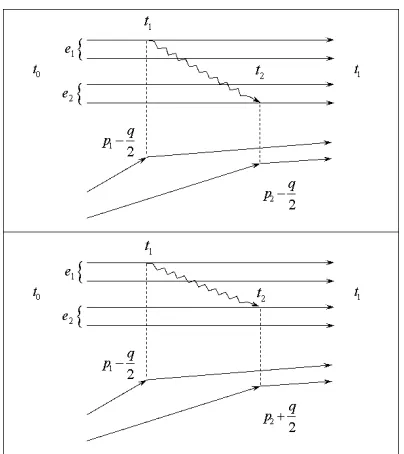
The main difference to the single particle case lies in the eight (four for each particle) remaining terms. In the two-particle case the phonon occupation number can be changed, in the first or second set of values in the arguments of the WF, not just by one electron loosing (gaining) a Wigner momentum equal to half the phonon momentum in each of the two verteces [8] but also by the action of two electrons. One electron looses or gains half phonon momentum in the first vertex and another elec-tron looses or gains half phonon momentum in the second vertex. Since we are dealing with identical particles we don’t know which electron interact with the phonon bath in the first or in the second vertex. These four terms are real or virtual emissions or absorptions where the inter-action with the phonon bath is shared between the two electrons.

It should be recalled that the p variable of the WF is obtained as a linear combination of two electron mo-menta. A specific value ˜pis obtained as ˜p=~₍k1+k2)/2 wherek1andk2 range from−∞to +∞. For this reason the Wigner momentum undergoes a change correspond-ing to half of the phonon momentum at each interaction vertex.

FIG. 7: Real emission of a phonon mode in mutual partecipa-tion by two electrons. One electrone1changes its Wigner

mo-mentum by half of the phonon momo-mentum at timet=t1and

the other electrone2does the same at a later timet=t2

(up-per bow). Virtual emission where one electron lose a Wigner momentum equal to half the momentum of the phonon while the other electron gains the same amount (lower bow).

In the lower box of Fig. 7 at time t =t2 an electron absorbs the phonon emitted att =t1, corresponding to a virtual emission.

V. CONCLUSION

We have developed a model based on the WF formal-ism that allows to introduce the symmetry effect in a sys-tem where electrons interact with each other and with the phonon bath. We have shown how this formalism can be usefull by applying it to different situations: the study of the electron-electron scattering, the study of the thermal distribution of N particles in confining potentials, and the study of the two-electron dynamics in the presence of electron-phonon scattering. We have also shown that with the WF it is possible to reproduce a Fermi like dis-tribution defining the energy in the Wigner phase-space.

Acknowledgments

This work has been partially supported by the U.S.Office of Naval Research (contract No. N00014-03-1-0289).

[1] E. Wigner, Phys. Rev., 40, 749-759, 1932 [2] W. Frensley, Rev Mod. Phys., 62, 745-791, 1990. [3] M. Nedjalkov et al., Phys. Rev. B, 70, 115319-115335,

2004.

[4] C. Jacoboni et al., Rep. Prog. Phys., 67, 1033-1071, 2004. [5] P. Carruters et al., Rew. Mod. Phys., 55, 245-285, 1983. [6] F. Rossi et al., Rev. Mod. Phys., 74, 895-950, 2002. [7] L.V. Keldysh, Zh. Eksp Teor. Fiz 47, 1515-1527, 1964,

Sov. Phys. JEPT 20, 1018, 1965.

[8] M. Pascoli et al., Phys. Rev. B., 58, 3503-3506, 1998.

[9] J.G. Kirkwood, Phys. Rev., 44, 31-37, 1933 [10] C. Harper, Am. J. Phys., 42, 396-399, 1974 [11] G.E. Uhlenbeck et al., Phys. Rev., 41, 79-89, 1932 [12] M. Hillery et al., Phys. Rep., 106, 121-167, 1984. [13] K. Imre et al., J. Math. Phys., 8, 1097-1108, 1967. [14] E. Cancellieri et al., J. Comp. Electron., 3, 411-415, 2004. [15] F. Reif, McGraw-Hill International Book Company,

“Sta-tistical and Thermal Physics”, 1965.